Robust bootstrap prediction intervals for univariate and multivariate autoregressive time series models
Abstract
The bootstrap procedure has emerged as a general framework to construct prediction intervals for future observations in autoregressive time series models. Such models with outlying data points are standard in real data applications, especially in the field of econometrics. These outlying data points tend to produce high forecast errors, which reduce the forecasting performances of the existing bootstrap prediction intervals calculated based on non-robust estimators. In the univariate and multivariate autoregressive time series, we propose a robust bootstrap algorithm for constructing prediction intervals and forecast regions. The proposed procedure is based on the weighted likelihood estimates and weighted residuals. Its finite sample properties are examined via a series of Monte Carlo studies and two empirical data examples.
Keywords: Autoregression; Multivariate forecast; Prediction interval; Resampling methods; Vector autoregression; Weighted likelihood.
1 Introduction
Forecasting future observations in autoregressive (AR) time series models is of great interest. Forecasts are usually obtained in the form of point and/or interval forecasts. A point forecast is an estimate of the unknown future observation conditional on the observed dataset. The point forecast provides a partial information since it does not provide any information about the degree of uncertainty associated with the forecasts. On the other hand, an interval forecast (or prediction interval) can provide reasonable inferences taking into account uncertainty associated with each point forecast (e.g., Chatfield, 1993; Kim, 2001; Jore et al., 2010). Classical techniques for calculating prediction intervals require strong assumptions, such as Gaussian forecast errors, known lag order, and model parameters. However, these assumptions are generally unknown in practice. They may also be affected by any departure from assumptions that leads to unreliable results. Alternative computational methods to construct prediction intervals without considering distributional assumptions include the use of well-known resampling-based procedures, such as the bootstrap.
Bootstrapping prediction intervals of the AR models have received much attention in the literature. Several bootstrap methodologies have been proposed to improve the empirical coverage accuracy of prediction intervals. Most relevant studies are based on the bootstrap procedure of Thombs and Schucany (1990). In the context of univariate AR models, Cao et al. (1997) proposed a computationally efficient bootstrap method. Masarotto (1990) and Grigoletto (1998) proposed alternative bootstrap techniques to obtain prediction intervals in the AR models when the true lag-order is unknown. Kabaila (1993) suggested bootstrap prediction intervals considering both unconditional inference and inference conditional on the last observed values. Breidt et al. (1995) introduced bootstrap prediction intervals for non-Gaussian autoregressions. Pascual et al. (2001) studied the effect of parameter estimation on prediction intervals. Clements and Taylor (2001) improved the empirical coverage accuracy of the bootstrap prediction intervals by applying parameter estimation bias-correction methods. Alonso et al. (2002) proposed the AR-sieve bootstrap procedure to construct nonparametric prediction intervals. Kim (2004) used asymptotically mean-unbiased parameter estimation to construct prediction intervals. Clements and Kim (2007) proposed to bootstrap prediction intervals for highly persistent AR time series; Mukhopadhyay and Samaranayake (2010) proposed a modified version of the AR-sieve bootstrap to obtain prediction intervals. Pan and Politis (2016) used forward and backward bootstrap methods with predictive and fitted residuals when constructing prediction intervals.
In the context of multivariate AR (VAR) models, bootstrap forecast densities/regions were constructed by Kim (1999), who extended the univariate bootstrap procedure of Thombs and Schucany (1990) to the VAR case. Kim (2001, 2004) proposed bias-corrected bootstrap forecast regions by using the bootstrap-after-bootstrap approach; and Fresoli et al. (2015) introduced a bootstrap method based on a forwarding representation for non-Gaussian unrestricted VAR models.
In the aforementioned literature, the bootstrap analog of AR forecasts is calculated using maximum likelihood, Yule-Walker, or ordinary least squares (OLS) estimators. It is well known that these estimators can be affected by the presence of the outliers, which is common in real datasets. In such cases, the estimates may be severely biased, and this can lead to poor finite sample properties of the bootstrap prediction intervals. On the other hand, robust estimation procedures can be irresponsive to outliers and produce consistent results. In the context of AR-type models, several robust estimation procedures have been proposed. For example, for univariate AR models, Denby and Martin (1979) proposed a class of generalized M-estimates to obtain robust estimates of the parameter of a first-order AR model. Collomb and Hardle (1986) proposed a nonparametric method to estimate the AR model and predict one-step-ahead observations. Connor et al. (1994) proposed a robust recurrent neural network-based learning algorithm to obtain robust predictions for time series. Sejling et al. (2009) proposed two recursive robust estimation algorithms for the estimation of AR models. Politis (2009) suggested an algorithm for the robust fitting of AR models. Maronna et al. (2006) discussed the effects of outliers on estimation methods in the AR models and proposed several robust procedures, including: 1) a robust Yule-Walker (Rob-YW) method that uses a robust estimation of the autocorrelation function with the Durbin-Levinson algorithm, 2) a robust regression (Rob-Reg) where the model parameters are estimated by the MM-type regression estimator proposed by Yohai (1987), 3) a robust filter algorithm (Rob-Flt) where the model parameters are computed by minimizing a robust scale of prediction residuals, and 4) a generalized M estimator based robust regression (Rob-GM). These methods are also discussed by Durre et al. (2015).
For the VAR models, Croux and Joossens (2008) suggested a robust estimation for the VAR models (Rob-VAR) using the multivariate least trimmed squares estimator of Agullo et al. (2008). Jonas (2009) proposed a robust procedure based on weighted least squares for estimating model parameters in the VAR models. Muler and Yohai (2013) introduced a new class of robust estimators for the VAR models by extending MM-estimators to the multivariate case.
The aforementioned methods produce robust parameter estimates and more reliable point forecasts in the presence of outliers compared with classical estimation methods. However, bootstrap prediction intervals based on these estimation methods may still not provide efficient inferences for future values, as they produce high forecasting errors corresponding to the outlying observations. Thus, an estimation method that is robust both in the estimation of model parameters and in producing forecasting errors is needed. We examine the impacts of outliers on bootstrapping prediction intervals in the univariate and multivariate AR models. Further, we propose a sufficiently robust bootstrap method for constructing prediction intervals. The proposed method is based on the minimum density power divergence estimator of Basu et al. (1998). Compared with classical techniques, this estimator produces more robust estimates in the presence of outliers or when model assumptions do not hold. Also, it provides weighted residuals used to calculate bootstrap pseudo datasets and forecasts. The residuals obtained by the minimum density power divergence estimator are adjusted by a weight function that down-weights the high errors corresponding to the outliers. In turn, the proposed bootstrap method provides more reliable prediction intervals than those obtained by classical and other robust methods.
In time series, several types of outliers, such as the additive outlier (AO), innovative outlier (IO), level shift outlier, and transitory change outlier have been proposed (see, e.g., Fox, 1972). In this study, we restrict our focus to AOs and IOs since they are the most troublesome and commonly studied outlier types in time series. Several Monte Carlo experiments under different data-generating and outlier-generating scenarios and empirical data examples are used to evaluate the finite sample properties of the proposed bootstrap prediction intervals. According to the numerical results in Section 3, the proposed robust procedure has competitive coverage performance with narrower interval length in comparison with the OLS and other robust estimation-based bootstrap prediction intervals. Our findings also show that the proposed method has a competitive performance compared with other methods when no contamination is present in the data.
The rest of the paper is organized as follows. In Section 2, we present detailed information about outlier types, the weighted likelihood estimation methodology, and bootstrap procedures and their proposed robust counterparts. Extensive Monte Carlo simulations are performed to examine the finite sample properties of the proposed method in Section 3. Empirical data examples are analyzed, and the results are presented in Section 4. Section 5 concludes the paper, along with some idea on how the methodology presented can be further extended.
2 Methodology
Forecasting future observations in the VAR models is similar to forecasting future observations in the univariate AR models. Thus, in this section, we discuss bootstrapping prediction intervals for the VAR models only. Bootstrapping prediction intervals of the AR models can be considered as a particular case of the VAR, where there is only a univariate observed time series. In Section 2.1, we first summarize the multivariate AO and IO types. Bootstrap prediction intervals of the VAR models and its robust counterparts are presented in Section 2.2.
2.1 Outliers
Let us consider an dimensional multivariate time series . It follows the VAR() model with the AR order if
| (2.1) |
where are the random vectors of the time series, is the vector of coefficients, which is a matrix containing the separate matrices column-wise as blocks, and is a normally distributed multivariate white noise with non-singular covariance matrix . Using the lag operator notation, model (2.1) is written as follows:
where is matrix a polynomial of order and is an dimensional constant vector.
Following Tsay et al. (2000), a multivariate time series with a multivariate outlier, , can be written as follows:
where denotes the size of the outlier and is the binary indicator variable that characterizes the outlier at time point . The outlier type (AO/IO) is defined based on the matrix polynomial . If an AO exists at time , then . On the other hand, if an IO is present at time , then .
An IO that affects innovation can be considered an extraordinary shock influencing the future values of the series . In contrast, an AO at time point affects only the corresponding data point , not future values of the series, and can have serious effects on the estimated model parameters, residuals, and accuracy of forecasts. Generally, an AO has a much greater effect on forecasting accuracy than an IO, because an IO at time affects only the corresponding residual . Still, an AO, which is far from the bulk of the data, causes a large residual and affects future residuals. For more information about the AOs, IOs, and their effects on the model parameters, consult Fox (1972), Chang et al. (1998) and McQuarrie and Tsai (2003) .
2.2 Bootstrapping prediction intervals
Let us consider the VAR() model given in (2.1). Let and for and be the fitted values of obtained by a suitable method such as OLS and -step-ahead unobservable future values, respectively. Then, the point forecast of is obtained as follows:
where is the estimated parameter matrix of and for . Define the forecast error covariance matrix by
where with and for (see, e.g., Lütkepohl, 1991, 2005). For the VAR models, the prediction interval for a given horizon is obtained in the form of an ellipsoid and/or Bonferroni cube (see, e.g., Lütkepohl, 1991; Kim, 1999). Under the assumption of Gaussian distributed errors, the prediction ellipsoid is obtained by the -step-ahead forecast density, which may be estimated as:
where is the estimated forecast error covariance matrix. The calculation of this prediction ellipsoid becomes complicated when the forecast horizon . Alternatively, a Bonferroni cube, which provides better forecast regions by taking into account the asymmetry of the distribution, is suggested by Lütkepohl (1991). Thus, we calculate only the Bonferroni cube in our numerical analyses.
As noted earlier, this procedure may not be sufficient to obtain accurate prediction intervals since it is based on the normality assumption, conformity to which is generally unknown in practice. Therefore, it may be affected by the departure from normality and lead to unreliable results. Alternatively, the bootstrap method may be used to construct a prediction interval for without considering any distributional assumption. The underlying idea behind this method is to approximate the distribution of future observations by drawing resamples conditional on the observed data. Early studies on the construction of bootstrap forecast regions in the VAR models were conducted by Kim (1999), who extended the idea of Thombs and Schucany (1990) to the VAR case. Kim (2001, 2004) proposed a bootstrap-after-bootstrap approach to obtain bias-corrected bootstrap forecast regions. Later, Fresoli et al. (2015) proposed a bootstrap procedure based on the forward recursion to decrease the complexity of the bootstrap method of Kim (1999). In this study, we consider the technique proposed by Fresoli et al. (2015) (abbreviated as “FRP” hereafter), whose algorithm is given below.
-
Step 1.
For a realization of -dimensional multivariate time series , determine the lag-order parameter by Akaike Information Criterion (AIC) and calculate the OLS estimator of the parameter matrix .
-
Step 2.
Compute the residuals , for . Let denote the empirical distribution function of the centered and re-scaled residuals, , where and is the calculated standard deviation of the residuals, respectively.
-
Step 3.
Generate the bootstrap observations via the following recursion:
where is an independent and identically distributed (iid) sample from and for .
-
Step 4.
Compute the OLS estimator for the bootstrap observations .
-
Step 5.
Conditional on the last original observations, obtain the -step-ahead bootstrap point forecast of , given by as follows:
where for and is randomly drawn from .
-
Step 6.
Steps 3-5 are repeated times to obtain bootstrap replicates for each .
Then, a Bonferroni cube is obtained as follows (see, e.g., Kim, 1999)
where , is the th quantile of the generated bootstrap distribution of the th element of , and denotes cartesian product.
2.2.1 Proposed bootstrap procedure
Let us consider the univariate AR() model and let be a set of realizations of a normally distributed white noise sequence. Then, the joint probability density of is defined as follows:
Now, let and , respectively, be a realization of a time series and residuals, where and are the vectors of initial values. Then, the conditional log-likelihood is obtained as follows:
The conditional maximum likelihood (CML) estimators of and are obtained by the solution of the score functions
It is well known that the CML method works well under the assumption of a correctly specified model and no outliers present in the data; however, when the data are contaminated by outliers, it produces biased estimates for the model parameters, and the errors computed corresponding to the outliers will be very large (see, e.g., McQuarrie and Tsai, 2003). Thus, the bootstrap prediction intervals based on CML may not provide reliable inferences in the presence of outliers.
Our proposal to construct a robust bootstrap prediction interval/forecast region for the AR models is to replace the CML (or OLS) estimators and residuals by weighted likelihood estimators and weighted residuals in the algorithm given in Section 2.2. The weighted likelihood methodology is suggested by Markatou (1996) and Markatou et al. (1998) to improve the robustness of the estimates, and has been studied in a wide variety of statistical applications; see, for example, Agostinelli and Markatou (2001), Agostinelli (2002a, b), and Agostinelli and Bisaglia (2010). It provides efficient estimators with high breakdown points when the errors are iid. Let and be a non-parametric kernel density estimator and smoothed model density (see, e.g., Markatou et al., 1998; Agostinelli and Bisaglia, 2010), respectively, defined as follows:
where , and , respectively, denote the empirical cumulative distribution function based on the residuals , the normal distribution function with zero mean and variance , and a kernel density with bandwidth . Note that both empirical cumulative distribution and normal distribution function are functions of . The Pearson residual , a measure of the discrepancy between and , and the weight function are defined as in (2.2) and (2.3), respectively:
| (2.2) | ||||
| (2.3) |
where is the positive part and denotes the residual adjustment function (RAF) of Lindsay (1994) (e.g., Hellinger RAF ). Then, the conditional weighted likelihood estimating equations for and are defined as in (2.4) and (2.5), respectively:
| (2.4) | |||
| (2.5) |
The weighted likelihood methodology defined above uses weighted score equations to estimate the model parameters. Considering the Pearson residuals in (2.2), if the model assumptions hold and no outliers are present in the data, then converges to 0, and so the weights converge to 1. In contrast, if the data are contaminated by outliers (i.e., if the observed frequency is relatively large compared with the predicted model ), the Pearson residuals will be large and the outlying observations will receive small weights. Since the weighted likelihood estimating equations given in (2.4) and (2.5) are defined on the weighted residuals, it will be robust against the outlying points.
As is mentioned above, the proposed robust bootstrap prediction interval/forecast region for the AR models is similar to the algorithm given in Section 2.2 except using weighted likelihood estimators and weighted residuals. Let , , and denote the weighted likelihood counterparts of , , and , respectively. Then, the weighted likelihood based -step-ahead bootstrap point forecast of , , is obtained by replacing with in the algorith given in Section 2.2.
Bootstrap prediction intervals based on the CML is very sensitive to outliers, and the estimated residuals corresponding to the outlying points will be large when it is used to estimate the AR model. Thus, the bootstrap prediction intervals based on the CML may not provide reliable results for the unobserved future sequence of the time series when the time series is contaminated by outliers. In contrast, bootstrap prediction intervals based on the weighted likelihood methodology are expected to have improved forecasting accuracy since it down-weights the high forecast errors produced by the outliers.
3 Numerical results
Under different scenarios and parameter settings, we conduct several Monte Carlo experiments to investigate the finite sample performance of our proposed weighted-likelihood based bootstrap prediction interval. For the univariate AR model, we compare our results with OLS-based bootstrap prediction intervals and four robust estimation-based bootstrap prediction intervals; Rob-YW, Rob-Reg, Rob-Flt, and Rob-GM. For the VAR model, the performance of the proposed bootstrap is compared with FRP and the multivariate least trimmed squares based bootstrap (Rob-VAR) method. For the univariate model, the comparison is made through the empirical coverage probability and length of bootstrap prediction intervals. The empirical coverage probability and volume of the bootstrap Bonferroni cubes, as well as the squared errors between the Bonferroni cubes obtained by the bootstrap methods and the empirical Bonferroni cube, are used as performance metrics for the VAR case.
Throughout the experiments, first, the synthetic datasets (or ) from the AR/VAR processes with sizes and , along with future values (or ), for each , are created. Then, bootstrap resamples are performed to obtain the bootstrap prediction intervals and Bonferroni forecast cubes. The coverage probabilities are calculated as the proportion of the generated future observations falling within the constructed bootstrap prediction intervals/Bonferroni forecast cube. For each model and sample size, this procedure is repeated for times to calculate the average values of the performance metrics. The significance level is set to 0.05 to obtain 95% bootstrap prediction intervals and/or Bonferroni cubes for future observations. The following method is used to calculate performance metrics.
-
Step 1.
Generate a univariate AR()/bivariate VAR() series, and for each , simulate future values based on the generated AR()/VAR() series.
-
Step 2.
Calculate bootstrap future values (or ) for and . Then, compute the average coverage probability of the bootstrap prediction interval for as:
Also, estimate the average coverage probabilities of bootstrap forecast regions for as:
-
Step 3.
Calculate the prediction interval length as:
and estimate the volume of the bootstrap Bonferroni cube using the following equation:
-
Step 4.
Calculate the squared error between the bootstrap and empirical Bonferroni cubes as follows:
Since our conclusions do not vary significantly with different sample sizes, to save space, we present only the results for ; the results obtained when can be obtained from the corresponding author on request.
3.1 Numerical results for the univariate AR model
For the univariate case, we consider the following AR(1) model:
| (3.6) |
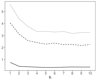
where . The modeling scenarios are adapted such that 1) no clear outlying data points are generated, 2) of only the generated training data are contaminated by deliberately inserted AOs or IOs, and 3) of the generated future values are contaminated by deliberately inserted AOs or IOs. AOs are generated by contaminating randomly selected observations with the value 5, while IOs are generated by contaminating randomly selected innovations with the value 3. For the first scenario, where no outlying observations are deliberately inserted into the dataset, we consider the parameter values and to assess the effect of parameter values on the bootstrap prediction intervals. For the second and third scenarios, the parameter values are fixed at and , and we check the effects of the number of outliers on the prediction intervals. For these cases, the average coverage probabilities when the bootstrap-based quantiles are replaced with the quantiles of the normal distribution are also calculated to explore whether bootstrapping improves the proposed and other statistical methods. The results are given in Figures 1-6.


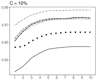


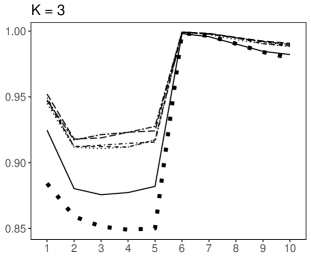


Our results show that when no fixed outlying data point is inserted into the dataset: 1) all the bootstrap prediction intervals tend to produce similar average coverage probabilities when the time series data are persistent (), with only the Rob-YW slightly differing from other methods; 2) the bootstrap procedure based on the weighted likelihood methodology generally produces improved coverage probabilities than other methods when the generated data are not persistent; 3) when the generated data are not persistent, the proposed method produces coverage probabilities close to the nominal level and generally results in slight under-coverage (over-coverage is observed only for the case when and , but is observed for all bootstrap prediction intervals based on different methods); and 4) the proposed bootstrap procedure has a smaller prediction interval length than other methods when the data are not persistent, while all bootstrap methods tend to produce similar interval lengths when . One exception is that Rob-Reg has smaller interval lengths than other methods when and . Note that, when the generated data have no deliberately inserted outliers, the proposed bootstrap method is expected to perform similarly to other methods. However, it performs better than other bootstrap prediction intervals in some cases, because some outlying observations with small magnitudes may be produced by the data generating process. The weighted likelihood method reduces the effects of such observations, giving the proposed method a slightly better performance than other methods in some cases.
When the training data have AOs, over-coverage (, in general) is observed for all bootstrap prediction intervals, excluding the proposed method because of the high forecasting errors produced in line with the outlying points. In contrast, the proposed procedure is less affected by these points and provides coverage probabilities close to the nominal level. In addition, the proposed idea has significantly narrower prediction intervals than other methods when AOs are present in the data (see Figure 3).
When the generated training data have IOs, compared with other methods, the proposed bootstrap method generally performs poorly for small in terms of empirical coverage probability. Under-coverage is observed for the proposed method while the other methods result in over-coverage. As in the AO case, the proposed bootstrap method produces significantly narrower prediction interval lengths compared with other methods. When comparing the performance of the bootstrap methods for the AO and IO cases (Figures 3 and 4), the results demonstrate that the bootstrap methods produce slightly lower coverage values when AOs are present in the generated datasets than those of IOs. This is due to fact that the bootstrap methods tend to produce wider prediction intervals when the data are contaminated by AOs compared to IO case. As is mentioned in Section 2.1, an AO at time influences corresponding residual as well as the future residuals (at time ) while an IO at time influences only the corresponding residual. Therefore, compared with the IO case, more high-valued forecast errors are present when the data have AOs. As a result, the bootstrap methods produces wider prediction intervals when AOs are present in the data compared with IOs, and thus, the prediction intervals cover more future values.
Moreover, our findings for the coverage probabilities indicate that bootstrap-based quantiles generally perform better than the quantiles of the normal distribution when the time series is generated without outliers. When the training data are contaminated by AOs, the proposed bootstrap method outperforms normal quantiles for small forecast horizons, while the quantiles obtained from the proposed method and the normal distribution produce similar coverage performances for mid-term and long-term forecast horizons. In contrast, when the training data are contaminated by IOs, the quantiles of the normal distribution perform better than all bootstrap-based quantiles for moderate and large values of , while the bootstrap-based quantiles perform better when is small. Our conclusions about the comparison between bootstrap-based and normal quantiles are restricted to data structures considered in this study, and may not be readily generalizable.
When the generated future values include AOs (see Figure 5), under-coverage is observed for all the bootstrap methods and normal quantiles. In this case, all the methods perform considerably less in terms of coverage probability compared with the second scenario, and their coverage performances get worse as the number of outliers increase. On the other hand, when the generated future observations have IOs (see Figure 6), for all bootstrap methods, under-coverage is observed for short-term forecast horizons while over-coverage is observed for long-term forecast horizons. For this scenario, the proposed bootstrap method produces smaller prediction interval length, among others.
3.2 Numerical results for the VAR model
The experimental design of our simulation study for the VAR case is somewhat similar to that of Fresoli et al. (2015). We consider the following VAR(2) model:
where
The distribution of the error process depends on the modeling scenarios; three error distributions-Gaussian , (heavy-tailed) and (skewed)-are considered when the data have no clear outliers while the errors are distributed as and when AOs or IOs are present in the data. To generate AOs, of the generated data are randomly selected, and both components contaminated by the value 5 while innovation terms are randomly selected and only the first component of the innovations are contaminated by the value 5 to generate the IOs.
Our results are reported in Figures 7-11. When no outlier is present in the data, all bootstrap methods tend to produce similar coverage probabilities and volume of forecast cubes, as shown by Figure 7. Only the Rob-VAR produces slightly different coverage probabilities compared with the proposed and OLS methods when the errors follow and distributions. Figure 7 also shows that the proposed method has fewer errors than the other two methods when the errors are generated from and distributions. However, it produces larger errors than the other methods when the errors follow a distribution.


When the data have AOs/IOs and the error terms follow distribution, the proposed method has significantly better performance compared with the other two methods. In other words, the proposed method produces better coverage probabilities, less volume, and Bonferroni forecast cubes more similar to the empirical Bonferroni forecast cube compared with other bootstrap methods. All the methods result in under-coverage when outliers contaminate the data; however, the coverage probabilities produced by the proposed method are much closer to the nominal level than those of other bootstrap methods (see Figures 8 and 9). When the data have AOs/IOs but distributed error terms (Figures 10 and 11), the proposed method still has a superior performance over other methods, but it performs slightly worse compared with the case where the errors follow distribution.
4 Empirical data examples
Through two data analyses, we study the forecasting performance of the proposed method. For the univariate AR model, we consider monthly Brazil/U.S. dollar exchange rate data; quarterly GDP and immediate rate (IR) data for Turkey are considered for the VAR model. Both sets of data can be found at https://stlouisfed.org.
4.1 Brazil/U.S. dollar exchange rate data
Original monthly Brazil/U.S. dollar exchange rate data were obtained starting from February 1, 1999 to August 1, 2018 (235 observations), and a logarithmic return series generated via
where represents the observed exchange rate at the th month. Time series plots of the original and logarithmically transformed exchange rate data are presented in Appendix, which shows several clear outlying observations.
The -values obtained by the Ljung-Box (LB) and augmented Dickey-Fuller (ADF) -statistics tests (-value ) suggest that the return series is a stationary process with mean zero. The autocorrelation and partial-autocorrelation plots of the return series (not presented here) show that an AR model may be appropriate to model the return series. The optimal lag order for this series is obtained as 3, AR(3), via the AIC. In addition, the structural break test based on statistics in the R package strucchange of Zeileis et al. (2002) is applied to the returns series to check if there is a structural break in the series. In this test, a statistic is computed for every predetermined potential change point and the structural break test is performed using the calculated statistics. For the return series of monthly Brazil/U.S. dollar exchange rate data, this test procedure produce the -value, which indicates that there is no clear structural break in the data.
To obtain out-of-sample bootstrap prediction intervals for the return series, we divide the data into two parts; we estimate the model based on observations from February 1, 1999, to August 1, 2017, to construct -step-ahead prediction intervals from September 1, 2017, to August 1, 2018. Our results are shown in Figure 12, which shows the prediction interval produced by the proposed method is narrower than those obtained by other bootstrap methods, and all prediction intervals include all the observed future values.

4.2 Real GDP and immediate rate data for Turkey
Quarterly GDP and IR data for Turkey, which consist of 76 observations, were obtained for 1999 to 2017. The GDP and IR data were then logarithmically transformed as and , respectively. The time series plots of the original and transformed data are given in Appendix, which shows several outliers for both series.
For this dataset, the model is constructed based on data spanning from 1999 to 2016 to calculate Bonferroni cubes for four-step-ahead forecasts from 2016 to 2017. Table 1 presents the sample statistics and Jarque-Bera (JB) normality and ADF stationarity test results. The results indicate that: 1) the data do not follow a Gaussian process, either individually or jointly, and 2) both GDP and IR series are stationary processes according to ADF test results. Moreover, the results of the LB test (not presented here) indicate that there is a dynamic dependence on the conditional mean for this dataset. The optimal lag-order is determined by AIC, with the results showing that a VAR(3) model is optimal.
| Series | Mean | Sd | Skewness | Kurtosis | JB | ADF |
|---|---|---|---|---|---|---|
| 1.22 | 2.37 | 2.22 | 0.73 | 14.85 | -4.27 | |
| (0.00) | () | |||||
| -3.32 | 32.51 | 3.87 | 9.84 | 382.83 | -4.33 | |
| (0.00) | () | |||||
| () | 1.76 | 18.78 | 179.54 | |||
| (0.00) |

The constructed Bonferroni forecast cubes and observed out-of-sample values are presented in Figure 13. The bootstrap forecast cubes have considerably less volume than the Bonferroni cubes obtained by other bootstrap methods that use the OLS and multivariate least trimmed squares. Because of the high forecast errors caused by the presence of outliers, the weighted likelihood-based bootstrap method is less affected by the outliers and it thus provides Bonferroni cubes with less volume than the other two bootstrap methods.
5 Conclusion
We propose a robust procedure to obtain prediction intervals and multivariate forecast regions for future values in the AR and VAR models. The proposed idea is based on using the weighted likelihood estimators and weighted residuals, which are calculated under the assumption of normally distributed error terms, in the bootstrap method. The finite sample properties of the proposed method are examined via several Monte Carlo studies and two empirical data examples, and results are compared with classical and other existing robust methods. Our records show that the proposed procedure has similar coverage performance with generally smaller interval length/volume of forecast cube compared with existing bootstrap methods, when the data have no outliers. In addition, it has superior performance in terms of coverage and interval length/volume than the other bootstrap methods, when outliers are present in the data and the error terms follow a normal distribution.
The proposed method may lose some efficiency in its coverage performance when the errors differ from normality (such as when the errors follow distribution). This is because the weights do not converge to 1, when the errors follow a non-normal distribution. However, our results have demonstrated that the proposed method is also flexible enough to treat deviances from the normality and produces superior performance over the existing methods. For future research, the proposed method could be used to construct prediction intervals for financial returns and volatilities, in autoregressive conditional heteroskedasticity models (see, e.g., Pascual et al., 2006; Chen et al., 2011; Beyaztas and Beyaztas, 2018, 2019; Beyaztas et al., 2018).
Appendix: Additional figures for the empirical data analyses


References
- (1)
- Agostinelli (1998) Agostinelli, C. (1998), Inferenza Statistica Robusta Basata Sulla Funzione di Verosimiglianza Pesata: Alcuni Sviluppi, Phd thesis, University of Padova.
- Agostinelli (2002a) Agostinelli, C. (2002a), ‘Robust model selection in regression via weighted likelihood methodology’, Statistics & Probability Letters 56(3), 289–300.
- Agostinelli (2002b) Agostinelli, C. (2002b), ‘Robust stepwise regression’, Journal of Applied Statistics 29(6), 825–840.
- Agostinelli and Bisaglia (2010) Agostinelli, C. and Bisaglia, L. (2010), ‘ARFIMA processes and outliers: A weighted likelihood approach’, Journal of Applied Statistics 37(9), 1569–1584.
- Agostinelli and Markatou (2001) Agostinelli, C. and Markatou, M. (2001), ‘Test of hypotheses based on the weighted likelihood methodology’, Statistica Sinica 11(2), 499–514.
- Agullo et al. (2008) Agullo, J., Croux, C. and Aelst, S. V. (2008), ‘The multivariate least-trimmed squares estimator’, Journal of Multivariate Analysis 99(3), 311–338.
- Alonso et al. (2002) Alonso, A. M., Pena, D. and Romo, J. (2002), ‘Forecasting time series with sieve bootstrap’, Journal of Statistical Planning and Inference 100(1), 1–11.
- Basu et al. (1998) Basu, A., Harris, I. R., Hjort, N. L. and Jones, M. C. (1998), ‘Robust and efficient estimation by minimising a density power divergence’, Biometrika 85(3), 549–559.
- Beyaztas and Beyaztas (2018) Beyaztas, B. H. and Beyaztas, U. (2018), ‘Block bootstap prediction intervals for GARCH processes’, REVSTAT-Statistical Journal in press.
- Beyaztas et al. (2018) Beyaztas, B. H., Beyaztas, U., Bandyopadhyay, S. and Huang, W. M. (2018), ‘New and fast block bootstrap-based prediction intervals for GARCH(1,1) process with application to exchange rates’, Sankhya, Series A 80(1), 168–194.
- Beyaztas and Beyaztas (2019) Beyaztas, U. and Beyaztas, B. H. (2019), ‘On jackknife-after-bootstrap method for dependent data’, Computational Economics 53(4), 1613–1632.
- Breidt et al. (1995) Breidt, F. J., Davis, R. A. and Dunsmuir, W. T. M. (1995), ‘Improved bootstrap prediction intervals for autoregressions’, Journal of Time Series Analysis 16(2), 177–200.
- Cao et al. (1997) Cao, R., Febrerobande, M., Gonzalez-Manteiga, W., Prada-Sanchez, J. M. and Garcfa-Jurado, I. (1997), ‘Saving computer time in constructing consistent bootstrap prediction intervals for autoregressive processes’, Communications in Statistics - Simulation and Computation 26(3), 961–978.
- Chang et al. (1998) Chang, I., Tiao, G. C. and Chen, C. (1988), ‘Estimation of time series parameters in the presence of outliers’, Technometrics 30(2), 193–204.
- Chatfield (1993) Chatfield, C. (1993), ‘Calculating interval forecasts’, Journal of Business and Economics Statistics 11(2), 121–135.
- Chen et al. (2011) Chen, B., Gel, Y. R., Balakrishna, N. and Abraham, B. (2011), ‘Computationally efficient bootstrap prediction intervals for returns and volatilities in ARCH and GARCH processes’, Journal of Forecasting 30(1), 51–71.
- Clements and Kim (2007) Clements, M. P. and Kim, J. (2007), ‘Bootstrap prediction intervals for autoregressive time series’, Computational Statistics & Data Analysis 51(7), 3580–3594.
- Clements and Taylor (2001) Clements, M. P. and Taylor, N. (2001), ‘Bootstrapping prediction intervals for autoregressive model’, International Journal of Forecasting 17(2), 247–267.
- Collomb and Hardle (1986) Collomb, G. and Hardle, W. (1986), ‘Strong uniform convergence rates in robust nonparametric time series analysis and prediction: Kernel regression estimation from dependen observations’, Stochastic Processes and their Applications 23(1), 77–89.
- Connor et al. (1994) Connor, J. T., Martin, R. D. and Atlas, L. E. (1994), ‘Recurrent neural networks and robust time series prediction’, IEEE Transactions on Neural Networks 5(2), 240–254.
- Croux and Joossens (2008) Croux, C. and Joossens, K. (2008), Robust estimation of the vector autoregressive model by a least trimmed squares procedure, in P. Brito, ed., ‘COMPSTAT 2008’, Springer, Physica-Verlag.
- Denby and Martin (1979) Denby, L. and Martin, R. D. (1979), ‘Robust estimation of the first-order autoregressive parameter’, Journal of the American statistical Association: Theory and Methods 74(365), 140–146.
- Durre et al. (2015) Durre, A., Fried, R. and Liboschik, T. (2015), ‘Robust estimation of (partial) autocorrelation’, WIREs Computational Statistics 7(3), 205–222.
- Fox (1972) Fox, A. J. (1972), ‘Outliers in time series’, Journal of the Royal Statistical Society, Series B 34(3), 350–363.
- Freedman (1984) Freedman, D. (1984), ‘On bootstrapping two-stage least-squares estimates in stationary linear models’, The Annals of Statistics 12(3), 827–842.
- Fresoli et al. (2015) Fresoli, D., Ruiz, E. and Pascual, L. (2015), ‘Bootstrap multi-step forecasts of non-Gaussian VAR models’, International Journal of Forecasting 31(3), 834–848.
- Grigoletto (1998) Grigoletto, M. (1998), ‘Bootstrap prediction intervals for autoregressions: Some alternatives’, International Journal of Forecasting 14(4), 447–456.
-
Jonas (2009)
Jonas, P. (2009), Robust estimation of the
VAR model, in ‘Proceedings of the 18th Annual Conference of Doctoral
Students - WDS 2009’, MATFYZPRESS, Prague.
http://citeseerx.ist.psu.edu/viewdoc/download?doi=10.1.1.186.8431&rep=rep1&type=pdf - Jore et al. (2010) Jore, A. S., Mitchell, J. and Vahey, S. P. (2010), ‘Combining forecast densities from VARs with uncertain instabilities’, Journal of Applied Econometrics 25(4), 621–634.
- Kabaila (1993) Kabaila, P. (1993), ‘On bootstrap predictive inference for autoregressive processes’, Journal of Time Series Analysis 14(5), 473–484.
- Kim (1999) Kim, J. H. (1999), ‘Asymptotic and bootstrap prediction regions for vector autoregression’, International Journal of Forecasting 15(4), 393–403.
- Kim (2001) Kim, J. H. (2001), ‘Bootstrap after bootstrap prediction intervals for autoregressive models’, Journal of Business and Economic Statistics 19(1), 117–128.
- Kim (2004) Kim, J. H. (2004), ‘Bias-corrected bootstrap prediction regions for vector autoregression’, Journal of Forecasting 23(2), 141–154.
- Lindsay (1994) Lindsay, B. G. (1994), ‘Efficiency versus robustness: the case for minimum Hellinger distance and related methods’, The Annals of Statistics 22(2), 1018–1114.
- Lütkepohl (1991) Lütkepohl, H. (1991), Introduction to Multiple Time Series Analysis, 2nd edn, Springer-Verlag, Berlin.
- Lütkepohl (2005) Lütkepohl, H. (2005), New Introduction to Multiple Time Series Analysis, Springer-Verlag, Berlin.
- Markatou (1996) Markatou, M. (1996), ‘Robust statistical inference: Weighted likelihoods or usual M-estimation?’, Communications in Statistics - Theory and Methods 25(11), 2597–2613.
- Markatou et al. (1998) Markatou, M., Basu, A. and Lindsay, B. G. (1998), ‘Weighted likelihood estimating equations with a bootstrap root search’, Journal of the American Statistical Association: Theory and Methods 93(442), 740–750.
- Maronna et al. (2006) Maronna, R. A., Martin, R. D. and Yohai, V. J. (2006), Robust Statistics: Theory and Methods, Wiley, Chichester.
- Masarotto (1990) Masarotto, G. (1990), ‘Bootstrap prediction intervals for autoregressions’, International Journal of Forecasting 6(2), 229–239.
- McQuarrie and Tsai (2003) McQuarrie, A. D. and Tsai, C. (2003), ‘Outlier detections in autoregressive models’, Journal of Computational and Graphical Statistics 12(2), 450–471.
- Mukhopadhyay and Samaranayake (2010) Mukhopadhyay, P. and Samaranayake, V. A. (2010), ‘Prediction intervals for time series: A modified sieve bootstrap approach’, Communications in Statistics - Simulation and Computation 39(3), 517–538.
- Muler and Yohai (2013) Muler, N. and Yohai, V. J. (2013), ‘Robust estimation for vector autoregressive models’, Computational Statistics & Data Analysis 65, 68–79.
- Pan and Politis (2016) Pan, L. and Politis, D. N. (2016), ‘Bootstrap prediction intervals for linear, nonlinear and nonparametric autoregressions’, Journal of Statistical Planning and Inference 177, 1–27.
- Pascual et al. (2001) Pascual, L., Romo, J. and Ruiz, E. (2001), ‘Effects of parameter estimation on prediction densities: A bootstrap approach’, International Journal of Forecasting 17(1), 83–103.
- Pascual et al. (2006) Pascual, L., Romo, J. and Ruiz, E. (2006), ‘Bootstrap prediction for returns and volatilities in GARCH models’, Computational Statistics & Data Analysis 50(9), 2293–2312.
- Politis (2009) Politis, D. N. (2009), ‘An algorithm for robust fitting of autoregressive models’, Economics Letters 102(2), 128–131.
- Sejling et al. (2009) Sejling, K., Madsen, H., Holst, J., Holst, U. and Englund, J.-E. (1994), ‘Methods for recursive robust estimation of AR parameters’, Computational Statistics & Data Analysis 17(5), 509–536.
- Thombs and Schucany (1990) Thombs, L. A. and Schucany, W. R. (1990), ‘Bootstrap prediction intervals for autoregression’, Journal of the American Statistical Association: Theory and Methods 85(410), 486–492.
- Yohai (1987) Yohai, V. J. (1987), ‘High breakdown-point and high efficiency estimates for regression’, The Annals of Statistics 15(2), 642–656.
- Zeileis et al. (2002) Zeilesi, A., Leisch, F., Hornik, K. and Kleiber, C. (2002), ‘An R package for testing for structural change in linear regression models’, Journal of Statistical Software 7(2), 1–38.
- Tsay et al. (2000) Tsay, R. S., Pena, D. and Pankratz, A. E. (2000), ‘Outliers in multivariate time series,’, Biometrika 87(4), 789–804.