Robust Beamforming Design for Covert Communications
Abstract
In this paper, we consider a common unicast beamforming network where Alice utilizes the communication to Carol as a cover and covertly transmits a message to Bob without being recognized by Willie. We investigate the beamformer design of Alice to maximize the covert rate to Bob when Alice has either perfect or imperfect knowledge about Willie’s channel state information (WCSI). For the perfect WCSI case, the problem is formulated under the perfect covert constraint, and we develop a covert beamformer by applying semidefinite relaxation and the bisection method. Then, to reduce the computational complexity, we further propose a zero-forcing beamformer design with a single iteration processing. For the case of the imperfect WCSI, the robust beamformer is developed based on a relaxation and restriction approach by utilizing the property of Kullback-Leibler divergence. Furthermore, we derive the optimal decision threshold of Willie, and analyze the false alarm and the missed detection probabilities in this case. Finally, the performance of the proposed beamformer designs is evaluated through numerical experiments.
Index Terms:
Covert communications, covert beamformer design, zero-forcing beamformer design, robust beamformer design.I Introduction
Due to its broadcasting nature, wireless communication is vulnerable to malicious attackers. By exploiting encryption and key exchange techniques, conventional security methods mainly focus on preventing the transmitted wireless signals form being decoded by unintended users [1, 2], but not concealing them. For many wireless scenarios, such as law enforcement and military communications, the transmitted signals should not be detected in order to perform the undercover missions. Therefore, the paradigm of covert communications, also known as low probability of detection (LPD) communications, aims to hide the transmissions status, and protect the users’ privacy.
In a typical covert communication scenario, the sender (Alice) wants to send the information to the covert receiver (Bob) without being detected by the eavesdropper (Willie). Here, Willie may or may not be a legitimate receiver, while its purpose is to detect whether the transmission from Alice to Bob happens based on its observations. Mathematically, the ultimate goal for Willie is to distinguish the two hypothesis or by applying a specific decision rule, where denotes the null hypothesis that Alice does not transmit a private data stream to Bob, and denotes the alternate hypothesis that Alice transmits a private data stream to Bob [3]. In general, the priori probabilities of hypotheses and are assumed to be equal, i.e., each equal to . As such, the detection error probability of Willie is defined as in [3, 4, 5]
| (1) |
where indicates that Alice sends information to Bob, and indicates the other case. Covert communication is achieved for a given if the detection error probability is no less than , i.e., . Here, is a predetermined value to specify the covert communication constraint.
Although practical covert communications has been studied by investigating spread-spectrum technology [6] for several decades, the information-theoretic limits of covert communication were only recently derived [5, 7, 8]. The achievability of the square root law (SRL) was established in [5] where in order to achieve covert communication over the additive white Gaussian noise (AWGN) channel, Alice can only transmit no more than bits to Bob in channel uses. Moreover, the SRL results have been verified in discrete memoryless channels (DMCs) [8, 7], two-hop systems[9], multiple access channels [10] and broadcast channels [11]. In short, these results imply that the average number of covert bits per channel use asymptotically approaches zero despite the noiseless transmission, i.e., .
Fortunately, some works have revealed that Alice can achieve a positive covert rate under some given conditions, i.e., imperfect knowledge of noise [12, 13, 14]; imperfect channel statistics [15, 16]; unknown transmission time [17, 18, 19]; the presence of random jamming signals [20, 21]; finite blocklengths of transmissions [22, 23]; the existence of relay [24, 25, 26]; and appearance of injecting artificial noise (AN) [27, 28]. To be more specific, in [25], the authors proposed a power allocation strategy to maximize the secrecy rate under the covert requirements with multiple untrusted relays. Based on the proposed rate-control and power-control strategies, the authors in [24] verified the feasibility of covert transmission in amplify and forward one-way relay networks. With a finite number of channel uses, delay-intolerant covert communications was investigated in [22], which demonstrated that random transmit power can enhance covert communications. In addition, the effect of the finite blocklength (i.e., finite ) on covert communication was investigated in [28]. By exploiting a full-duplex (FD) receiver, covert communications was examined in [28] under fading channels, where the FD receiver generates artificial noise to confuse Willie. In [4], the optimality of Gaussian signalling was investigated by employing Kullback-Leibler (KL) divergence as a covert metric. By formulating LPD communications as a quickest detection problem, the authors in [23] investigated covert throughput maximization problems with three different detection methods, i.e., the Shewhart, the cumulative sum (CUSUM), and the Shiryaev-Roberts (SR) tests. With the help of a friendly uninformed jammer, Alice can also communicate covert bits to Bob in channel uses [20, 21]. By producing artificial noise to inhibit Willie’s detection, Alice can reliably and covertly transmit information to Bob [27].
Most existing works [5, 7, 8, 9, 10, 11, 20, 21, 24, 27, 22, 28, 4, 23, 29, 30] investigate covert transmission with perfect channel state information (CSI) of all users. However, covert communication for multiple antenna beamforming [31] has rarely been studied to the best of our knowledge, and in practical scenarios the perfect CSI of warden is usually not available. In [31], the authors investigated power allocation to maximize the secrecy rate while satisfying the covert communication requirements. In [32], the three-dimensional (3D) beamformer and jamming interference beamformer were iteratively optimized for maximizing the covert rate. In this work, we show that using multiple antennas allows us to relax the perfect CSI assumption while still guarantees convert transmission.
In this paper, we consider a practical scenario where Alice uses the communication link with Carol as a cover, and aims to achieve covert communication with Bob against Willie. The most relevant work to this paper is [16]. In [16], a single-input-single-output (SISO) covert communication scenario was considered, and an exact expression for the optimal threshold of Warden’s detector was derived. The authors then analyzed the achievable rates with outage constraints under imperfect CSI. However, in our work, we focus on a multiple-input-single-output (MISO) covert network for both the perfect CSI and imperfect CSI cases.
Our main contributions are summarized as follows:
-
•
When Willie’s CSI (WCSI) is perfect at Alice, we study the joint beamformer design problem with the objective of maximizing the achievable rate of Bob, subject to the perfect covert transmission constraint, quality of service (QoS) of Carol, and the total transmit power constraints of Alice. The covert rate maximization problem is shown to be non-convex. Then, by applying the semidefinite relaxation (SDR) technique and the bisection method, we find the solution by solving a series of convex subproblems.
-
•
Furthermore, to reduce the computational complexity, we propose a low-complexity zero-forcing (ZF) beamformer design with a single iteration processing, which provides a promising tradeoff between complexity and performance. Such design problem is transformed into two decoupled subproblems. To be specific, the design of Willie’s ZF beamformer can be relaxed to a convex problem by SDR, and Bob’s ZF beamformer design can be reformulated as a convex second-order cone program (SOCP) problem.
-
•
When WCSI is imperfect at Alice, we consider the robust covert rate maximization problem under the QoS constraint of Carol, the covertness constraint, and the total power constraint. To handle this non-convex problem, a restriction and relaxation method is introduced, and a convex convex semidefinite program (SDP) is obtained by using the S-lemma and SDR. Given that the covert constraint is not perfect, we derive the optimal detection threshold of Willie, and the corresponding detection error probability based on the robust beamformer vector. Such result can be used as the theoretical benchmark to evaluate the covert performance of beamformers deign. Our simulation results further reveal the tradeoff between Willie’s detection performance and Bob’s covert rate.
The rest of this paper is organized as follows. In Section II, we introduce the system model, assumptions and the notations used throughout the paper. In Section III, we discuss the covert beamformer and the ZF beamformer designs with perfect WCSI. In Section IV, we consider a robust beamforming design with imperfect WCSI. In Section V, we present numerical results to evaluate the proposed beamformers, and finally the paper is concluded in Section VI.
Notations: Boldfaced lowercase and uppercase letters represent vectors and matrices, respectively. and denote the real part and imaginary part of its argument, respectively. A complex-valued circularly symmetric Gaussian distribution with mean and variance is denoted by .
II System Model
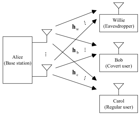
We consider the scenario illustrated in Fig. 1, in which Alice (base station) transmits data stream to Carol (regular user) all the time, and transmits private data stream to Bob (covert user) occasionally. For simplicity, let , . At the same time, Willie (eavesdropper) silently (passively) observes the communication environment and tries to identify whether Alice is transmitting to Bob or not. As we mentioned in the previous section, Alice may achieve covert communication by using the transmission to Carol as a cover. Suppose that Alice is equipped with antennas, while Carol, Bob and Willie each has a single antenna111 Under this setup, Willie only needs to perform energy detection and does not have to know the beamforming vectors.. Let , and denote the channel vectors from Alice to Bob, Carol and Willie, respectively. We assume that all channels are modeled as Rayleigh flat fading, i.e., , , and [16], where , and denote the variances of channels , and , respectively.
Recall that the goal for Willie is to determine which hypothesis ( or ) is true by applying a specific decision rule. For convenience, we use () to indicate the event that Alice does (does not) send information to Bob.
II-A Signal Model and Covert Constraints
From Willie’s perspective, Alice’s transmitted signal is given by
| (4) |
where and denote the transmit beamformer vectors for in hypothesis and hypothesis , respectively; denotes the transmit beamformer vector for . Let denote the maximum transmit power of Alice. Therefore, the beamformer vectors satisfy: under and under .
For Carol, the received signal is given by
| (7) |
where is the received noise at Carol222 Here, the inter cell interference is modeled as white Gaussian noise..
For Bob, the received signal is given by
| (10) |
where is the received noise at Bob.
In addition, the signals received by Willie can be written as
| (13) |
where is the received noise at Willie.
According to (7), we assume that the instantaneous rates at Carol are expressed as and under and , respectively, and can be written as
| (14a) | |||
| (14b) | |||
Similarly, based on (10), we assume that is the instantaneous rate at Bob under hypothesis , which is given by
| (15) |
Since Willie needs to distinguish between the two hypotheses from its received signal , we further characterize the probability of . Let and denote the likelihood functions of the received signals of Willie under and , respectively. Based on (13), and are given as
| (16a) | |||
| (16b) | |||
where and .
Recall from the previous section that Willie wants to minimize the detection error probability (1) by applying an optimal detector. To take into our problem formulation, we next specify conditions on the likelihood functions such that covert communication can be achieved with the given . First, we let
| (17) |
where is the total variation between and . In general, computing analytically is intractable. Thus, we adopt Pinsker’s inequality [33], and can obtain
| (18a) | |||
| (18b) | |||
where denotes the KL divergence from to , and is the KL divergence from to . Furthermore, and are respectively given as
| (19a) | ||||
| (19b) | ||||
Therefore, to achieve covert communication with the given , i.e., , the KL divergences of the likelihood functions should satisfy one of the following constraints:
| (20a) | |||
| (20b) | |||
II-B CSI Availability
In this subsection, we assume that Alice can accurately estimate the CSI of Bob and Carol. In most cases, such CSI can be learned at both the receiver side and the transmitter side by training and feedback. However, the WCSI may not be always accessible to Alice because of the potential limited cooperation between Alice and Willie. As a result, we consider the following two scenarios333 When Willie is totally passive, the covert communications scheme design may turn to exploit the channel distribution information of Willie [34, 31, 32, 35] :
1) Scenario 1. Perfect WCSI: We first consider a scenario that often arises in practice, where Willie is a legitimate user and is only hostile to Bob. In this case, Alice knows the full CSI of the channel , and uses it to help Bob to hide from Willie [5, 22, 28].
2) Scenario 2. Imperfect WCSI: We consider a more practical scenario where Willie is a regular user with only limited cooperation to Alice. In this case, Alice has imperfect CSI knowledge due to the passive warden and channel estimation errors [16, 36]. Here, the imperfect WCSI is modeled as
| (21) |
where denotes the estimated CSI vector between Alice and Willie, and denotes corresponding CSI error vector. Moreover, the CSI error vector is characterized by an ellipsoidal region, i.e.,
| (22) |
where controls the axes of the ellipsoid, and determines the volume of the ellipsoid [37, 32].
III Proposed Covert Transmission for Perfect WCSI
In this section, we consider the perfect WCSI scenario (scenario 1) and maximize the covert rate to Bob by optimizing beamformers at Alice. Specifically, we study a joint beamforming design problem with the objective of maximizing the achievable rate of Bob , subject to the perfect covert transmission constraint, QoS of Carol, and the total transmit power constraints of Alice, which can be mathematically formulated as
| (23a) | ||||
| s.t. | (23b) | |||
| (23c) | ||||
| (23d) | ||||
Note that, is a function of , and is a function of both and for (23c). Thus, and can be expressed as and , respectively.
Notice that problem (23) is non-convex and difficult to be optimally solved. Moreover, constraints and are equivalent for the perfect covert transmission case.
To address the non-convex problem (23), we propose two beamformers design approaches, namely, the proposed covert beamformer design and proposed ZF beamformers design.
III-A Proposed Covert Beamformer Design
To simplify the derivation, define and , and introduce an auxiliary variable . Then, problem (23) can be reformulated as the following equivalent form:
| (24a) | ||||
| (24b) | ||||
| (24c) | ||||
| (24d) | ||||
| (24e) | ||||
Next, we apply the SDR technique [38] to relax problem (24). Towards this end, by using the following conditions
| (25a) | |||
| (25b) | |||
and ignoring the rank-one constraints, we can obtain a relaxed version of problem (24) as
| (26a) | ||||
| (26b) | ||||
| (26c) | ||||
| (26d) | ||||
| (26e) | ||||
| (26f) | ||||
Note that for any fixed , problem (26) is a SDP. Therefore, problem (26) is quasi-concave, and its optimal solution can be found by checking its feasibility under any given .
After that, it can be checked that the problem of maximizing (26b) is concave with respect to . To be more specific, let , , and . Then, we have the following result.
Lemma 1: Function
| (27) | ||||
| s.t. | (28) |
is concave for .
Proof:
Please see Appendix A. ∎
Thus, we first transform problem (26) into a series of convex subproblems with a given , which can be optimally solved by standard convex optimization solvers such as CVX. Next, we adopt a bisection search method to find the proposed covert beamformers and . The details of the bisection search method are summarized as Algorithm 1 in Table I, which outputs the optimal solutions and . The computational complexity of Algorithm 1 is , where is the pre-defined accuracy of problem (26) [38, 39, 40].
Finally, we can reconstruct the beamformers and based on the solutions given by Algorithm 1. Note that due to relaxation of SDR, the ranks of the optimal solutions , may not be the optimal solutions of problem (23) or, equivalently, (24). In particular, if and , then , are also the optimal solutions of problem (23), and the optimal beamformers and can be obtained using the singular value decomposition (SVD), i.e., and . However, if or , we can adopt the Gaussian randomization procedure [38] to produce a high-quality rank-one solution to problem (23).
It is worth mentioning that the above SDR based beamformers design approach requires solving a series of feasibility subproblems. Therefore, this approach leads to high computational complexity, which motivates us to further develop an alternative approach with less intensive computational complexity.
III-B Proposed Zero-Forcing Beamformers Design
In this subsection, we propose a ZF beamformers design with iterative processing, which is able to achieve a desirable tradeoff between complexity and performance. In particular, the interference signals and are eliminated by designing such that and . Meanwhile, the interference signal can be removed by designing such that . Note that has to be orthogonal to and ; and has to have non-zero projections on and , which means it has to be orthogonal to . Since the probability that falls in the space spanned by and is zero, the number of antennas at Alice is no less than three [41, 42].
Mathematically, applying the ZF beamformers design principle, problem (24) can be reformulated as
| (29a) | ||||
| (29b) | ||||
| (29c) | ||||
| (29d) | ||||
| (29e) | ||||
| (29f) | ||||
| (29g) | ||||
To address the joint ZF beamformers design problem (29), we first optimize the beamformer by minimizing the transmission power under constraints (29d), (29e) and (29f). This is because the objective function (29a) does not depend on , but it increases with the power of beamformer . The total transmission power constraint (29g) includes both and . Therefore, in order to maximize the objective function (29a), we need to design the beamformer with the minimum transmission power. Therefore, the ZF beamformer design problem can be formulated as
| (30) | ||||
which is also non-convex.
To handle the non-convexity issue, we relax problem (30) to a convex form by applying SDR as well, which is similar to the approach we followed in the previous section. Specifically, by relaxing to , problem (30) can be reformulated as
| (31a) | ||||
| (31b) | ||||
| (31c) | ||||
| (31d) | ||||
| (31e) | ||||
which is a convex SDP.
Let denote the optimal solution of problem (31). Due to relaxation, the rank of may not equal to one. Therefore if , then is the optimal solution of problem (29), and the optimal beamformer can be obtained by SVD, i.e.,. Otherwise, if , we can adopt the Gaussian randomization procedure [38] to produce a high-quality rank-one solution to problem (30).
Next, we consider the design of . Let denote the beamformer of problem (31). Then, let denote the transmission power of . With the notations just defined, problem (29) can be formulated as
| (32a) | ||||
| (32b) | ||||
which is equivalent to
| (33a) | ||||
| (33b) | ||||
Problem (33) is a SOCP that can be optimally solved by standard convex optimization solvers such as CVX [39]. Therefore, the ZF transmit beamformers of problem (29) are finally obtained.
Furthermore, we analyze the multiplexing gains of the covert communication system based on ZF beamformer design [42]. Specifically, based on the definitions and , the ZF beamformer of problem (29c) is given as
| (34) |
where is a non-negative real-valued scalar. Then, by substituting into problem (29c), the optimal ZF beamformer of Bob is given by
| (35) |
Thus, the multiplexing gain covert communication system is given as
| (36a) | |||
| (36b) | |||
| (36c) | |||
where .
IV Proposed Robust Covert Transmission for Imperfect WCSI
In the previous section, we considered the case with perfect WCSI. In practice, it is common that the obtained CSI is corrupted by certain estimation errors [8, 7]. Hence, we further propose a robust beamforming design for the optimization problem (23) under the imperfect WCSI scenario. In this scenario, the perfect covert transmission, i.e., , is difficult to achieve. Therefore, we adopt and as covertness constraints[5, 8, 7, 4], according to (20). Moreover, based on the developed robust beamformer, we further study the best situation for Willie where the desired detection error probability of Willie can be achieved.
IV-A Case of
With imperfect WCSI, we aim to maximize via the joint design of the beamformers and under the QoS of Carol, the covertness constraint and the total power constraint. Mathematically, the robust covert rate maximization problem is formulated as
| (37a) | ||||
| s.t. | (37b) | |||
| (37c) | ||||
| (37d) | ||||
| (37e) | ||||
Recall in Section II.B that the CSIs of Bob and Carol, i.e., and , are perfectly known.
It is clear that problem (37) is not convex, and thereby it is difficult to obtain the optimal solution directly. To deal with this issue, we first reformulate the covertness constraint (37d), by exploiting the property of the function for . More specifically, the covertness constraint can be equivalently transformed as
| (38) |
where and are the two roots of the equation . Therefore, constraint (37c) can be equivalently reformulated as
| (39) |
Here, due to , there are infinite choices for , in constraint (37e), which makes problem (37) non-convex and intractable. To overcome this challenge, we propose a relaxation and restriction approach. Specifically, in the relaxation step, the nonconvex robust design problem is transformed into a convex SDP; while in the restriction step, infinite number of complicated constraints are reformulated into a finite number of linear matrix inequalities (LMIs).
For mathematical convenience, let us define , , , and . Then, constraint (39) can be equivalently re-expressed as
| (40a) | |||
| (40b) | |||
By applying SDR, we ignore the rank-one constraints of and , which is similar to the approach used in (25) and (26). Then, problem (37) can be relaxed as follows
| (41a) | ||||
| (41b) | ||||
| (41c) | ||||
| (41d) | ||||
| (41e) | ||||
| (41f) | ||||
where is a slack variable.
Note that the SDR problem (41) is quasi-concave, since the objective function and constraints are linear in and . However, problem (41) is still computationally intractable because it involves an infinite number of constraints due to .
Next, we employ the S-Procedure to recast the infinitely many constraints as a certain set of LMIs, which is a tractable approximation.
Lemma 2 (S-Procedure[43]): Let a function , be defined as
| (42) |
where is a complex Hermitian matrix, and . Then, the implication relation holds if and only if there exists a variable such that
| (47) |
Consequently, by using the S-Procedure of Lemma 2, constraints (40a) and (40b) can be respectively recast as a finite number of LMIs:
| (48c) | |||
| (48f) | |||
Thus, we obtain the following conservative approximation of problem (41):
| (49) | ||||
When is fixed, problem (49) is a convex SDP which can be efficiently solved by off-the-shelf convex solvers [39]. Therefore, problem (49) can be efficiently solved by the proposed bisection method, which is summarized in Algorithm 2. The computational complexity of Algorithm 2 is , where is the pre-defined accuracy of problem (49).
Similarly, if and , then , are also the optimal solutions of problem (37), and the optimal beamformers and can be obtained by SVD, i.e., and . However, if or , we can adopt the Gaussian randomization procedure [38] to produce a high-quality rank-one solution to problem (37).
IV-B Case of
In this subsection, we consider the constraint , and the corresponding robust covert rate maximization problem can be formulated as
| (50a) | ||||
| s.t. | (50b) | |||
| (50c) | ||||
| (50d) | ||||
| (50e) | ||||
where .
Note that problem (50) is similar to problem (37) except for the covertness constraint. The covertness constraint can be equivalently transformed as
| (51) |
where and , are the two roots of the equation .
Similar to the previous subsection, we may apply the relaxation and restriction approach to solve problem (50). We omit the detailed derivations for brevity. Note that although the methods are similar, the achievable covert rates are quite different under the two covertness constraints. We will illustrate and discuss this issue in the next section.
IV-C Ideal Detection Performance of Willie
In order to evaluate the above robust beamformer deign, we further develop the optimal decision threshold of Willie, and the corresponding false alarm and missed detection probabilities. We consider the ideal case for Willie, i.e., the beamformers , , and are known by Willie, which is the the worst case for Bob.
According to the Neyman-Pearson criterion [3], the optimal rule for Willie to minimize his detection error is the likelihood ratio test[3], i.e.,
| (52) |
where and are the binary decisions that correspond to hypotheses and , respectively. Furthermore, (52) can be equivalently reformulated as
| (53) |
where denotes the optimal detection threshold of Willie. Here, please recall that and are given in (16), which depend on the beamformer vectors , , and .
According to (16), the cumulative density functions (CDFs) of under and are respectively given by
| (54a) | |||
| (54b) | |||
Therefore, based on the optimal detection threshold , the false alarm and missed detection probabilities are given as
| (55a) | |||
| (55b) | |||
Therefore, the ideal detection performance of Willie can be characterized by , and . Such results can be used as the theoretical benchmark to evaluate the covert performance of our robust beamformer designs. We will further discuss the detection performance of Willie in the next section.
V Numerical Results
In this section, we present and discuss numerical results to assess the performance of the proposed covert beamformers design, ZF beamformers design and robust beamformers design methods for covert communications. In our simulations, we set the number of antennas at Alice to , i.e., , the noise variance of the three users is normalized to , i.e., , the total transmit power of Alice to , and . Moreover, we assume that all channels experience Rayleigh flat fading, and [16].
V-A Evaluation for Scenario 1
We first evaluate the proposed methods in scenario 1, i.e., Alice with perfect WCSI.

Fig. 2 depicts the covert rate of Bob with the proposed covert beamformer design and the proposed ZF beamformer design versus the total transmit power . It can be observed that the covert rate of Bob increases as the transmit power of Alice increases, while of the proposed covert beamforming design is higher than that of the ZF beamformer design. In addition, by comparing the two different transmit powers of beamformer for Carol under , we observe that the lower the transmit power of is, the higher the covert rate of Bob will be. This is because when the transmit power of is lower, more power can be allocated to Bob.

Fig. 3 plots the covert rate of the proposed covert beamformer design and the proposed ZF beamformer design versus different ratios with . In this figure, we observe that for a fixed value of the ratio , of the ZF beamformer design is lower than that of the covert beamformer design, which is consistent with Fig. 2. In addition, as the ratio increases, the covert rate of Bob decreases, and the rate gap between the covert beamformer design and ZF beamformer design also decreases. This is because when the ratio is high, the allocated power of the beamformer is close to , which leads to rate gap between the covert beamformer design and ZF design close to ; and when the ratio is low, more power is allocated to the beamformer , which results in a rate gap between the covert beamformer design and ZF design (verified in Fig. 2).

In Fig. 4, we plot the covert rate of Bob of the proposed covert beamformer design and the proposed ZF beamformer design versus the number of antennas of Alice with . It is observed that as the number of antennas increases, the covert rate of Bob increases and the rate gap between the covert beamformer design and ZF beamformer design also increases. This is because with more antennas, more spatial multiplexing gains can be exploited.
Through Figs. 2, 3 and 4, we observe that the covert rate of the proposed covert beamformer design is always higher than that of the proposed ZF beamformer design. However, the computational complexity of the ZF beamformer design is significantly lower than that of the covert beamformer design. Specifically, the comparison of the computational time between the covert beamformer design and ZF beamformer design is presented in Table I, and all simulations of the two methods are performed using MATLAB 2016b with 2.30GHz, 2.29GHz dual CPUs and a 128GB RAM. Table I shows that the computational time of the covert beamformer design and ZF beamformer design increases as the number of antennas increases. More importantly, the computational time of the ZF beamformer design is less than of that of the covert beamformer design.
| Covert Design | ||||
|---|---|---|---|---|
| ZF Design |
V-B Evaluation for Scenario 2
In this subsection, we evaluate the proposed robust beamformer design for scenario 2, namely, Alice with imperfect WCSI.

(a)

(b)
Fig. 5 shows the cumulative density function (CDF) of , where the relative entropy requirement is , and . From these results, we observe that the CDF in the KL divergence of the non-robust design cannot guarantee the requirement, while the robust beamforming design satisfies the KL divergence constraint, that is, it satisfies Willie’s error detection probability requirement, in order to achieve our goal.
Fig. 5 (a) and (b) show the empirical CDF of the achieved and , respectively, for both the robust and non-robust designs, where the covertness threshold is , i.e., and , and the CSI errors parameter is . Here, the non-robust design refers to the proposed covert design with under the same conditions. As can be observed from Fig. 5 (a) and (b), the proposed robust design satisfies the covertness constraint, i.e., and . On the other hand, the non-robust design cannot satisfy the covertness constraints, where about 45 of the resulting exceed the covertness threshold ; and about 50 of the resulting exceed the covertness threshold . Fig. 5 (a) and (b) verify the necessity and effectiveness of the proposed robust design.

(a)

(b)

(a)

(b)
Fig. 6 (a) plots covert rates versus the value of for the two KL divergence cases with CSI errors , where represents the false alarm probability in the case of , and the other notation is defined likewise. Such simulation result is consistent with the theoretical analysis showing that when becomes larger, the covertness constraint is more loose, which causes to become larger. And the rate of performance improvement also decreases in Fig. 6 (a) with increasing . Fig. 6 (b) plots the false alarm probability and the missed detection probability versus the value of with CSI errors . We observe that under either case of the covertness constraint, the false alarm probability and the missed detection probability are decreasing as increases, where is always lower than . It implies that when the convert constraint is looser, the detection performance of Willie becomes better. Moreover, Fig. 6 (b) also verifies the effectiveness of the proposed robust beamformers design in covert communications, i.e., . Therefore, from Fig. 6, we reveal the tradeoff between Willie’s detection performance and Bob’s covert rate, and a desired tradeoff can be achieved via a proper robust beamformer design.

Fig. 7 (a) plots covert rates versus CSI errors under two covertness constraints and . We observe that as increases, the covert rates of two covertness constraints decrease, and the rates gap increases. Fig. 7 (b) plots the false alarm probability and the missed detection probability versus CSI errors under two covertness constraints and . We observe that under the two cases of covertness constraint both the false alarm probability and the missed detection probability increase as increases, where is always lower than . Moreover, Fig. 7 implies that a large error may lead to a bad beamformer design in terms of cover rate . However, such beamformer may confuse the detection of Willie, which is also good for Bob. Therefore, such tradeoff also should be paid attention in the beamformer design. Moreover, the detection error probabilities do not continuously increase with increasing .
Finally, Fig. 8 shows the covert rates versus the number of antennas for two covertness constraints and , where , and . From Fig. 8, we can see that the higher the number of antennas is, the higher the achieved covert rates will be, which is similar to the case in Fig. 4. From Fig. 6-8, we observe the rates with the covertness constraint are higher than those with the covertness constraint . This is because is stricter than , and this conclusion is also verified in [4].
VI Conclusions
In this paper, we designed a covert beamformer, ZF beamformer and robust beamformer for covert communication networks, where the communication link with Carol is exploited as a cover. For the perfect WCSI scenario, we develop both the covert beamformer design and low-complexity ZF beamformer design to maximize the covert rate. Furthermore, to quantify the impact of practical channel estimation errors, we considered the imperfect WCSI scenario, and proposed robust beamformers design, which can maximize the covert rate while meeting covert requirements. In addition, to evaluate the performance of the robust beamformers design, we derived the covert decision threshold of Willie, and false alarm probability and missed detection probability expressions. Numerical results illustrated the validity of the proposed beamformers design and provide useful insights on the impact of the involved system design parameters on the covert communications performance. In the future, we would further investigate the covert communications where Willie is equipped with multi-antenna.
Appendix A Proof of Lemma
Proof. We rewrite function as following compact form:
| (56a) | ||||
| (56b) | ||||
where , , , .
Next, we will examine the concavity of function over by definition below. First, for and , we have
| (57a) | ||||
| (57b) | ||||
| (57c) | ||||
Then, we have functions and as follows
| (58a) | ||||
| (58b) | ||||
| (59a) | ||||
| (59b) | ||||
Let . We have
| (60a) | ||||
| (60b) | ||||
| (60c) | ||||
References
- [1] M. Bloch and J. Barros, Physical-Layer Security: From Information Theory to Security Engineering, U.K.: Cambridge Univ., 2011.
- [2] M. Letafati, A. Kuhestani, K. K. Wong, and M. J. Piran, “A lightweight secure and resilient transmission scheme for the internet-of-things in the presence of a hostile jammer,” IEEE Internet Things J., 2020, DOI: 10.1109/JIOT.2020.3026475.
- [3] E. L. Lehmann and J. P. Romano, Testing Statistical Hypotheses, Springer New York, 2005.
- [4] S. Yan, Y. Cong, S. V. Hanly, and X. Zhou, “Gaussian signalling for covert communications,” IEEE Trans. Wireless Commun., vol. 18, no. 7, pp. 3542–3553, Jul. 2019.
- [5] B. A. Bash, D. Goeckel, and D. Towsley, “Limits of reliable communication with low probability of detection on AWGN channels,” IEEE J. Sel. Areas Commun., vol. 31, no. 9, pp. 1921–1930, Sep. 2013.
- [6] M. K. Simon, J. K. Omura, R. A. Scholtz, and B. K. Levitt, Spread Spectrum Communications Handbook, New York, NY, USA: McGraw-Hill, Apr. 1994.
- [7] M. R. Bloch, “Covert communication over noisy channels: A resolvability perspective,” IEEE Trans. Inf. Theory, vol. 62, no. 5, pp. 2334–2354, May. 2016.
- [8] L. Wang, W. Wornell, and L. Zheng, “Fundamental limits of communication with low probability of detection,” IEEE Trans. Inf. Theory, vol. 62, no. 6, pp. 3493–3503, Jun. 2016.
- [9] H. Wu, X. Liao, Y. Dang, Y. Shen, and X. Jiang, “Limits of covert communication on two-hop AWGN channels,” in Proc. Int. Conf. Netw. Netw. Appl, pp. 42–47, Oct. 2017.
- [10] K. S. K. Arumugam and M. R. Bloch, “Covert communication over a -user multiple access channel,” IEEE Trans. Inf. Theory, vol. 65, no. 11, pp. 7020–7044, Nov. 2019.
- [11] V. Y. F. Tan and S. Lee, “Time-division is optimal for covert communication over some broadcast channels,” IEEE Trans. Inf. Forensics Security, vol. 14, no. 5, pp. 1377–1389, May. 2019.
- [12] S. Lee, R. J. Baxley, M. A. Weitnauer, and B. Walkenhorst, “Achieving undetectable communication,” IEEE J. Sel. Topics Signal Process., vol. 9, no. 7, pp. 1195–1205, Oct. 2015.
- [13] D. Goeckel, B. Bash, S. Guha, and D. Towsley, “Covert communications when the warden does not know the background noise power,” IEEE Commun. Lett., vol. 20, no. 2, pp. 236–239, Feb. 2016.
- [14] B. He, S. Yan, X. Zhou, and V. K. N. Lau, “On covert communication with noise uncertainty,” IEEE Commun. Lett., vol. 21, no. 4, pp. 941–944, Apr. 2017.
- [15] P. H. Che, M. Bakshi, C. Chan, and S. Jaggi, “Reliable deniable communication with channel uncertainty,” in Proc. IEEE Inf. Theory Workshop (ITW), pp. 30–34, Nov. 2014.
- [16] K. Shahzad, X. Zhou, and S. Yan, “Covert communication in fading channels under channel uncertainty,” in Proc. IEEE 85th Veh. Technol. Conf. (VTC Spring), pp. 1–5, Jun. 2017.
- [17] B. A. Bash, D. Goeckel, and D. Towsley, “LPD communication when the warden does not know when,” in Proc. IEEE Int. Symp. Inf. Theory (ISIT), pp. 606–610, Jun. 2014.
- [18] K. S. K. Arumugam and M. R. Bloch, “Keyless asynchronous covert communication,” in Proc. Inf. Theory Workshop (ITW), pp. 191–195, Sep. 2016.
- [19] B. A. Bash, D. Goeckel, and D. Towsley, “Covert communication gains from adversary’s ignorance of transmission time,” IEEE Trans. Wireless Commun., vol. 15, no. 12, pp. 8394–8405, Dec. 2016.
- [20] T. V. Sobers, B. A. Bash, D. Goeckel, S. Guha, and D. Towsley, “Covert communication with the help of an uninformed jammer achieves positive rate,” in Proc. Asilomar Conf. Signals, Syst., Comput., pp. 625–629, Nov. 2015.
- [21] T. V. Sobers, B. A. Bash, S. Guha, D. Towsley, and D. Goeckel, “Covert communication in the presence of an uninformed jammer,” IEEE Trans. Wireless Commun., vol. 16, no. 9, pp. 6193–6206, Sep. 2017.
- [22] S. Yan, B. He, X. Zhou, Y. Cong, and A. L. Swindlehurst, “Delay-intolerant covert communications with either fixed or random transmit power,” IEEE Trans. Inf. Forensics Security, vol. 14, no. 1, pp. 129–140, Jan. 2019.
- [23] K. Huang, H. Wang, D. Towsley, and H. V. Poor, “LPD communication: A sequential change-point detection perspective,” IEEE Trans. Commun., vol. 68, no. 4, pp. 2474–2490, Apr. 2020.
- [24] J. Hu, S. Yan, X. Zhou, F. Shu, J. Li, and J. Wang, “Covert communication achieved by a greedy relay in wireless networks,” IEEE Trans. Wireless Commun., vol. 17, no. 7, pp. 4766–4779, Jul. 2018.
- [25] M. Forouzesh, P. Azmi, A. Kuhestani, and P. L. Yeoh, “Covert communication and secure transmission over untrusted relaying networks in the presence of multiple wardens,” IEEE Trans. Commun., vol. 68, no. 6, pp. 3737–3749, Jun. 2020.
- [26] J. Wang, W. Tang, Q. Zhu, X. Li, H. Rao, and S. Li, “Covert communication with the help of relay and channel uncertainty,” IEEE Wireless Commun. Lett., vol. 8, no. 1, pp. 317–320, Feb. 2019.
- [27] R. Soltani, D. Goeckel, D. Towsley, B. A. Bash, and S. Guha, “Covert wireless communication with artificial noise generation,” IEEE Trans. Wireless Commun., vol. 17, no. 11, pp. 7252–7267, Nov. 2018.
- [28] K. Shahzad, X. Zhou, S. Yan, J. Hu, F. Shu, and J. Li, “Achieving covert wireless communications using a full-duplex receiver,” IEEE Trans. Wireless Commun., vol. 17, no. 12, pp. 8517–8530, Dec. 2018.
- [29] L. Tao, W. Yang, S. Yan, D. Wu, X. Guan, and D. Chen, “Covert communication in downlink NOMA systems with random transmit power,” IEEE Wireless Commun. Lett., vol. 9, no. 11, pp. 2000–2004, Nov. 2020.
- [30] Y. Jiang, L. Wang, H. Zhao, and H. H. Chen, “Covert communications in D2D underlaying cellular networks with power domain NOMA,” IEEE Syst. J., vol. 14, no. 3, pp. 3717–3728, Sep. 2020.
- [31] M. Forouzesh, P. Azmi, A. Kuhestani, and P. L. Yeoh, “Joint information theoretic secrecy and covert communication in the presence of an untrusted user and warden,” IEEE Internet Things J., 2020, DOI: 10.1109/JIOT.2020.3038682.
- [32] M. Forouzesh, P. Azmi, N. Mokari, and D. Goeckel, “Covert communication using null space and 3D beamforming: Uncertainty of willie’s location information,” IEEE Trans. Veh. Technol., vol. 69, no. 8, pp. 8568–8576, Aug. 2020.
- [33] T. M. Cover and J. A. Thomas, Elements of Information Theory, New York:Wiley, Jul. 2006.
- [34] M. Zheng, A. Hamilton, and C. Ling, “Covert communications with a full-duplex receiver in non-coherent rayleigh fading,” IEEE Trans. Commun., 2020, DOI: 10.1109/TCOMM.2020.3041353.
- [35] M. Forouzesh, P. Azmi, N. Mokari, and D. Goeckel, “Robust power allocation in covert communication: Imperfect CDI,” arXiv:1901.04914., Jan. 2019.
- [36] A. Vakili, M. Sharif, and B. Hassibi, “The effect of channel estimation error on the throughput of broadcast channels,” in Proc. IEEE Int. Conf. Acoust., Speech Signal Process. (ICASSP), vol. 4, pp. 29–32, May. 2006.
- [37] B. He and X. Zhou, “Secure on-off transmission design with channel estimation errors,” IEEE Trans. Inf. Forensics Security, vol. 8, no. 12, pp. 1923–1936, Dec. 2013.
- [38] Z. Luo, W. Ma, A. M. So, Y. Ye, and S. Zhang, “Semidefinite relaxation of quadratic optimization problems,” IEEE Signal Process. Mag., vol. 27, no. 3, pp. 20–34, May. 2010.
- [39] M. Grant and S. Boyd, “CVX: Matlab software for disciplined convex programming, version 2.1,” http://cvxr.com/cvx, Mar. 2014.
- [40] J. F. Sturm, “Using sedumi 1.02, a matlab toolbox for optimization over symmetric cones,” in Optimization Methods and Software, vol. 11, pp. 625–653, 1999.
- [41] K. P. Jagannathan, S. Borst, P. Whiting, and E. Modiano, “Efficient scheduling of multi-user multi-antenna systems,” in 2006 4th International Symposium on Modeling and Optimization in Mobile, Ad Hoc and Wireless Networks, pp. 1–8, 2006.
- [42] J. Kampeas, A. Cohen, and O. Gurewitz, “The ergodic capacity of the multiple access channel under distributed scheduling - order optimality of linear receivers,” IEEE Trans. Inf. Theory, vol. 64, no. 8, pp. 5898–5919, Aug. 2018.
- [43] D. W. K. Ng, E. S. Lo, and R. Schober, “Robust beamforming for secure communication in systems with wireless information and power transfer,” IEEE Trans. Wireless Commun., vol. 13, no. 8, pp. 4599–4615, Aug. 2014.