Robust Bayesian inference for nondestructive one-shot device testing data under competing risk using Hamiltonian Monte Carlo method
Abstract
The prevalence of one-shot devices is quite prolific in engineering and medical domains. Unlike typical one-shot devices, nondestructive one-shot devices (NOSD) may survive multiple tests and offer additional data for reliability estimation. This study aims to implement the Bayesian approach of the lifetime prognosis of NOSD when failures are subject to multiple risks. With small deviations from the assumed model conditions, conventional likelihood-based Bayesian estimation may result in misleading statistical inference, raising the need for a robust Bayesian method. This work develops Bayesian estimation by exploiting a robustified posterior based on the density power divergence measure for NOSD test data. Further, the testing of the hypothesis is carried out by applying a proposed Bayes factor derived from the robustified posterior. A flexible Hamiltonian Monte Carlo approach is applied to generate posterior samples. Additionally, we assess the extent of resistance of the proposed methods to small deviations from the assumed model conditions by applying the influence function (IF) approach. In testing of hypothesis, IF reflects how outliers impact the decision-making through Bayes factor under null hypothesis. Finally, this analytical development is validated through a simulation study and a data analysis based on cancer data.
keywords:
Bayes factor; density power divergence; Hamiltonian Monte Carlo; influence function; robust Bayes estimation.1 Introduction
The nondestructive one-shot devices (NOSD) are widely prevalent in engineering and medical domains. Unlike one-shot devices, all NOSD units may not be destroyed after testing. The surviving NOSD units can continue the trials, offering additional data for reliability estimation. Devices like metal fatigue, spare wheels, light bulbs, electric motors, etc., are NOSD. Recently, the reliability analysis of NOSD has garnered the attention of various studies [11, 9, 10, 7, 12]. Further, one can witness many real-life scenarios where the failure of NOSD may be subject to many potential risks. For example, a light bulb can fail due to overheating, overloading, or high vibration. The competing risk analysis focuses on identifying the cause of the ultimate failure. In the literature, a significant amount of work is devoted to study competing risk analysis [13, 14, 8, 6], although competing risk analysis for NOSD is barely explored.
Existing literature on NOSD reliability predominately employs exponential, Weibull, and lognormal as lifetime distributions. To capture a broad spectrum of hazard functions, this study models the lifetime of NOSD under independent competing risks with a two-parameter Lindley distribution. Introduced by Lindley [30, 31] as lifetime distribution, Ghitany et al. [20] demonstrated that the Lindley distribution offers improved modelling capabilities over exponential distribution regarding mathematical properties like mode, coefficient of variation, skewness, kurtosis and hazard rate shape. Mazucheli and Achcar [32] also recommended it as an alternative to exponential and Weibull distributions in competing risk scenarios. While Castilla Gonzalez [17] employed one-parameter Lindley distribution in destructive one-shot device testing data, analysis in a competing risk setup under two-parameter Lindley lifetime distribution for NOSD is unprecedented.
Bayesian inference is quite essential when some prior information about the model parameters is available. However, conventional Bayesian estimation method [18, 36] incorporating likelihood-based posteriors can be unreliable with contaminated data. Ghosh and Basu [21] addressed it by introducing robust Bayes estimation, where the density power divergence (DPD) measure [15] has substituted the likelihood function in the posterior density function. To the best of the authors’ knowledge, robust Bayesian inference in the context of NOSD is yet to be studied, which brings novelty to this study.
This study adopts Normal and Dirichlet distributions [19] as priors in the robust Bayesian framework of NOSD test data. While Gibbs sampler and Metropolis-Hastings algorithms are frequently used for posterior estimation, they may be inefficient in exploring the target distribution with high dimensional or highly correlated variables [37]. Hamiltonian Monte Carlo (HMC), introduced by Neal [35, 34] to the application of statistics, offers a solution, providing accurate results and flexibility in complex models [39, 1]. For an in-depth explanation of HMC, one can refer to [33, 2] and the references therein. The present study is the first attempt to seek HMC to solve the robust Bayes estimation problem of NOSD test data under competing risk.
Another critical aspect of the Bayes framework is the testing of hypotheses through the Bayes factor, initially introduced by Jeffreys [25, 24, 26] and subsequently applied by numerous researchers. Further, influence function analysis is evident in the study of robustness. Basu et al. [15] and Ghosh and Basu [21] derived influence functions for robust Bayes and DPD-based estimates, respectively. However, the influence function analysis of the robust Bayes factor evaded the attention of researchers and its application for NOSD test data is yet to be conducted.
The present article develops a robust Bayesian estimation method for reliability analysis of NOSD testing data under accelerated life testing with independent competing risks and interval monitoring, modelled with a two-parameter Lindley lifetime distribution. The estimation procedure relies on a weighted robust Bayes estimation (WRBE)[21] method, creating a robustified posterior density through the exponential form of the maximizer equation using the DPD measure. Additionally, this study explores the robust testing of the hypothesis by applying a Bayes factor derived from the robustified posterior. Furthermore, the influence functions are derived and examined thoroughly to assess the robust behaviour of the point estimators in the Bayesian framework. In the testing of hypotheses, the influence function reflects how outlying observation can influence the Bayes factor under the null hypothesis, potentially affecting decision-making.
The rest of the article comprises sections divided as follows. Section 2 is concerned with competing risk model building. Section 3 introduces the robust Bayes estimation method based on density power divergence. Testing of the hypothesis based on the robust Bayes factor is developed in section 4. In section 5, we study the robustness properties of the estimators through the influence function. Section 6 deals with the numerical study of the theoretical results developed in previous sections through a simulation study and data analysis. Finally, concluding remarks are given in Section 7.
2 Model Description
Nondestructive one-shot devices (NOSD) are studied under accelerated life testing (ALT), where devices are distributed into independent groups. Let the number of devices in group be where and type of stress factors be implemented on these devices quantified by ; , where denotes normal operating condition. The failure mechanism is subject to R-independent competing causes. Let, denote the number of failures in the group due to cause for between the inspection times where , and Therefore, the number of devices that survive after inspection time for the group is . Table 2 shows the layout in tabular form.
Model layout. Groups Devices Co-factors Inspection Times Stress 1 Stress 2 … Stress J 1 … … 2 … … ⋮ ⋮ ⋮ ⋮ ⋮ ⋮ ⋮ ⋮ i … … ⋮ ⋮ ⋮ ⋮ ⋮ ⋮ ⋮ ⋮ ⋮ I … … Groups Survivals Failures 1 … 2 … ⋮ ⋮ ⋮ ⋮ i … ⋮ ⋮ ⋮ ⋮ I …
The failure time of any device due to th competing cause from the th group for is denoted by the random variable which is assumed to follow a two-parameter Lindley distribution with shape parameter and scale parameter . The cumulative distribution function and probability density function of are as follows.
where, Both shape and scale parameters are related to stress factors in log-linear form as
where, For the computational conveniences, two competing causes and one stress factor are considered without the additive constant and denote Hence, are the model parameters to be estimated. The failure probabilities , due to cause 1 and cause 2, respectively, in the interval for and the survival probability are obtained as follows.
Result 1.
Under the assumption of Lindley lifetime distribution, the failure and survival probabilities are derived as
| (1) |
where,
The log-likelihood function based on observed failure count data is obtained by
| (2) |
Hence, MLE of denoted by would be derived as
| (3) |
Provided However, MLE cannot provide a valid estimated value when data comes with outliers. Therefore, some robust estimation method needs to be developed. This study discusses a robust estimation method for NOSD based on the density power divergence (DPD) measure proposed by Basu et al. [15].
3 Robust Bayes Method of Estimation
Bayesian inference is of paramount interest when some prior information about the model parameters is available. The major drawback with conventional Bayes estimation based on likelihood-based posterior is that it may not produce a good estimated value when data comes with contamination. Ghosh and Basu [21] proposed to solve the non-robustness problem by replacing the likelihood function in the posterior with the Density power divergence (DPD) based loss function, where the derived posterior is called a pseudo posterior. For NOSD data, the DPD measure [15] is computed between empirical and theoretical probability distributions. The empirical failure and survival probabilities are defined as
| (4) |
where, The theoretical failure and survival probabilities are given by equation (1). The weighted DPD (WDPD) measure with the weights, combining all the I groups is obtained as
| (5) |
When, , will converge to Kullback-Leibler (KL) divergence measure. The weighted minimum DPD estimators (WMDPDE) for estimating is obtained by minimizing the WDPD measure as
| (6) |
The set of estimating equations for obtaining WMDPDE of NOSD test data under Lindley lifetime distribution with a competing risk interval-monitoring set-up is given by
| (7) |
To study the asymptotic behaviour of WMDPDE, the following theorem inspired by the study of Calvino et al. [16] is presented.
Result 2.
Let be the true value of the parameter . The asymptotic distribution of WMDPDE of , , is given by
| (8) |
Proof.
The proof of the result and description of notations are given in the Appendix. ∎
In the Bayesian context, inspired by Ghosh and Basu [21], we study a robust Bayesian estimation method by deriving pseudo posterior for NOSD under competing risk based on the density power divergence measure in this work. Let us define the maximize equation based on the WDPD measure for NOSD as
| (9) |
where, WMDPDE with is the maximizer of . Therefore, the weighted robust posterior density, a pseudo posterior, can be defined as
| (10) |
Here, is the joint prior density, and is the proper density for . For , the robust pseudo posterior will converge to the conventional likelihood-based posterior density. For any loss-function the Bayes estimator can be obtained as
For the squared error loss function, the Weighted Robust Bayes Estimator (WRBE) can be obtained as
| (11) |
3.1 Choice of Priors
In Bayesian inference, the choice of prior governs the estimation. In this section, we mention a few such prior choices. For the model parameters the interpretation of prior choice is not so meaningful. Following the idea of Fan et al. [19], the prior information on ’s is considered. We need the empirical estimates of given in (4) for further development. Nevertheless, to avoid the zero-frequency situation, we follow the idea of Lee and Morris [29] and define
| (12) |
3.1.1 Normal Prior based on data
Define error ’s as the difference between empirical estimates and the true probabilities as
| (13) |
with the assumption that are independent variables. Therefore, the conditional likelihood function as the prior distribution of given can be obtained as
| (14) |
Using non-informative prior of , the joint prior density of is given by
| (15) |
Then, by equation (10), posterior density would be given as follows.
| (16) |
3.1.2 Dirichlet Prior based on data
Beta prior is a natural choice if a parameter can be interpreted as a probability. Extending this idea similar to Fan et al. [19], a Dirichlet prior is considered for the failure and survival probabilities as
where, for and, The hyper-parameters are chosen, equating the expectation of the failure and survival probabilities with their empirical estimates and equating variance as a known constant. Therefore, we get
| (17) | ||||
| (18) |
where, is assumed to be a prefixed quantity. By equations (17) and (18) the estimates of hyper-parameters are
By equation (10), the joint posterior density would be given as
| (19) |
Under both the prior assumptions, the Bayes estimate cannot be obtained in closed form. Hence, one can rely on MCMC methods. Since widely used methods like Gibbs sampler and Metropolis-Hastings (MH) algorithm struggle with high dimensional or highly correlated variables, therefore there has been a growing interest in using the Hamiltonian Monte Carlo (HMC) algorithm for Bayesian estimation recently [38, 40, 42, 3]. The HMC steps are given in the algorithm 1.
-
•
Define the diagonal matrix , step size , leapfrog step and sample size .
-
•
Initialize the position state
-
For
-
•
Sample
-
•
Run leapfrog starting at for step with step size to produce proposed state .
-
Let and , then for
-
•
-
•
-
•
-
Hence, and .
-
•
Compute acceptance probability
-
•
Generate a random number and set
-
•
Stop when .
4 Testing of hypothesis based on Robust Bayes Factor
To validate if the available data supports a particular hypothesis is often a study of interest. When outliers are present in the data set, robust hypothesis testing is prudent. Another essential contribution of this study is to develop the testing of the hypothesis based on the robust Bayes factor in the context of NOSD under competing risk. Inspired by the procedure followed by Ghosh et al. [22], let the parameter space of be denoted by . Based on the values of a vector-valued function the null and the alternative hypotheses are given as
Further, let and be the prior probabilities under and respectively. Let and be the prior density of under and respectively, such that, . Then, prior can be written as
The marginal density under the prior can be expressed as
Hence, posterior density is obtained as
Therefore, we derive the posterior probabilities under and as
The posterior odds ratio of relative to is given by
| (20) |
where, is the Bayes factor given as
| (21) |
The smaller value of indicates the stronger evidence against .
5 Property of Robustness
In previous sections, we have derived the estimators of the model parameters using the robust estimation method. In this section, the robustness of those estimators will be studied through the influence function (IF) [28, 23]. Suppose denotes the functional of any estimator of any true distribution M, then the IF is represented as
where, , be the proportion of contamination and be the degenerate distribution at the point t. Let be the true distribution from which data is generated. If be the functional of WMDPDE , then the influence function of based on all I groups is given as follows.
where, .
5.1 Influence Function of WRBE
The robustness property corresponding to robust Bayes estimator using IF [21] is studied through Bayes functional, which is given as follows concerning squared error loss function.
where, is defined as
Based on the above discussion, the following result provides the influence function of the WRBE.
Result 3.
The influence function of , based on all I groups, is given by
where,
Proof.
Given in the Appendix. ∎
5.2 Influence Function of Bayes Factor
In this section, the robustness property of the Bayes factor is examined by deriving its influence factor when the null hypothesis is true. Let be the true distribution under the null hypothesis and therefore the functional related to the Bayes factor can be defined as
Here, is expressed as
Let the contamination in the true distribution under be given as . Then IF with respect to the contamination is obtained as
The following results provide the explicit expression of the IF under this given setup.
Result 4.
Based on all I groups, the influence function of Bayes factor BF01 is given as follows.
where,
Proof.
Given in the Appendix. ∎
6 Numerical Study
In this section, the performance of the theoretical results developed in previous sections has been assessed numerically through simulation experiments and real data analysis.
6.1 Simulation Analysis
For simulation purposes, 75 non-destructive one-shot devices (NOSD) following Lindley Lifetime distribution are put to the ALT experiment under two competing causes of failures. The layout for two simulation experiments (Sim. 1 and Sim. 2) are given in Table 6.1. The true values of model parameters to generate the pure data are taken as and for two simulation schemes respectively. Here, the contamination scheme is to generate data from any contaminated version of the true distribution as and .
Model layout for the simulation study. Groups Devices Stress Levels Inspection Times Sim. 1 Sim. 2 Sim. 1 Sim. 2 1 20 1.5 2.0 (0.1,0.7,1.6) (0.1,0.5,1.0) 2 25 3.5 4.0 (0.3,1.0,2.7) (0.2,0.7,2.0) 3 30 5.5 6.0 (0.3,1.0,3.0) (0.3,0.6,1.0)
Robustness behaviour can be observed through the study of the biases of the estimators. Hence, the Bias of MLE and WMDPDE is obtained through Monte Carlo simulation based on 1000 generations where MLE and WMDPDE are obtained using the coordinate descent algorithm [4, 5]. The outcomes are reported in Table 6.1 in pure and contaminated cases. For Bayesian estimation, Bayes estimate (BE) and robust Bayes estimate (RBE) are obtained by using Hamiltonian Monte Carlo (HMC) given in the algorithm 1. For the smooth running of the HMC algorithm, we consider step size , number of steps and define for two schemes, respectively. is taken as diagonal matrix whose diagonal elements are . Two chains of values are generated through HMC, and the first values are discarded as burn-in period. The bias for BE and RBE under normal and Dirichlet prior are reported in table 6.1, where for Dirichlet prior is taken.
Bias of MLE and WMDPDE under simulation. Pure Data Contamination MLE -0.003111 -0.001370 0.005675 0.000684 0.030166 -0.019073 -0.022712 0.014589 WMDPDE 0.004071 -0.004281 -0.016899 -0.000776 0.020468 -0.013994 -0.012792 0.008672 0.007240 -0.002899 -0.014785 -0.000799 0.024679 -0.010748 -0.012095 0.008011 0.008822 -0.002234 -0.012007 -0.001263 0.021606 -0.008041 -0.009173 0.005880 0.009737 -0.001554 -0.010687 -0.001596 0.019549 -0.005746 -0.008246 0.003201 0.010302 -0.001089 -0.010195 -0.001804 0.018889 -0.004337 -0.007766 0.002108 MLE -0.000693 0.010395 -0.000313 0.006264 -0.009748 0.031526 0.019998 0.021093 WMDPDE -0.002410 0.010906 -0.001018 0.007107 -0.009234 0.029215 0.019993 0.024129 -0.002700 0.014114 -0.001747 0.004122 -0.009129 0.027226 0.019995 0.024251 -0.002593 0.014026 -0.001281 0.004645 -0.009188 0.025652 0.019994 0.023626 -0.002606 0.015897 -0.001327 0.006511 -0.009301 0.024423 0.019994 0.022890 -0.004000 0.010148 0.000993 0.010087 -0.009423 0.023463 0.019995 0.022233
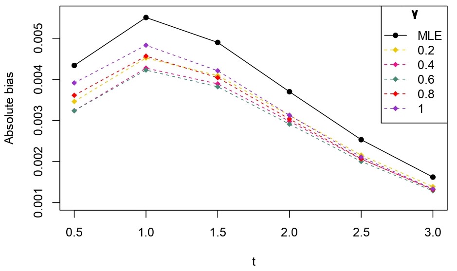
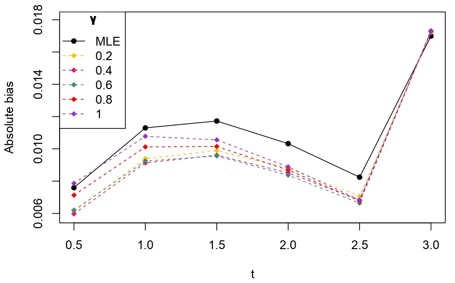
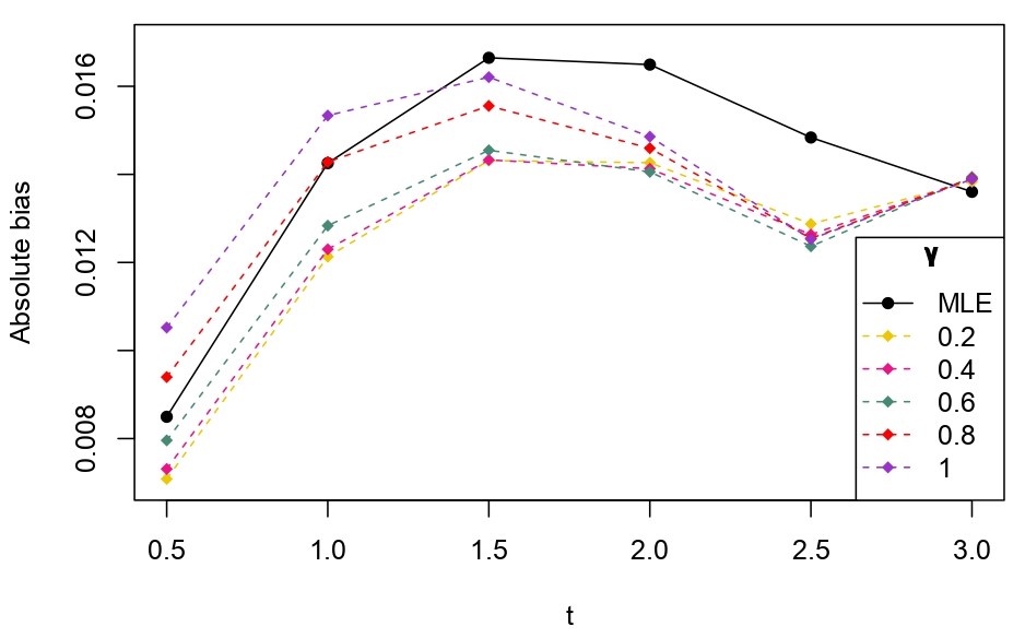
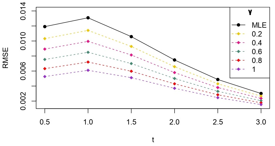
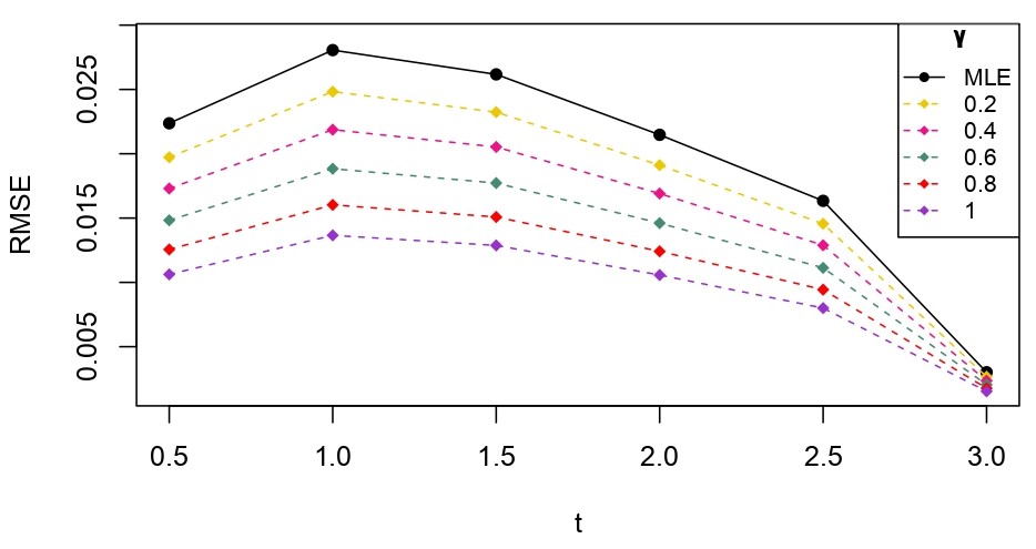
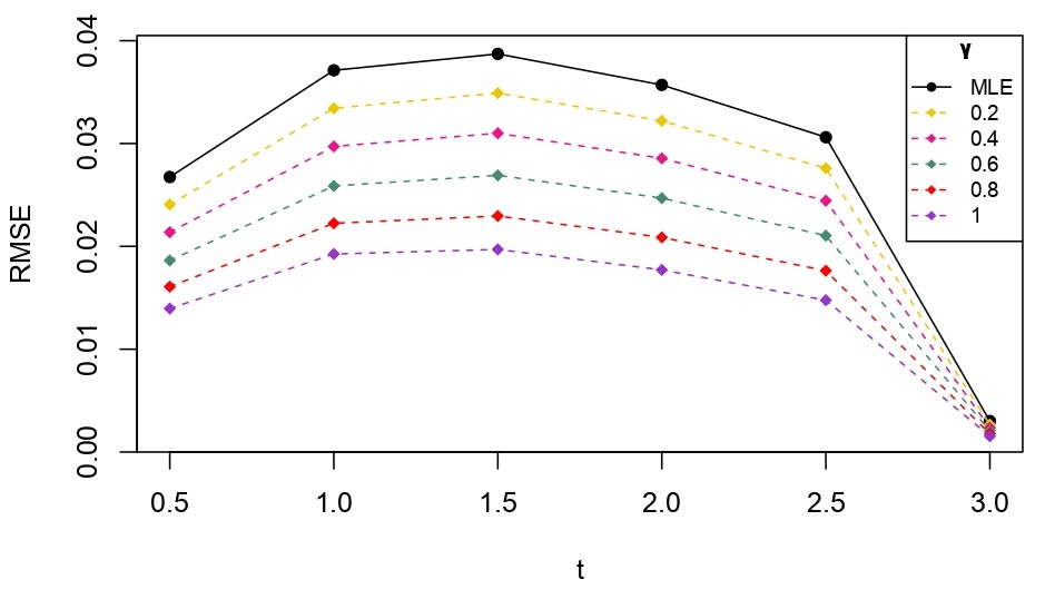
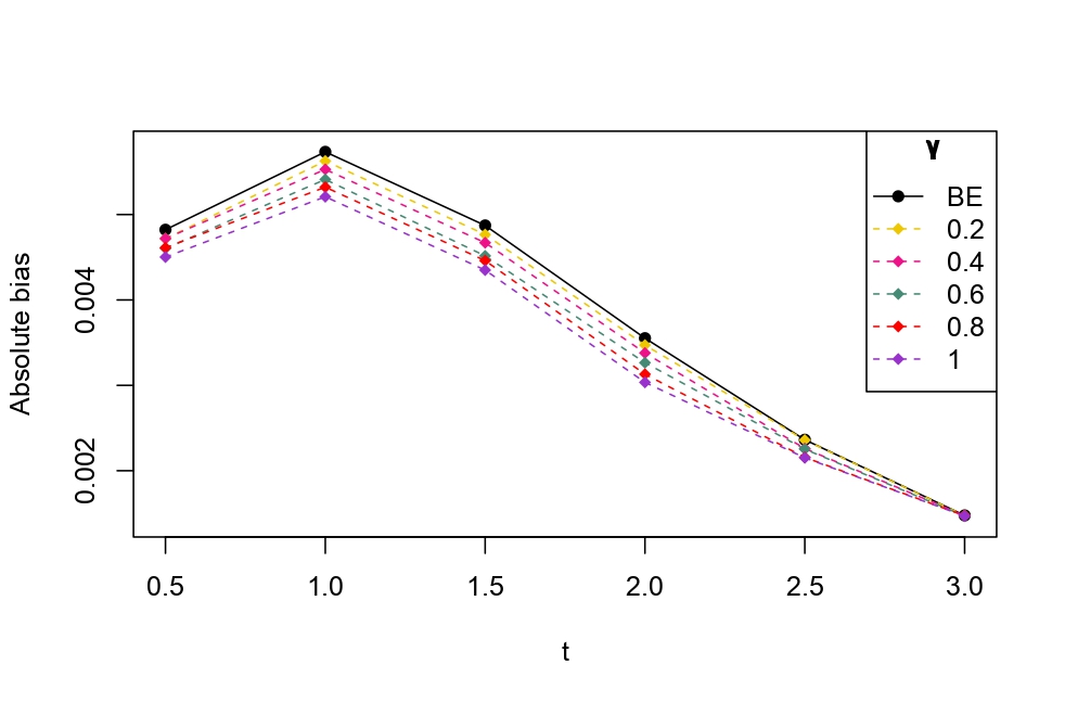
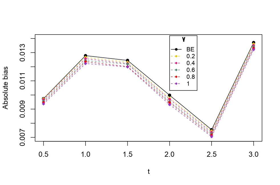
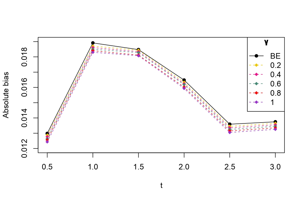
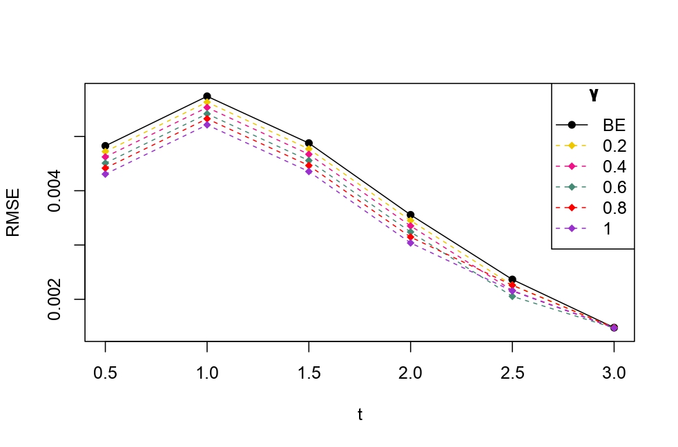
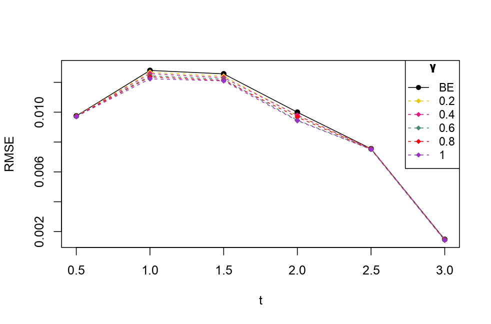
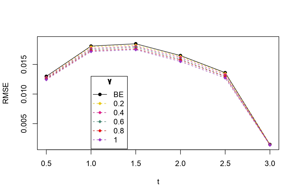
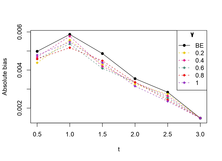
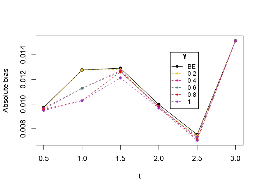
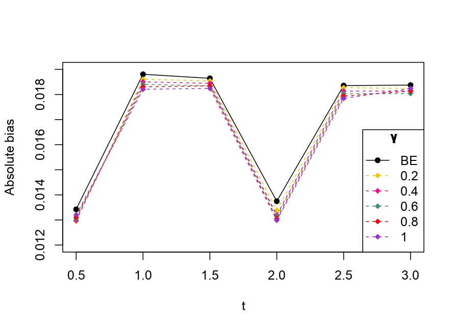
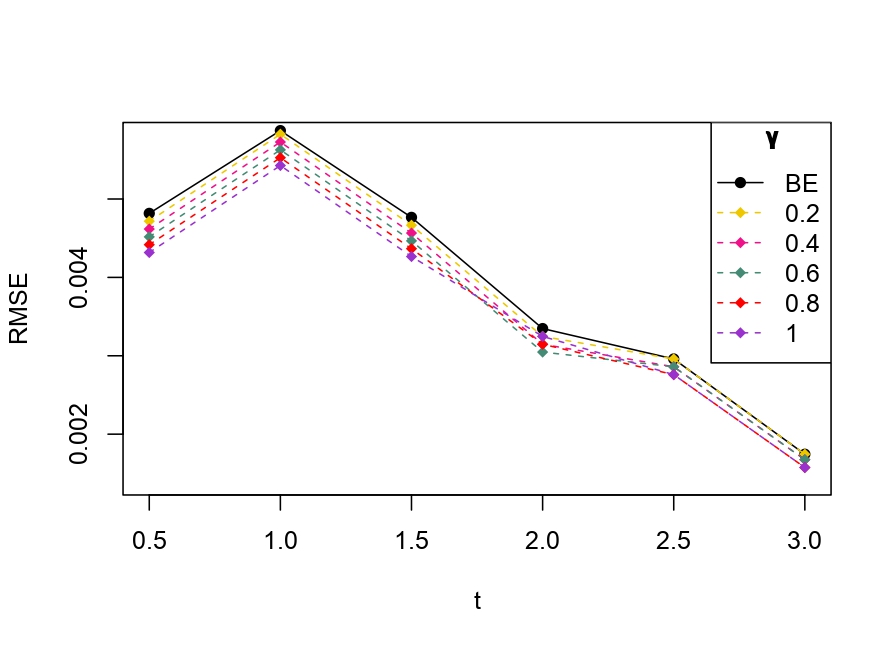
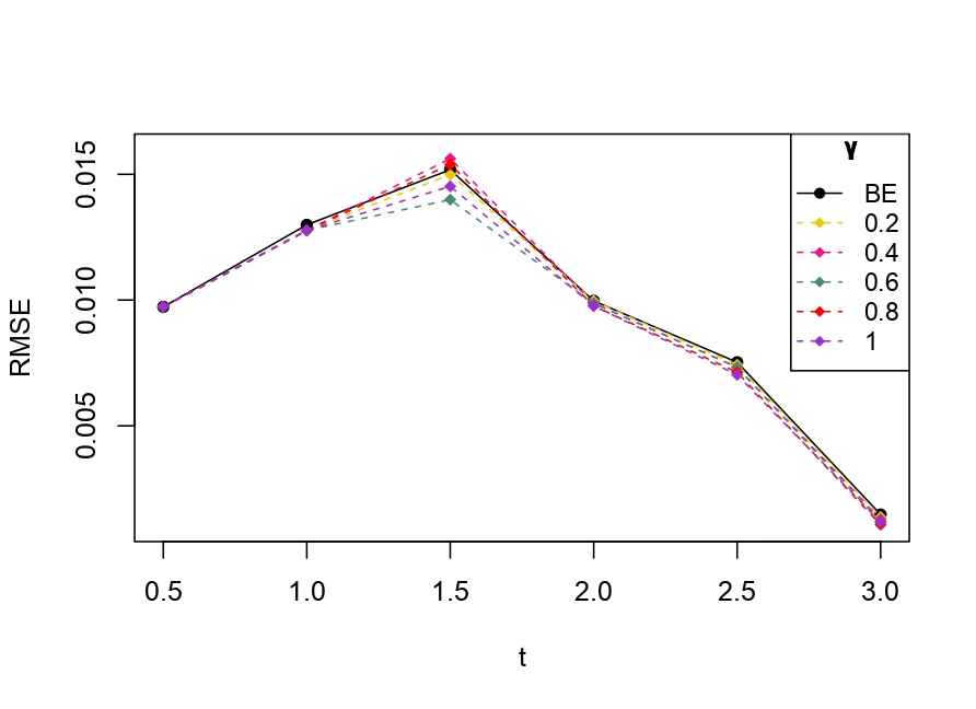
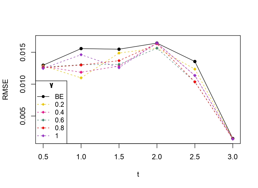
From Table 6.1, it is evident that the bias of MLE is less than that of WMDPDE in pure data. When data is contaminated, WMDPDE performs better than MLE as the bias of WMDPDE is less than that of MLE. Also, the bias change for WMDPDE is lesser than that of MLE, from pure to contamination scheme. Table 6.1 shows that the bias of BE is less than that of WRBE in the pure data scheme. However, after contamination, WRBE shows less bias. Thus, from Tables 6.1 and 6.1, it can be concluded that WMDPDE and WRBE are robust estimators. Further, observing the figures in Tables 6.1 and 6.1, it can be concluded that under contamination, WRBE has the smallest bias compared to other estimates. Hence, if prior information is available, WRBE is the best choice, but if it is not possible to get prior knowledge, one can rely on WMDPDE for robust estimation purposes. Also, absolute bias and RMSE of reliability estimates of parameters for contamination under Sim. 1 setting are represented graphically in Figures 1-3. The superiority of robust estimates under contamination is also clearly visible from these figures.
Bias of BE and WRBE under simulation. Pure Data Contamination Normal Prior BE 0.008511 -0.000794 -0.009001 -0.001089 0.019942 -0.001403 -0.011804 -0.003973 WRBE 0.009226 -0.000977 -0.010004 -0.002014 0.009990 -0.000989 -0.009976 -0.002014 0.009764 -0.001028 -0.009714 -0.001612 0.009985 -0.000989 -0.009996 -0.002013 0.009241 -0.001001 -0.009283 -0.001567 0.010009 -0.000968 -0.009986 -0.001996 0.010006 -0.001013 -0.009824 -0.002014 0.009998 -0.000994 -0.009998 -0.001989 0.009792 -0.000997 -0.009604 -0.001807 0.010025 -0.000981 -0.010016 -0.001973 BE 0.000006 0.009929 -0.000001 0.010009 -0.000073 0.010103 0.000020 0.010031 WRBE 0.000024 0.009955 -0.000013 0.009974 0.000030 0.009968 0.000010 0.009999 -0.000008 0.009980 0.000002 0.009982 0.000014 0.010028 -0.000004 0.010001 0.000009 0.009979 0.000004 0.009969 0.000060 0.009988 0.000006 0.009983 0.000021 0.009938 -0.000013 0.009974 -0.000034 0.009945 -0.000018 0.010008 0.000028 0.010017 -0.000006 0.009972 -0.000047 0.010039 0.000026 0.010022 Dirichlet Prior BE 0.009434 -0.001010 -0.010029 -0.001008 0.012976 -0.001770 -0.010445 -0.002651 WRBE 0.009817 -0.000938 -0.011580 -0.001155 0.010042 -0.001057 -0.009628 -0.001896 0.009707 -0.000934 -0.010160 -0.001812 0.010488 -0.001133 -0.010255 -0.001835 0.009784 -0.001042 -0.009966 -0.002031 0.009584 -0.001216 -0.010399 -0.002060 0.009814 -0.001001 -0.009879 -0.002003 0.009545 -0.000989 -0.009802 -0.002114 0.009836 -0.001000 -0.010015 -0.002000 0.010028 -0.001007 -0.010238 -0.002139 BE 0.000004 0.009158 -0.000019 0.009561 -0.000077 0.012739 -0.000055 0.010048 WRBE -0.000029 0.009476 -0.000019 0.010011 -0.000056 0.010023 0.000026 0.009876 -0.000047 0.009306 -0.000025 0.010022 -0.000053 0.010013 0.000026 0.010028 -0.000020 0.009807 0.000001 0.010011 -0.000046 0.009661 -0.000009 0.009891 -0.000033 0.009550 0.000004 0.010007 -0.000060 0.009721 0.000019 0.010031 -0.000044 0.010016 0.000008 0.009896 -0.000041 0.009893 -0.000008 0.010004
6.2 Influence function analysis
We study the influence of WMDPDE and WRBE as described in section (5). The influence functions are empirically computed for Sim. 1 with tuning parameters and are represented through the Figures 4-5. From these figures, it has been observed that the influence function is bounded, which verifies the robustness of the estimates. Since the bounds for WRBE under normal and Dirichlet prior came out to be similar, the IF figure for
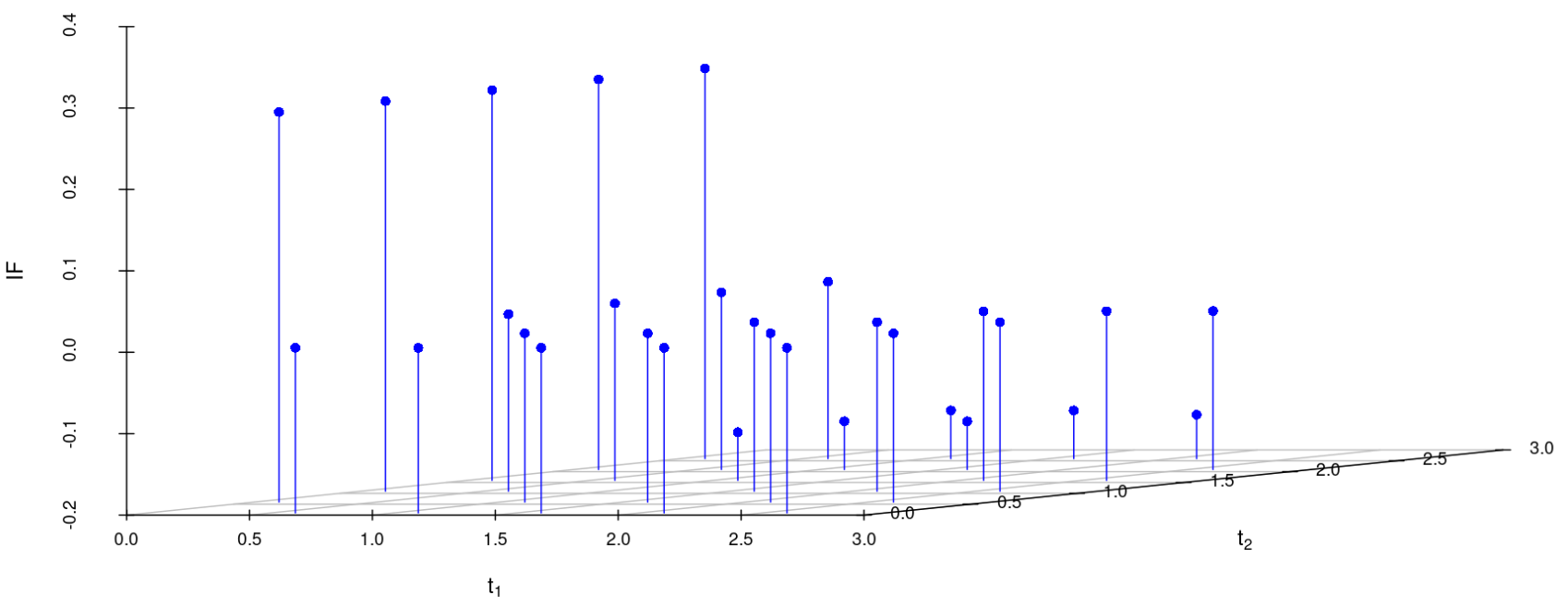
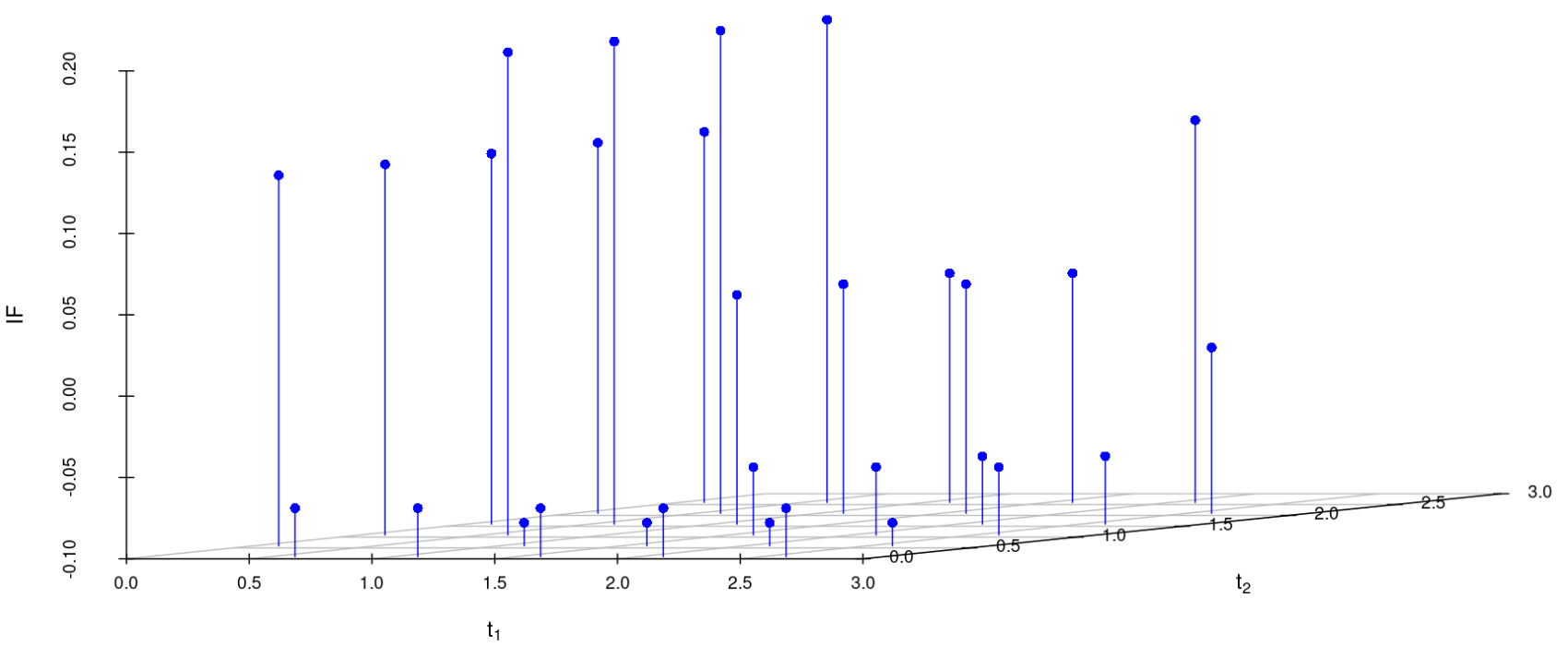
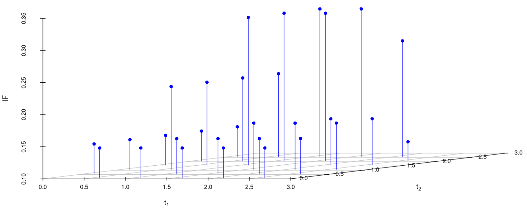
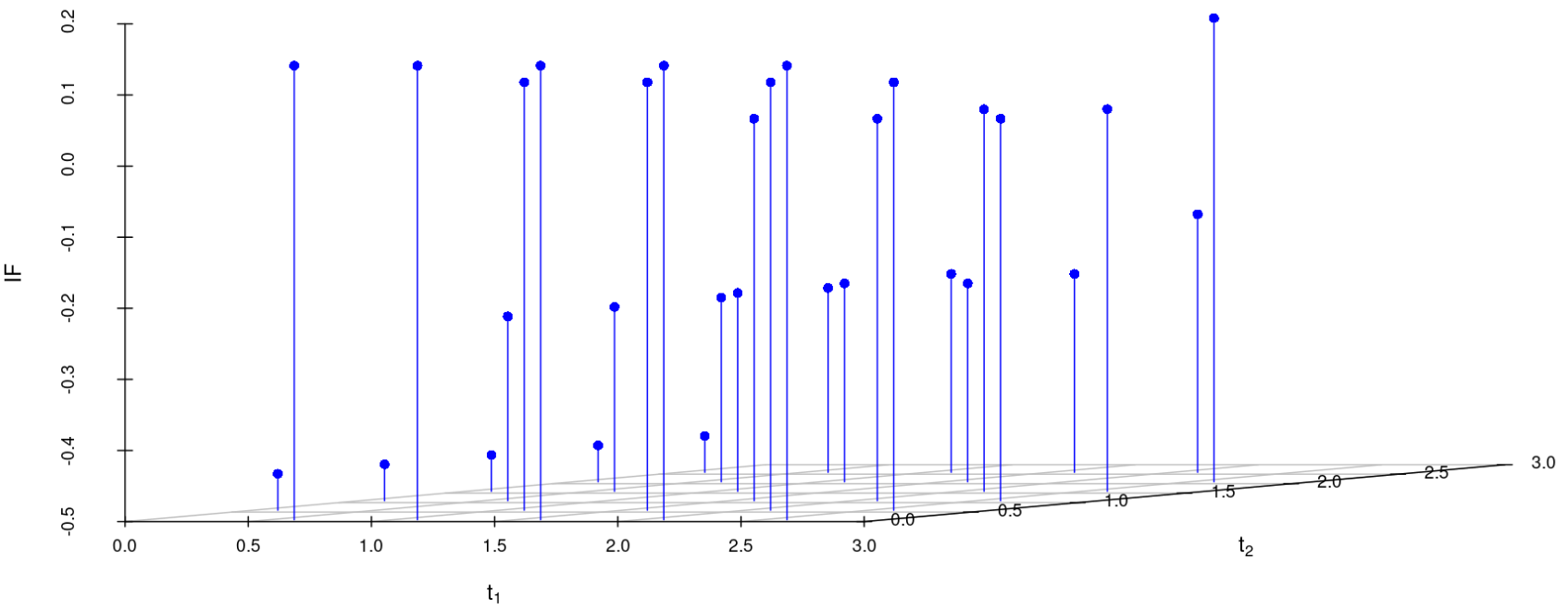
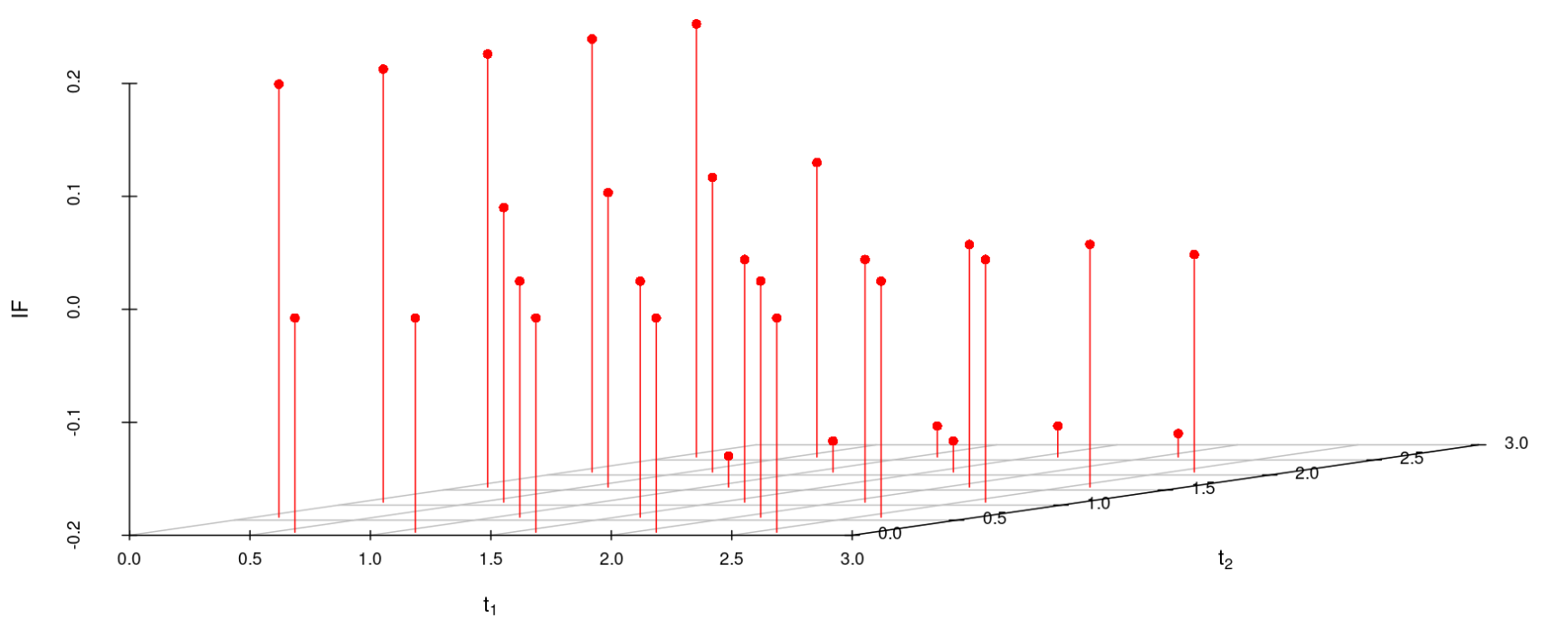
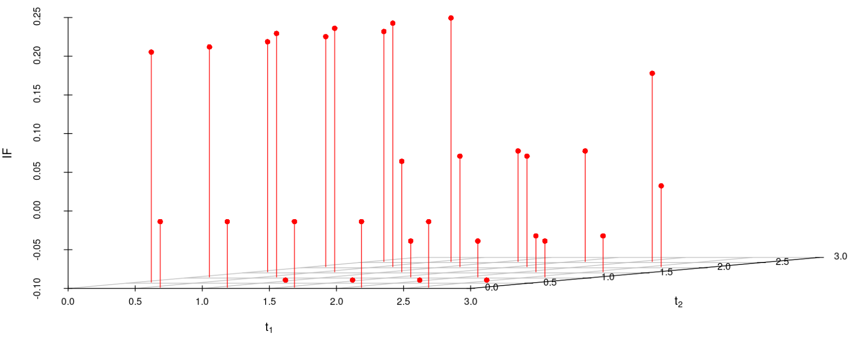
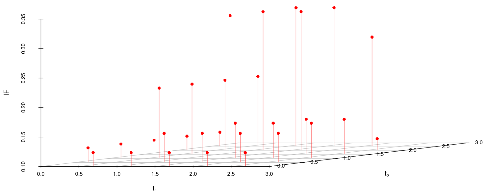
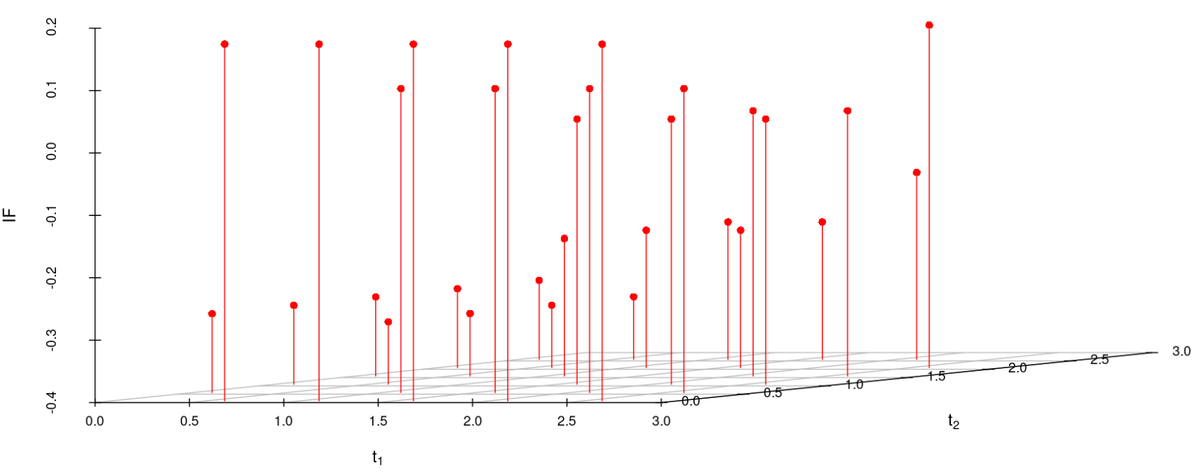
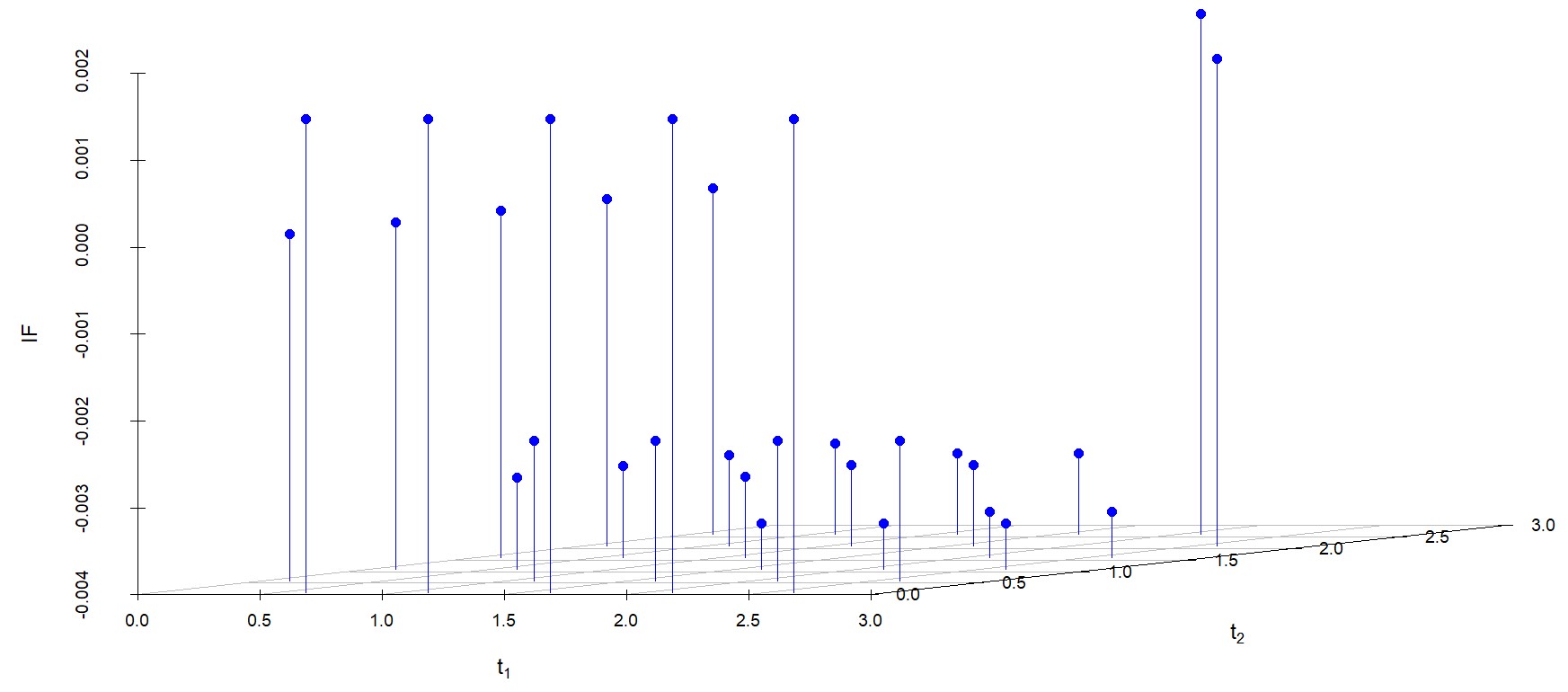
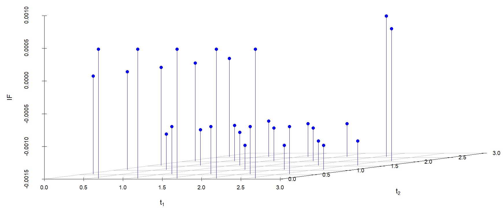
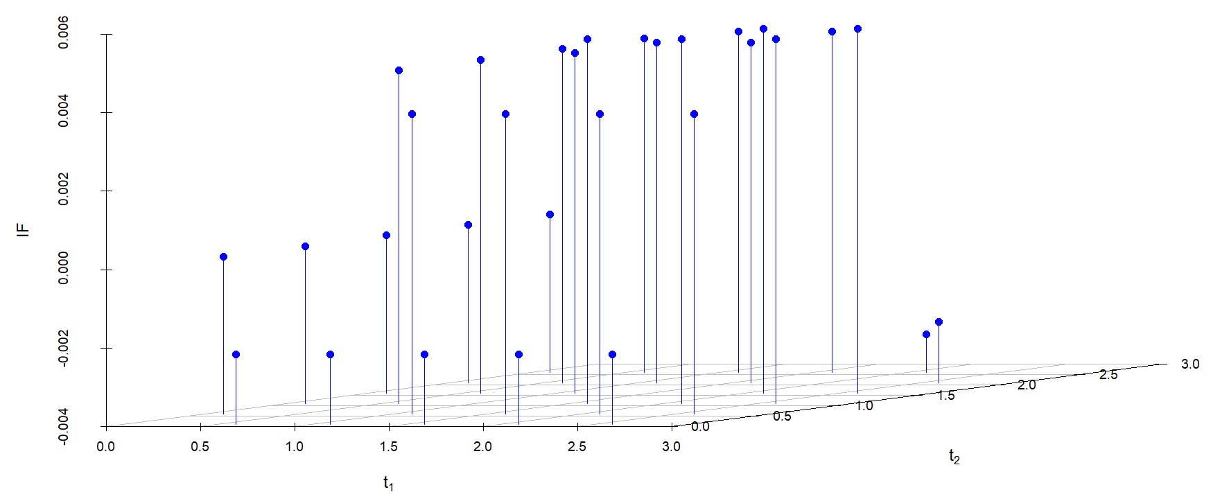
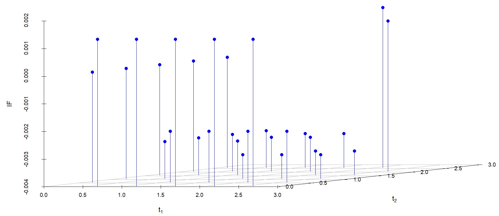
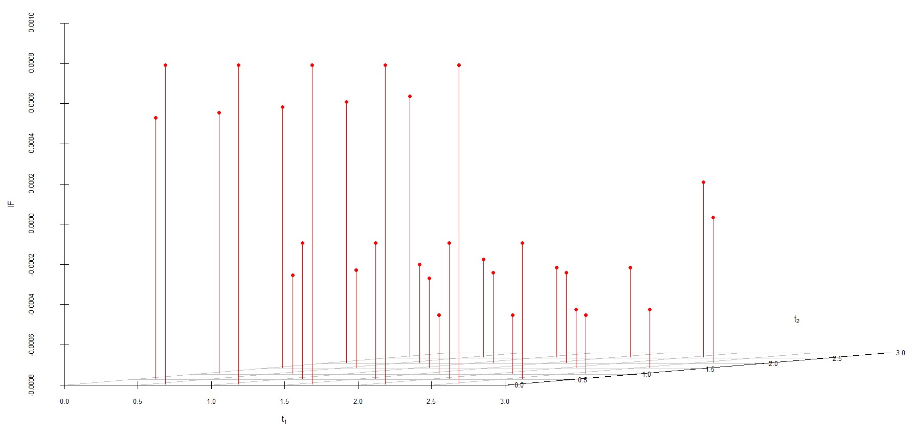
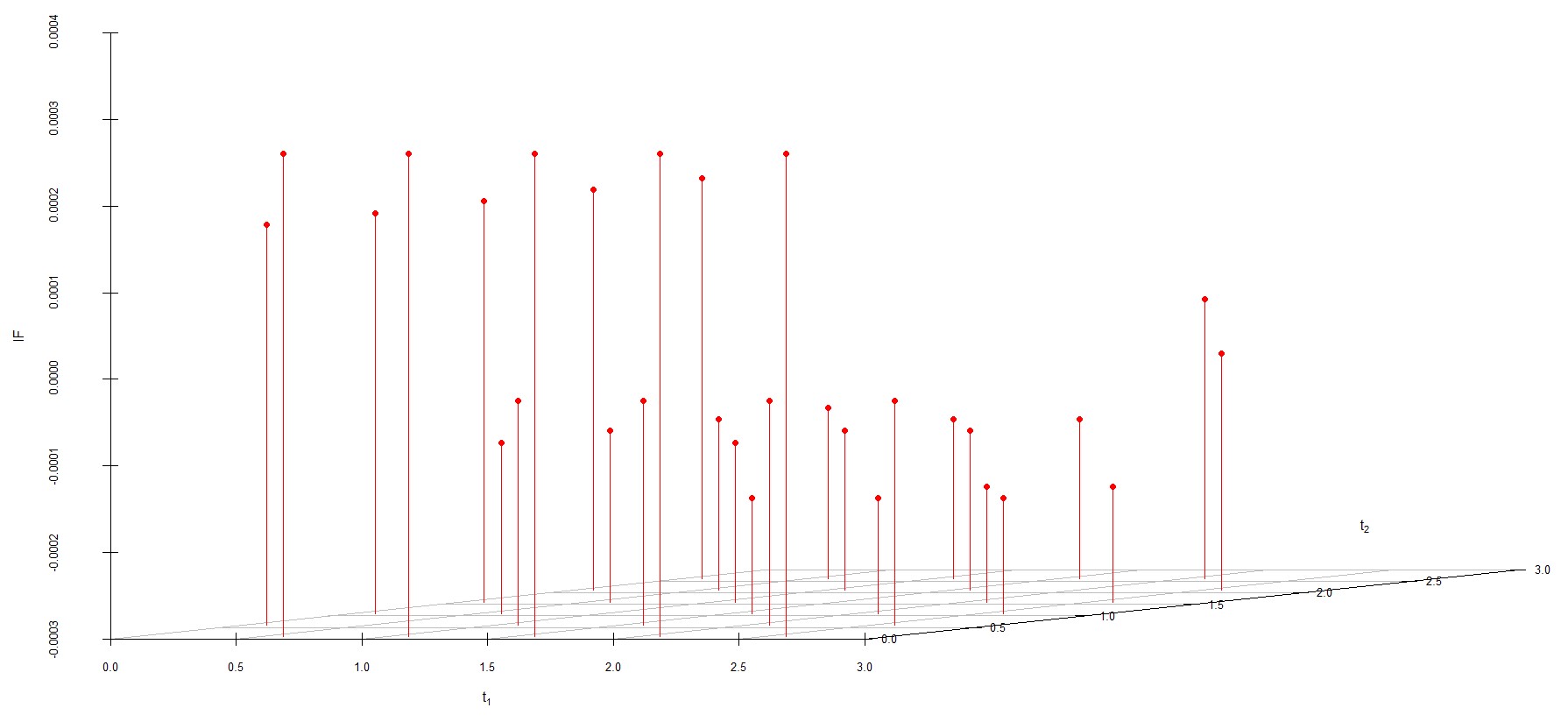
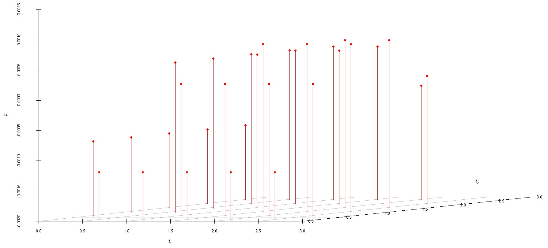
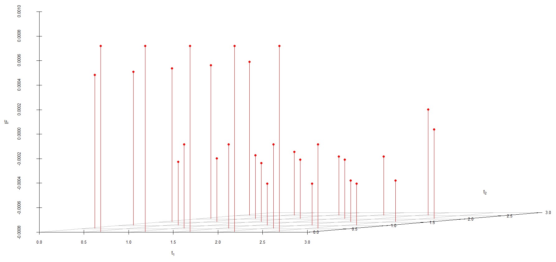
Dirichlet prior is omitted here. Further, the influence function values for WRBE are less than those of WMDPDE for all the parameters. When the tuning parameter value is increased from to , the influence function values for WRBE decrease. Thus, the robustness of WRBE is increased with an increased value of .
6.3 Data Analysis
The application of NOSD test data can be extended to the survival analysis of biomedical data. Therefore, data for the analysis is extracted from the SEER research database (http://www.seer.cancer.gov). The information in this extracted dataset is focused only on patients diagnosed with pancreatic cancer during the year 2016 in the age group 50-55. A total of 235 patients are involved in the study where patient death due to pancreatic cancer is taken as competing cause 1, and death due to other causes is taken as competing cause 2. The size of the tumour is taken as stress level, which is indicated as,
Patients are observed over the months, and deaths are recorded within the follow-up time. The data layout is described in Table 6.3.
Layout of the SEER pancreatic cancer data (www.seer.cancer.gov). Groups Diagnosed Tumor Inspection Times Deaths Survived patients size (Months) (Cancer, Other) Patients 1 69 1 02 10 30 (07,1) (26,0) (28,2) 5 2 90 2 01 10 34 (14,1) (33,1) (31,3) 7 3 76 3 01 08 20 (21,1) (23,1) (22,1) 7
A bootstrap goodness of fit test is performed to ensure that the two-parameter Lindley distribution is fitted to the data. The distance-based test statistic is given as,
where, , , are the empirical and estimated failure or survival probability respectively. For estimation purposes, the initial values found through the grid-search procedure are . MLE given in Table 6.3 is used to obtain the expected number of deaths and survivals. The value of the test statistic came out to be , and the corresponding approximate p-value is , which strongly satisfies the assumption of Lindley distribution as the lifetime distribution. The estimates derived from MLE and WMDPDE with asymptotic confidence interval (CI) are given in Tabel 6.3. Similarly, Bayes estimates (BE) and weighted robust Bayes estimates (WRBE) with Highest posterior density credible interval (HPD CRI) are reported in Table 6.3. The bootstrap bias (BT Bias) and root mean square of error (RMSE) of the estimates are shown in Table 6.3. It can be seen from this table that the BT bias and RMSE of robust estimates are less than those of classical estimates. It is also observed that WRBE has the least bias and RMSE among the four estimation methods, which conforms to the findings of the simulation experiment and aligns with the objective of this study.
Classical estimates (95% Asymp. CI) for real data. Est. (CI) Est. (CI) Est. (CI) Est. (CI) MLE -0.611204 0.198243 0.399344 0.162147 (-0.6249,-0.5974) (0.1951,0.2013) (0.3801,0.4185) (0.1547,0.1695) WMDPDE -0.611665 0.087949 0.440619 0.209047 (-0.6225,-0.6007) (0.0852,0.0906) (0.4184,0.4627) (0.2016,0.2164) -0.600050 0.339492 0.499800 0.100896 (-0.6142,-0.5858) (0.3363,0.3426) (0.4854,0.5141) (0.0939,0.1078) -0.600021 0.339811 0.499956 0.100701 (-0.6133,-0.5866) (0.3366,0.3429) (0.4812,0.5186) (0.0934,0.1079) -0.600009 0.339983 0.499996 0.100549 (-0.6138,-0.5861) (0.3367,0.3431) (0.4674,0.5325) (0.0928,0.1082) -0.600002 0.340070 0.500005 0.100431 (-0.6180,-0.5819) (0.3367,0.3433) (0.4311,0.5689) (0.0917,0.1090)
Bayes estimates (95% HPD CRI) for real data. Est. (CI) Est. (CI) Est. (CI) Est. (CI) Normal prior BE -0.600302 0.339304 0.499718 0.099922 (-0.6049,-0.5958) (0.3341,0.3433) (0.4945,0.5045) (0.0952,0.1041) WRBE -0.599938 0.340171 0.500442 0.099048 (-0.6015,-0.5984) (0.3385,0.3416) (0.4988,0.5020) (0.0972,0.1006) -0.599988 0.339434 0.500200 0.100394 (-0.6014,-0.5984) (0.3378,0.3409) (0.4986,0.5016) (0.0989,0.1019) -0.599946 0.339543 0.499693 0.099116 (-0.6016,-0.5985) (0.3379,0.3412) (0.4980,0.5013) (0.0975,0.1006) -0.600584 0.340366 0.499820 0.100391 (-0.6019,-0.5986) (0.3386,0.3419) (0.4981,0.5012) (0.0985,0.1018) -0.599790 0.340013 0.500456 0.100688 (-0.6012,-0.5981) (0.3385,0.3416) (0.4989,0.5021) (0.0992,0.1022) Dirichlet prior BE -0.600644 0.340258 0.499893 0.100295 (-0.6052,-0.5958) (0.3356,0.3446) (0.4955,0.5052) (0.0953,0.1047) WRBE -0.599988 0.339434 0.500200 0.100394 (-0.6014,-0.5984) (0.3378,0.3409) (0.4986,0.5016) (0.0989,0.1019) -0.599946 0.339543 0.499693 0.099116 (-0.6016,-0.5985) (0.3379,0.3412) (0.4980,0.5013) (0.0975,0.1006) -0.600584 0.340366 0.499820 0.100391 (-0.6019,-0.5986) (0.3386,0.3419) (0.4981,0.5012) (0.0985,0.1018) -0.599790 0.340013 0.500456 0.100688 (-0.6012,-0.5981) (0.3385,0.3416) (0.4989,0.5021) (0.0992,0.1022) -0.600246 0.340003 0.499874 0.099856 (-0.6016,-0.5986) (0.3384,0.3417) (0.4983,0.5013) (0.0981,0.1014)
BT bias and RMSE of the estimates for real data. BT Bias RMSE BT Bias RMSE BT Bias RMSE BT Bias RMSE MLE -0.011560 0.012516 -0.063412 0.075775 -0.056070 0.062076 0.003658 0.004223 WMDPDE -0.005313 0.005974 -0.030313 0.035592 -0.017427 0.019746 0.002893 0.003343 -0.002404 0.002756 -0.013876 0.016206 -0.004721 0.005412 0.002260 0.002611 -0.001099 0.001270 -0.005113 0.005961 -0.001065 0.001227 0.001763 0.002036 -0.000460 0.000533 -0.000489 0.000576 -0.000092 0.000107 0.001377 0.001590 -0.000125 0.000144 0.001814 0.002101 0.000139 0.000161 0.001078 0.001245 Normal Prior BE -0.000862 0.000950 0.000958 0.000859 -0.000747 0.000451 -0.00051 0.000427 WRBE -0.000480 0.000632 -0.000540 0.000678 -0.000426 0.000584 -0.000231 0.000482 0.000578 0.000876 -0.000708 0.000811 0.000581 0.000704 -0.000012 0.000400 0.000003 0.000401 0.000006 0.000395 -0.000142 0.000419 0.000111 0.000408 -0.000516 0.000652 -0.000138 0.000434 -0.000647 0.000765 0.000358 0.000951 0.000354 0.000538 -0.000470 0.000622 -0.000093 0.000424 0.000601 0.000725 Dirichlet Prior BE 0.000931 0.001003 -0.000935 0.001018 -0.000532 0.000430 -0.000813 0.000557 WRBE 0.000062 0.000413 0.000163 0.000438 0.000050 0.000429 0.000453 0.000458 0.000420 0.000585 0.000458 0.000618 -0.0002567 0.000477 0.000505 0.000253 0.000415 0.000575 -0.000443 0.000601 -0.000628 0.000457 0.000191 0.000476 -0.000222 0.000451 -0.000121 0.000402 -0.000369 0.000541 0.000248 0.000436 0.000464 0.000604 0.000314 0.000501 -0.000051 0.000403 0.000311 0.000511
6.4 Testing of Hypothesis Based on Robust Bayes Factor
For the given data in Table (6.3), testing of the hypothesis based on the robust Bayes factor is conducted here. Let us consider a simple null hypothesis against the alternative as follows.
A continuous prior density would lead to zero prior probability to test . Therefore, it is suggestive to take an -neighbourhood (spherical) around . The empirical prior and posterior probabilities are calculated to obtain the empirical Bayes factor. From equation (21), the Bayes factor can be calculated using relation
Here, the simple null hypothesis is taken as and . Table 6.4 shows the empirically calculated Bayes factor for different tuning parameters under Normal and Dirichlet prior.
Empirical value of Bayes factor. Tuning Prior Posterior Bayes Factor Parameter odds odds BF01 Normal prior 0.162790 3.827585 23.51231 5.086957 31.24845 5.363635 32.94804 4.882353 29.99160 4.223880 25.94669 Dirichlet prior 0.147727 5.733331 38.81023 3.929579 26.60022 4.223880 28.59241 4.263158 28.85829 6.769229 45.82246
Since the Bayes factor measures the strength of the evidence the data offers supporting one hypothesis over another, Jeffreys [26] suggested a scale to interpret the Bayes factor and Kass and Raftery [27] simplified it further, which is given in Table 6.4. Observing table 6.4 shows that support for is strong.
Interpretation of Bayes factor [27]. BF01 Support for Negative 1 to 3 Not worth more than a bare mention 3 to 20 Positive 20 to 150 Strong Very Strong
6.5 Optimal Choice of Tuning Parameter
As discussed in the introduction, the DPD measure-based estimation depends on the choice of tuning parameter . Hence, finding the optimal value for tuning the parameter concerning the interest criteria is required. Here, We suggest a non-iterative method based on the approach introduced by Warwick and Jones [41], which involves minimizing the objective function
| (22) |
where, are predefined positive weight values with . For the given data in Table (6.3), under different values of , WMDPDE are obtained and is calculated with From the results presented in Table 6.5, is the optimal value of the tuning parameter in this investigated case.
Optimal value of tuning parameter . 0.10 0.3759697 0.15 0.3688173 0.20 0.4059839 0.25 0.5476472 0.30 0.2162255 0.35 0.2020160 0.40 0.1891334 0.45 0.1775084 0.50 0.1671194 0.55 0.1580054 0.60 0.1502879 0.65 0.1442069 0.70 0.1401766 0.80 0.1413516 0.85 0.1492402 0.90 0.1649594 0.95 0.1920193 1.00 0.2353263
7 Conclusion
This work is focused on studying robust estimation in the Bayesian framework under two competing causes of failures formulated by Lindley’s lifetime distribution in the context of one-shot device data analysis where the robustified posterior density is developed on the exponential form of the maximizer equation based on the density power divergence method. Through extensive simulation experiments, the robustness of the weighted minimum density power divergence estimator (WMDPDE) and weighted robust Bayes estimator (WRBE) has been proved over the conventional maximum likelihood estimator (MLE) and Bayesian estimator (BE), respectively. It has also been found that when data is contaminated, the bias of the WRBE is the least among the four estimation methods. However, when prior information cannot be obtained, one can rely on a WMDPDE. Robust hypothesis testing based on the Bayes factor has also been studied. Further, the influence function, which measures the robustness analytically, has been derived and is shown graphically. Finally, a pancreatic cancer dataset has been taken for real-life lifetime data analysis to establish the utility of the theoretical results explained in this work.
The model analyzed here can be implemented under step stress, assuming other lifetime distributions. This study can be extended to the situation of dependent competing risks. The missing cause of failure analysis can also be conducted. Efforts in this direction are in the pipeline, and we are optimistic about reporting these findings soon.
Disclosure statement
The authors report there are no competing interests to declare.
Data availability statement
Surveillance, Epidemiology, and End Results (SEER) Program (www.seer.cancer.gov) SEER*Stat Database: Incidence - SEER Research Data, 8 Registries, Nov 2021 Sub (1975-2019) - Linked To County Attributes - Time Dependent (1990-2019) Income/Rurality, 1969-2020 Counties, National Cancer Institute, DCCPS, Surveillance Research Program, released April 2022, based on the November 2021 submission.
References
- Abba and Wang, [2023] Abba, B. and Wang, H. (2023). A new failure times model for one and two failure modes system: A bayesian study with hamiltonian monte carlo simulation. Proceedings of the Institution of Mechanical Engineers, Part O: Journal of Risk and Reliability, page 1748006X221146367.
- Abba et al., [2024] Abba, B., Wu, J., and Muhammad, M. (2024). A robust multi-risk model and its reliability relevance: A bayes study with hamiltonian monte carlo methodology. Reliability Engineering & System Safety, page 110310.
- Acharyya et al., [2024] Acharyya, S., Pati, D., Sun, S., and Bandyopadhyay, D. (2024). A monotone single index model for missing-at-random longitudinal proportion data. Journal of Applied Statistics, 51(6):1023–1040.
- [4] Baghel, S. and Mondal, S. (2024a). Analysis of one-shot device testing data under logistic-exponential lifetime distribution with an application to seer gallbladder cancer data. Applied Mathematical Modelling, 126:159–184.
- [5] Baghel, S. and Mondal, S. (2024b). Robust estimation of dependent competing risk model under interval monitoring and determining optimal inspection intervals. Applied Stochastic Models in Business and Industry.
- Balakrishnan and Castilla, [2024] Balakrishnan, N. and Castilla, E. (2024). Robust inference for destructive one-shot device test data under weibull lifetimes and competing risks. Journal of Computational and Applied Mathematics, 437:115452.
- [7] Balakrishnan, N., Castilla, E., Jaenada, M., and Pardo, L. (2023a). Robust inference for nondestructive one-shot device testing under step-stress model with exponential lifetimes. Quality and Reliability Engineering International, 39(4):1192–1222.
- [8] Balakrishnan, N., Castilla, E., Martin, N., and Pardo, L. (2023b). Power divergence approach for one-shot device testing under competing risks. Journal of Computational and Applied Mathematics, 419:114676.
- [9] Balakrishnan, N., Jaenada, M., and Pardo, L. (2022a). Non-destructive one-shot device testing under step-stress model with weibull lifetime distributions. arXiv preprint arXiv:2208.02674.
- [10] Balakrishnan, N., Jaenada, M., and Pardo, L. (2022b). The restricted minimum density power divergence estimator for non-destructive one-shot device testing the under step-stress model with exponential lifetimes. arXiv preprint arXiv:2205.07103.
- [11] Balakrishnan, N., Jaenada, M., and Pardo, L. (2022c). Robust rao-type tests for non-destructive one-shot device testing under step-stress model with exponential lifetimes. In International Conference on Soft Methods in Probability and Statistics, pages 24–31. Springer.
- Balakrishnan et al., [2024] Balakrishnan, N., Jaenada, M., and Pardo, L. (2024). Non-destructive one-shot device test under step-stress experiment with lognormal lifetime distribution. Journal of Computational and Applied Mathematics, 437:115483.
- [13] Balakrishnan, N., So, H. Y., and Ling, M. H. (2015a). Em algorithm for one-shot device testing with competing risks under exponential distribution. Reliability Engineering & System Safety, 137:129–140.
- [14] Balakrishnan, N., So, H. Y., and Ling, M. H. (2015b). Em algorithm for one-shot device testing with competing risks under weibull distribution. IEEE Transactions on Reliability, 65(2):973–991.
- Basu et al., [1998] Basu, A., Harris, I. R., Hjort, N. L., and Jones, M. (1998). Robust and efficient estimation by minimising a density power divergence. Biometrika, 85(3):549–559.
- Calvino et al., [2021] Calvino, A., Martin, N., and Pardo, L. (2021). Robustness of minimum density power divergence estimators and wald-type test statistics in loglinear models with multinomial sampling. Journal of Computational and Applied Mathematics, 386:113214.
- Castilla Gonzalez, [2011] Castilla Gonzalez, E. M. (2011). Robust statistical inference for one-shot devices based on divergences. Universidad Complutense de Madrid, New York.
- Chandra et al., [2024] Chandra, P., Mandal, H. K., Tripathi, Y. M., and Wang, L. (2024). Inference for depending competing risks from marshall–olikin bivariate kies distribution under generalized progressive hybrid censoring. Journal of Applied Statistics, pages 1–30.
- Fan et al., [2009] Fan, T.-H., Balakrishnan, N., and Chang, C.-C. (2009). The bayesian approach for highly reliable electro-explosive devices using one-shot device testing. Journal of Statistical Computation and Simulation, 79(9):1143–1154.
- Ghitany et al., [2008] Ghitany, M. E., Atieh, B., and Nadarajah, S. (2008). Lindley distribution and its application. Mathematics and computers in simulation, 78(4):493–506.
- Ghosh and Basu, [2016] Ghosh, A. and Basu, A. (2016). Robust bayes estimation using the density power divergence. Annals of the Institute of Statistical Mathematics, 68:413–437.
- Ghosh et al., [2006] Ghosh, J. K., Delampady, M., and Samanta, T. (2006). An introduction to Bayesian analysis: theory and methods, volume 725. Springer.
- Hampel et al., [2011] Hampel, F. R., Ronchetti, E. M., Rousseeuw, P. J., and Stahel, W. A. (2011). Robust statistics: the approach based on influence functions. John Wiley & Sons, New York.
- Jeffreys, [1935] Jeffreys, H. (1935). Some tests of significance, treated by the theory of probability. In Mathematical proceedings of the Cambridge philosophical society, volume 31(2), pages 203–222. Cambridge University Press.
- Jeffreys, [1973] Jeffreys, H. (1973). Scientific inference. Cambridge University Press.
- Jeffreys, [1998] Jeffreys, H. (1998). The theory of probability. OuP Oxford.
- Kass and Raftery, [1995] Kass, R. E. and Raftery, A. E. (1995). Bayes factors. Journal of the american statistical association, 90(430):773–795.
- Law, [1986] Law, J. (1986). Robust statistics—the approach based on influence functions.
- Lee and Morris A., [1985] Lee, H. L. and Morris A., C. (1985). A multinomial logit model for the spatial distribution of hospital utilization. Journal of Business & Economic Statistics, 3(2):159–168.
- Lindley, [1958] Lindley, D. V. (1958). Fiducial distributions and bayes’ theorem. Journal of the Royal Statistical Society. Series B (Methodological), pages 102–107.
- Lindley, [1970] Lindley, D. V. (1970). Introduction to probability and statistics. Part, 2:46–58.
- Mazucheli and Achcar, [2011] Mazucheli, J. and Achcar, J. A. (2011). The lindley distribution applied to competing risks lifetime data. Computer methods and programs in biomedicine, 104(2):188–192.
- Monnahan et al., [2017] Monnahan, C. C., Thorson, J. T., and Branch, T. A. (2017). Faster estimation of bayesian models in ecology using hamiltonian monte carlo. Methods in Ecology and Evolution, 8(3):339–348.
- Neal, [1996] Neal, R. M. (1996). Bayesian learning for neural networks. Springer New York, NY.
- Neal et al., [2011] Neal, R. M. et al. (2011). Mcmc using hamiltonian dynamics. Handbook of markov chain monte carlo, 2(11):2.
- Sun et al., [2024] Sun, W., Zhu, X., Zhang, Z., and Balakrishnan, N. (2024). Bayesian inference for laplace distribution based on complete and censored samples with illustrations. Journal of Applied Statistics, pages 1–22.
- Thach and Bris, [2019] Thach, T. T. and Bris, R. (2019). Reparameterized weibull distribution: a bayes study using hamiltonian monte carlo. In Proceedings of the 29th European safety and reliability conference. Singapore: Research Publishing, pages 997–1004.
- Thach and Bris, [2020] Thach, T. T. and Bris, R. (2020). Improved new modified weibull distribution: A bayes study using hamiltonian monte carlo simulation. Proceedings of the Institution of Mechanical Engineers, Part O: Journal of Risk and Reliability, 234(3):496–511.
- Thanh Thach and Briš, [2021] Thanh Thach, T. and Briš, R. (2021). An additive chen-weibull distribution and its applications in reliability modeling. Quality and Reliability Engineering International, 37(1):352–373.
- Thomas and Tu, [2021] Thomas, S. and Tu, W. (2021). Learning hamiltonian monte carlo in r. The American Statistician, 75(4):403–413.
- Warwick and Jones, [2005] Warwick, J. and Jones, M. (2005). Choosing a robustness tuning parameter. Journal of Statistical Computation and Simulation, 75(7):581–588.
- Zhang et al., [2022] Zhang, C., Wang, L., Bai, X., and Huang, J. (2022). Bayesian reliability analysis for copula based step-stress partially accelerated dependent competing risks model. Reliability Engineering & System Safety, 227:108718.
8 Appendices
Appendix A Proof of Result (2)
We denote failure probabilities and survival probability for group as
Thus, and i.e. . For the group, the number of failures between the interval is denoted as, . Again, we define, ; where, . Therefore, . Hence, the WDPD measure in equation (5) ignoring the terms independent of parameters is given as
The proof of the theorem proceeds based on Calvino et al. [16]. The simplified version of the proof in the present context is given in the study of Baghel and Mondal [4],
Appendix B Proof of Result 3
Let us denote
Then, the IF of WRBE can be obtained as
where, is the covariance for posterior distribution.
Appendix C Proof of Result 4
Let us denote
Then, the Influence function of the Bayes factor can be obtained as
where,