and non-standard neutrino interactions
Abstract
We discuss the modes in the context of non-standard neutrino interactions that add incoherently to the SM rates. We consider two scenarios: an additional light neutrino; and neutrino lepton flavour violation. We find that an additional light neutrino that interacts with SM fields via a non-universal can increase by up to a factor of two without conflicting with mixing. This model then predicts rates for up to six times larger than the SM. In the context of neutrino lepton flavour violation mediated by leptoquarks we find that the current experimental upper bounds on are already more constraining than direct bounds from and modes for .
1 Introduction
Rare decays play an important role in understanding the dynamics of the standard model (SM) as well as being a fertile ground for the search for new physics. The decays are amongst the cleanest modes to search for new physics due to their well controlled theoretical uncertainty. Experiments at Belle and Babar have already published upper limits on these modes at 2-3 times the SM rate and further improvement is expected from Belle-II, which can reach a sensitivity on the branching ratios of about 10% with 50 ab-1 [1]. Interesting constraints for certain BSM physics can be obtained already with current bounds.
We consider two types of models that add incoherently to the SM rates. First we entertain the possibility of a fourth light neutrino that couples to SM fields through a non-universal . We find that existing constraints on the model allow enhancements of the rates by up to factors of two and that these are correlated with the mode which could reach a rate up to six times larger than in the SM.
We then consider possible contributions from neutrino flavour violating final states in the context of scalar and vector leptoquarks. These contributions are correlated to the charged lepton flavour violating (CLFV) modes and and we find that the current limits on are more restrictive for modes with tau-leptons. The leptoquark scenario also correlates to the neutral and charged B anomalies, as has been extensively discussed in the literature, and we comment on this.
Within the SM the effective Hamiltonian responsible for the transitions originates at lowest order from box and penguin diagrams and is usually written as [2]
| (1) |
with an accurately known Wilson coefficient that is independent of the neutrino flavour and that including NLO QCD corrections [3] and two-loop electroweak corrections [4] is given by
| (2) |
Typical SM predictions obtained with flavio are111These numbers agree within errors with published numbers as in [5, 1]. Neglecting isospin breaking, the neutral and charged modes have the same rates so we choose to present the two modes with the strongest experimental limits.
| (3) |
We list the best current experimental constraints on these modes in Table 1.
| Mode | 90% c.l upper limit | Reference |
|---|---|---|
| Babar [6] | ||
| Belle [7] | ||
| Belle [8] | ||
| Belle [8] |
Belle-II is expected to improve these limits, and has produced a preliminary result at the 90% confidence level [9]. They have averaged this result with the previous ones to arrive at [9]. For the channel, Belle has also combined the charged and neutral modes to obtain the limit [8] but here we will use the limit in Table 1. These results are usually presented as ratios, for which we obtain
| (4) |
The second number is simply the ratio of the limit in Table 1 and the central value in Eq. 3 and somewhat lower than what is used in [10].
2 Effective Hamiltonian at the scale
We can parameterise any new physics relevant for these decays through an effective Hamiltonian at the mass scale. The effective theory originates in extensions of the SM containing new particles at or above the electroweak scale that have been integrated out. In general, this results in additional contributions to in Eq. 2 as well as in new operators. Because our discussion is tied to two types of models, we only need to consider the following
| (5) |
where the operators are
| (6) |
The Wilson coefficients are defined so that they only contain NP contributions and the SM is counted separately through Eq. 2. The list in Eq. 6 includes , , which contribute to . It excludes operators with scalar and tensor neutrino bi-linears that have been considered in [10] because they do not appear in the models we discuss. The operators with charged leptons appear in the models we discuss with coefficients that are related to . The flavour diagonal operators affect decays including the anomalies and have been studied extensively in that context.
We can classify the contributions to from these operators into two types: those that interfere with the SM, ; and those that do not, and . In only the vector current enters the hadronic matrix element so that the contributions to the rate from and are the same. Similarly for those from and . At the same time, the different neutrino chirality eliminates interference between the primed and un-primed-operators for massless neutrinos. The only operators that interfere with the SM are thus the diagonal ones (in neutrino flavour) and . The rates can be evaluated numerically using [11], and the central value (uncertainty will be shown in the figures) is given approximately by
| (7) |
In both the vector and axial-vector currents enter the hadronic matrix element resulting in different contributions for and as well as for and . Numerically, the rate is approximately given by
| (8) |
The parametric uncertainty in these predictions, as estimated by flavio is illustrated in Fig. 1222The uncertainty in these predictions is around 15% and is mostly due to the form factors for the and hadronic transitions, which are responsible for about 10%, while the value of contributes an additional 5%.. We show as a function of (the figure is identical for ) and as a function of (the figure is identical for and ). The red band marks the experimental combination [9] and the green band the SM in Eq. 3 at 1. For we show the dependence on (same for all ), (same for all ) and (same for all and ). In this case the red line shows the 90% c.l. experimental upper bound from Table 1 and the green band the SM at 1.
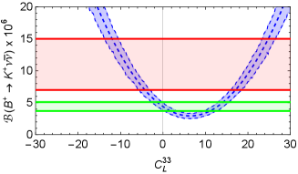
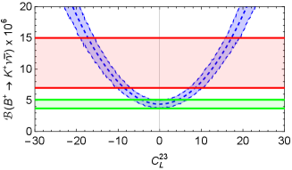
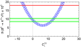
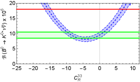
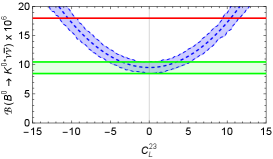
For example, new physics contributions allowed by the value of in Eq. 7 at the 1 level and taking only one non-zero parameter at a time are shown in Table 2 and can also be read off Fig. 1.
| Mode | or | ||
|---|---|---|---|
| or | or | ||
3 An additional light neutrino
The first type of new physics we consider that can increase the SM value of consists of new light neutrinos. In fact, modes with neutrino pairs in the final state count the number of light neutrinos in the SM due to lepton universality. The existence of new light neutrinos is severely constrained by measurements of the invisible width and by cosmological considerations. Assuming lepton universality, the former implies that [12]. Cosmological constraints depend on other parameters and, for example, for a Hubble constant km/s/Mpc [13].
It is possible to avoid these limits with a light sterile neutrino that interacts with the SM through a . The contribution of this neutrino to the width neutrino count is proportional to the square of the mixing parameter and can thus be negligibly small. In addition, if the is non-universal and couples predominantly to the third generation SM fermions, the new neutrino reaches thermal equilibrium with SM particles at a temperature near the -lepton mass. However, at the time of big-bang nucleosynthesis the temperature is about 1 MeV and this difference results in a suppression of the contribution of this neutrino to to a safe level, [14].
We have previously constructed a detailed example of a model with these properties [15, 16] so we do not repeat the details here. The is responsible for two new operators that contribute to and to [17]:
| (9) |
In the notation of Eq. 5, the Wilson coefficients that result in this model are thus:
| (10) |
The first operator in Eq. 9 originates in a flavour changing tree-level exchange of the . The parameters that appear in this result are: the mass; a ratio parameterising the strength of the new interaction relative to the weak interaction, ; and two elements of the matrix that rotates the down-type quarks between the weak and the mass bases. The second operator in Eq. 9 arises from a new penguin diagram and depends on details of the scalar sector through the Inami-Lim function [18]. The existing constraints on these parameters can be summarised as:
- •
-
•
mixing constrains and [17]. Both the SM calculation and the experimental situation regarding have changed significantly so we repeat that analysis here.
In terms of the parameters of interest, the effective Hamiltonian below the scale is:
| (12) |
with the usual operators:
| (13) |
QCD renormalisation group running modifies the Wilson coefficients and introduces one more operator at the scale, . Making use of flavio once more, we find
| (14) |
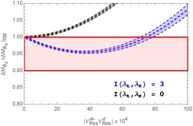
The current experimental average [20] combined with a recent SM prediction [21] results in and we compare this ratio to the prediction of Eq. 14 in Fig. 2 for and . These two values were chosen because a scan over the parameters in the model [18] suggests as a range for the Inami-Lim function. The allowed range for , assuming that is real, is then showed in the right panel of Fig. 2. The key point is that the tree level exchange tends to increase over its SM value and this is severely constrained by current data. It is the new penguin contribution to and that allows to drift below its SM value. As can be seen from Eq. 14, allowing to have a phase can augment the allowed parameter range but a complete phenomenological study of this general case is beyond the scope of the present work.
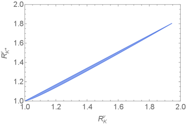
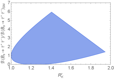
The allowed region in shown in Fig. 2 results in an increase of the rates over their SM value and this is shown in the left panel of Fig. 3. The figure indicates a near perfect correlation between the two neutrino modes and the largest values, near two, are obtained for the upper-right corner of the region in Fig. 2. Interestingly, the same model with the constraint of Eq. 11 can no longer enhance modes by more than a few percent.333In the notation of [22] it predicts . The main difference between these two cases is the strong constraint on (from mixing) that enters in place of which can be close to one.
The model predicts through Eq. 10 a correlation between modes and . The latter currently only has a weak experimental limit from LHCb at 95%c.l. [23]. The prediction can be written in a very simple form because only the hadronic axial vector current contributes,
| (15) |
The allowed parameter region seen in Fig. 2, combined with [3], implies that the model allows
| (16) |
This can be read off Fig. 3 which illustrates the correlation with . On the other hand, the model also allows for where the is significantly suppressed with respect to its SM value.
The corresponding Wilson coefficients affecting the modes exhibiting anomalies, are suppressed with respect to by factors which can be very small [24]. For this reason, this model yields predictions for processes that are very similar to the SM. Correlations between these dimuon modes and modes have also been explored in other models [25, 26].
4 Models with leptoquarks
In this section we consider models that can increase by producing final states with neutrino pairs of different lepton flavour, but with only the three SM neutrinos. The starting point is then scalar and vector leptoquarks with couplings to SM fermions which include a left-handed neutrino of any flavour. They are [27, 28] ,
| (17) |
where the leptoquark fields and their transformation properties under the SM group are given by
| (20) | ||||
| (23) |
Exchange of these particles at tree-level, assuming leptoquark multiplets that are degenerate in mass, generates the following effective Lagrangian
| (24) |
If the fermions in Eq. 24 are in their weak eigenstate basis, rotation to the mass eigenstate basis will introduce mixing angles. Here we will work with defined in a basis in which the down-type fermions are already mass eigenstates [29]. The and up-type quarks need to be further rotated by , and respectively. However, since the neutrino flavour is not measured, working in either their weak or mass basis yields the same results. Collecting the Wilson coefficients for Eq. 6 gives,
| (25) |
All of these leptoquarks contribute to but their contributions are correlated with different modes [30, 31, 32, 33]. We begin with the lepton flavour number violating case which adds incoherently to the SM values for . There are several CLFV modes with existing experimental upper bounds and we list them in Table 3. The corresponding predictions using Eq. 25 are
| (26) |
The best current experimental bounds on these modes as given in [20] are listed in Table 3 along with the constraints they impose on the Wilson coefficients taken one non-zero at a time.
| Mode | 90% c.l | one | or |
|---|---|---|---|
| at a time | |||
| 7.4 | 7.4 | ||
| 44 | 44 | ||
| 0.6 | 0.4 | ||
| 36 | 25 | ||
| 49 | 35 | ||
| 7.4 | 5.2 | ||
| 2.6 | 1.8 |
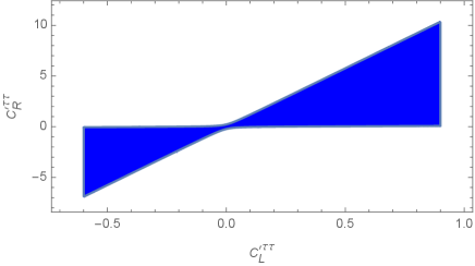
The minimal set of Wilson coefficients consistent with the leptoquark origin of Eq. 25 implies more than one non-zero Wilson coefficient at a time, either , or , . Both situations result in the same bound due to the symmetry between primed and unprimed coefficients in Eq. 26. Without additional assumptions on the leptoquark couplings, in particular allowing to differ from the tightest bounds that follow in this case are shown in the last column of Table 3.
To explore the connection with it is useful to consider Eq. 25 for each leptoquark multiplet separately. We see that only produces and is therefore not correlated with CLFV modes. and generate and whereas and induce and resulting in all cases in . To study the numerical implications of these predictions we consider one lepton flavour pair at a time and present the results in Table 4. These numbers indicate that the CLFV are currently less restrictive on these leptoquark couplings than , Eq. 4, except for the modes.
| LQ | upper bound on | |||||
|---|---|---|---|---|---|---|
| 1.001 | 6.4 | 11 | ||||
| 1.001 | 6.4 | 11 | ||||
| 1.0003 | 2.4 | 3.5 | ||||
| 1.001 | 6.4 | 11 | ||||
| 1.005 | 23 | 40 | ||||
4.1 The B anomalies
Leptoquark models have been studied extensively in the context of the B anomalies and we comment on that here. The neutral B anomalies are observed in modes, and Eq. 24 shows that, with the exception of , these leptoquarks correlate with operators. In particular
| (27) |
Extensive fits to data from modes induced by indicate that [34]444The precise number varies depending on the fit, a more recent one gives -0.41 instead [35]. is a possible solution whereas is not [36]. This implies that
| (28) |
and for .
In a similar manner correlates with and therefore relates to the so-called charged B-anomalies, . We use the latest experimental and theoretical averages from [37] (adding errors in quadrature and using their arithmetic average of theoretical results) in terms of the ratios
| (29) |
Depending on the neutrino lepton flavour, the operator will interfere or not with the SM and both cases were considered in [38, 39]. The results are
| (30) |
The correlations simplify at leading order in CKM angles, where the term with dominates resulting in,
| (31) |
Taking one non-zero parameter at a time for this case, and assuming that the leptoquark contribution results in the central value of Eq. 29 requires or , both much larger than allowed by as quantified in Table 2. Equivalently, the most favourable scenario from Table 2, would result in
| (32) |
More complex leptoquark scenarios have been invoked in the study of the B anomalies where it is possible to avoid a conflict with [40, 41].
5 Summary
We have studied the modes in the context of non-standard neutrino interactions. We first considered a model with an additional light neutrino that couples to a non-universal and found that it can result in close to two. The same model can also enhance by up to a factor six over the SM within the parameter range allowed by mixing and non-production of the at LHC.
Next we considered augmenting through neutrino lepton flavour violating modes. We parameterised this possibility through scalar and vector leptoquark exchange. This type of model correlates with CLFV modes and and we found that the former is currently more restrictive than and CLFV modes.
Finally we briefly commented on the correlation with the B anomalies. In this case we saw that global fits to modes constrain for and leptoquarks so that, by itself, it cannot add more than 10% to . Similarly, current measurements of constrain the parameters of couplings so that can be at most 1.06.
Acknowledgments
This work was supported in part by the Australian Government through the Australian Research Council. XGH was supported in part by Key Laboratory for Particle Physics, Astrophysics and Cosmology, Ministry of Education, Shanghai Key Laboratory for Particle Physics and Cosmology (Grant No. 15DZ2272100), in part by the NSFC (Grant Nos. 11735010, 11975149, and 12090064), and also supported in part by the MOST (Grant No. MOST 106-2112-M-002-003-MY3 ).
References
- [1] Belle-II collaboration, W. Altmannshofer et al., The Belle II Physics Book, PTEP 2019 (2019) 123C01, [1808.10567].
- [2] G. Buchalla, A. J. Buras and M. E. Lautenbacher, Weak decays beyond leading logarithms, Rev. Mod. Phys. 68 (1996) 1125–1144, [hep-ph/9512380].
- [3] G. Buchalla and A. J. Buras, The rare decays , and : An Update, Nucl. Phys. B548 (1999) 309–327, [hep-ph/9901288].
- [4] J. Brod, M. Gorbahn and E. Stamou, Two-Loop Electroweak Corrections for the Decays, Phys. Rev. D83 (2011) 034030, [1009.0947].
- [5] T. Blake, G. Lanfranchi and D. M. Straub, Rare Decays as Tests of the Standard Model, Prog. Part. Nucl. Phys. 92 (2017) 50–91, [1606.00916].
- [6] BaBar collaboration, J. P. Lees et al., Search for and invisible quarkonium decays, Phys. Rev. D 87 (2013) 112005, [1303.7465].
- [7] Belle collaboration, O. Lutz et al., Search for with the full Belle data sample, Phys. Rev. D 87 (2013) 111103, [1303.3719].
- [8] Belle collaboration, J. Grygier et al., Search for decays with semileptonic tagging at Belle, Phys. Rev. D 96 (2017) 091101, [1702.03224].
- [9] Belle-II collaboration, F. Dattola, Search for decays with an inclusive tagging method at the Belle II experiment, in 55th Rencontres de Moriond on Electroweak Interactions and Unified Theories, 5, 2021. 2105.05754.
- [10] T. E. Browder, N. G. Deshpande, R. Mandal and R. Sinha, Impact of measurements on beyond the Standard Model theories, 2107.01080.
- [11] D. M. Straub, flavio: a Python package for flavour and precision phenomenology in the Standard Model and beyond, 1810.08132.
- [12] ALEPH, DELPHI, L3, OPAL, SLD, LEP Electroweak Working Group, SLD Electroweak Group, SLD Heavy Flavour Group collaboration, S. Schael et al., Precision electroweak measurements on the resonance, Phys. Rept. 427 (2006) 257–454, [hep-ex/0509008].
- [13] J. L. Bernal, L. Verde and A. G. Riess, The trouble with , JCAP 1610 (2016) 019, [1607.05617].
- [14] A. D. Dolgov, Neutrinos in cosmology, Phys. Rept. 370 (2002) 333–535, [hep-ph/0202122].
- [15] X.-G. He and G. Valencia, The decay asymmetry and left-right models, Phys. Rev. D66 (2002) 013004, [hep-ph/0203036].
- [16] X.-G. He and G. Valencia, Lepton universality violation and right-handed currents in , Phys. Lett. B779 (2018) 52–57, [1711.09525].
- [17] X.-G. He and G. Valencia, B(s) - anti-B(s) Mixing constraints on FCNC and a non-universal Z-prime, Phys. Rev. D74 (2006) 013011, [hep-ph/0605202].
- [18] X.-G. He and G. Valencia, and FCNC from non-universal bosons, Phys. Rev. D70 (2004) 053003, [hep-ph/0404229].
- [19] A. Hayreter, X.-G. He and G. Valencia, LHC constraints on that couple mainly to third generation fermions, Eur. Phys. J. C 80 (2020) 912, [1912.06344].
- [20] Particle Data Group collaboration, P. A. Zyla et al., Review of Particle Physics, PTEP 2020 (2020) 083C01.
- [21] L. Di Luzio, M. Kirk, A. Lenz and T. Rauh, theory precision confronts flavour anomalies, JHEP 12 (2019) 009, [1909.11087].
- [22] X.-G. He, G. Valencia and K. Wong, Constraints on new physics from , Eur. Phys. J. C78 (2018) 472, [1804.07449].
- [23] LHCb collaboration, R. Aaij et al., Search for the decays and , Phys. Rev. Lett. 118 (2017) 251802, [1703.02508].
- [24] X.-G. He and G. Valencia, decays with leptons in nonuniversal left-right models, Phys. Rev. D87 (2013) 014014, [1211.0348].
- [25] W. Altmannshofer, A. J. Buras, D. M. Straub and M. Wick, New strategies for New Physics search in , and decays, JHEP 04 (2009) 022, [0902.0160].
- [26] S. Descotes-Genon, S. Fajfer, J. F. Kamenik and M. Novoa-Brunet, Implications of anomalies for future measurements of and , Phys. Lett. B 809 (2020) 135769, [2005.03734].
- [27] A. J. Davies and X.-G. He, Tree Level Scalar Fermion Interactions Consistent With the Symmetries of the Standard Model, Phys. Rev. D 43 (1991) 225–235.
- [28] S. Davidson, D. C. Bailey and B. A. Campbell, Model independent constraints on leptoquarks from rare processes, Z. Phys. C 61 (1994) 613–644, [hep-ph/9309310].
- [29] N. G. Deshpande and A. Menon, Hints of R-parity violation in B decays into , JHEP 01 (2013) 025, [1208.4134].
- [30] X.-G. He, J. Tandean and G. Valencia, Charged-lepton-flavor violation in hyperon decays, JHEP 07 (2019) 022, [1903.01242].
- [31] X.-G. He, J. Tandean and G. Valencia, Lepton-flavor-violating semileptonic decay and , Phys. Lett. B797 (2019) 134842, [1904.04043].
- [32] J.-Y. Su and J. Tandean, Exploring leptoquark effects in hyperon and kaon decays with missing energy, Phys. Rev. D 102 (2020) 075032, [1912.13507].
- [33] R. Mandal and A. Pich, Constraints on scalar leptoquarks from lepton and kaon physics, JHEP 12 (2019) 089, [1908.11155].
- [34] M. Algueró, B. Capdevila, A. Crivellin, S. Descotes-Genon, P. Masjuan, J. Matias et al., Emerging patterns of New Physics with and without Lepton Flavour Universal contributions, Eur. Phys. J. C 79 (2019) 714, [1903.09578].
- [35] W. Altmannshofer and P. Stangl, New Physics in Rare B Decays after Moriond 2021, 2103.13370.
- [36] S. Descotes-Genon, L. Hofer, J. Matias and J. Virto, Global analysis of anomalies, JHEP 06 (2016) 092, [1510.04239].
- [37] HFLAV collaboration, Y. S. Amhis et al., Averages of -hadron, -hadron, and -lepton properties as of 2018, Eur. Phys. J. C81 (2021) 226, [1909.12524].
- [38] N. G. Deshpande and X.-G. He, Consequences of R-parity violating interactions for anomalies in and , Eur. Phys. J. C 77 (2017) 134, [1608.04817].
- [39] P. S. Bhupal Dev, A. Soni and F. Xu, Hints of Natural Supersymmetry in Flavor Anomalies?, 2106.15647.
- [40] M. Bauer and M. Neubert, Minimal Leptoquark Explanation for the , , and Anomalies, Phys. Rev. Lett. 116 (2016) 141802, [1511.01900].
- [41] Y. Cai, J. Gargalionis, M. A. Schmidt and R. R. Volkas, Reconsidering the One Leptoquark solution: flavor anomalies and neutrino mass, JHEP 10 (2017) 047, [1704.05849].