Rigidity of pressures of Hölder potentials and the fitting of analytic functions via them
Abstract.
The first part of this work is devoted to the study of higher differentials of pressure functions of Hölder potentials on shift spaces of finite type. By describing the differentials of pressure functions via the Central Limit Theorem for the associated random processes, we discover some rigid relationships between differentials of various orders. The rigidity imposes obstructions on fitting candidate convex analytic functions by pressure functions of Hölder potentials globally, which answers a question of Kucherenko-Quas. In the second part of the work we consider fitting candidate analytic germs by pressure functions of locally constant potentials. We prove that all 1-level candidate germs can be realised by pressures of some locally constant potentials, as long as number of the symbolic set is large enough. There are also some results on fitting 2-level germs by pressures of locally constant potentials obtained in the work.
1. Introduction
This work deals with traditional topics in thermodynamic formalism [Bow, Rue1], which originates from theoretical physics. We focus on shift spaces of finite type here, which model dynamics of some smooth systems such as Axiom-A Diffeomorphisms through Markov partitions. Given a symbolic set of finite symbols and a continuous potential (observable) on the shift space , a core concept in thermodynamic formalism is the pressure . People are particularly interested in the pressure function with the variable representing the inverse temperature. A sharp change in the pressure function (or other terms) is usually called a phase transition as varies, see for example [IRV, IT1, IT2, KQW, Lop1, Lop2, Lop3, Sar].
For Hölder continuous potentials, Ruelle [Rue2] proved that the pressure function is analytic for (in fact he proved that depends analytically on for in the Hölder space with being a transitive subshift space of finite type and being the exponent [GT]). A key ingredient in his proof is the use of Ruelle (transfer) operator [BDL, GLP] acting on functions in the Hölder space. Moreover, the equilibrium measure of for any and Hölder potential is always unique, so there are in fact no phase transitions in this case. Let
be the -th differential of the pressure function with respect to for some fixed Hölder potential . We also write
intermittently in the following. We discover that there is some rigid relationship between the differentials of the pressure function.
1.1 Theorem.
For a Hölder potential on a full shift space of finite type, let be its pressure. Then there exists some positive number depending on , such that
| (1.1) |
for any .
A potential is said to be generic (or we say it defines a non-lattice distribution, cf. [CP, Fel, PP]), if for any normalised potential , the spectral radius of the complex Ruelle operator is less than for any . For pressure functions of generic potentials, Theorem 1.1 can be strengthened to the following result.
1.2 Theorem.
For a generic Hölder potential on a full shift space of finite type, let be its pressure. Then there exists some positive number depending on , such that
| (1.2) |
for any .
This means the second differential of the pressure function of a generic Hölder potential imposes some global subtle restriction on its third differential. It would be interesting to try to interpret the meaning of for the pressure function at individual parameters. Let denote the shift map. Both the proofs of Theorem 1.1 and 1.2 require use of the Ruelle operator and the Central Limit Theorem (CLT) for the process , with the latter one depending on a finer CLT in the generic case. Recall that there are some expressions on the higher differentials of the pressure function by Kotani and Sunada in [KS1] for smooth systems, and we refer the readers to [KS2] for a CLT for random walks on crystal lattices.
It is well-known that is convex and Lipschitz for continuous , moreover, the supporting lines of its graph must intersect the vertical axis in a closed bounded interval in . Kucherenko and Quas have shown that any such function can be realised by the pressure function of some continuous potential on some shift space of finite type [KQ, Theorem 1], whose result fits into Katok’s flexibility programme [BKR]. However, the continuous potentials constructed in their work are not Hölder, so they ask the following question (their original problem is set in the multidimensional case).
1.3 Problem (Kucherenko-Quas).
Can a convex, Lipschitz analytic function with its supporting lines intersecting the vertical axis in a closed bounded interval in be realised by the pressure function of some Hölder potential on some shift space of finite type?
Our following results are dedicated to an answer to their problem. We first point out that any convex, Lipschitz analytic function with its supporting lines intersecting the vertical axis in a closed bounded interval in can be approximated by sequences of pressure functions of locally constant potentials on some shift space of finite type.
1.4 Corollary.
Let be a convex Lipschitz function on for some with Lipschitz constant , such that its supporting lines intersect the vertical axis in with . Then there exists a sequence of locally constant potentials on some shift space of finite type, such that
| (1.3) |
for any .
Proof.
This is an instant corollary of Kucherenko-Quas’ result. Let
,
in which and represent the floor and ceiling function respectively. According to [KQ, Theorem 1], there exists a continuous potential , such that
on . Now let
for any and , in which means the corresponding cylinder set. is a locally constant potential for any fixed . Now fix , by properties of the pressure function (see for example [Rue1, 6.8]),
| (1.4) |
Since is continuous, this implies (1.3).
∎
One can see that in the above proof the increasing sequence of pressures satisfies
as since is an increasing sequence tending to (see [Wal1, Theorem 9.7(ii)]). Alternatively, one can take
,
which results in a decreasing sequence of locally constant potentials approximating , or
,
which also results in a sequence of locally constant potentials approximating , while their pressure functions both approximate . See Corollary 5.5 for an interpretation of the result from another point of view.
1.5 Remark.
1.6 Remark.
A locally constant potential is of course Hölder, so according to Ruelle’s result, the pressure functions are all analytic.
The following result confirms that some convex analytic functions cannot be fitted by the pressure of any Hölder potential on any shift space of finite type, which gives a negative answer to Problem 1.3.
1.7 Theorem.
For any , there exists a strictly convex analytic function on , with its supporting lines intersecting the vertical axis in , such that there does not exist any Hölder potential on any shift space of finite type satisfying
on .
For an explicit example of convex analytic functions in Theorem 1.7, one can simply take
on for any . See Proposition 4.2 for a family of such examples. Thus one can see that there are in fact elementary functions which cannot be fitted by pressures of Hölder potentials on shift spaces of finite type.
In the following we consider fitting convex analytic functions locally instead of globally, only by pressures of locally constant potentials on shift spaces of finite type. Let
be the symbolic set of symbols.
1.8 Theorem.
Let and satisfying
| (1.5) |
Then for any large enough, there exist some depending on , such that for any , there exists some sequence of reals , such that the locally constant potential
for on the full shift space satisfies
| (1.6) |
on for some .
This means we can fit some germs at up to level by pressures of some locally constant potentials when the number of symbols of the shift space is large enough. The values all depend on and in fact, while we only indicate the dependence of and as we are particularly interested in their values in the context of Theorem 1.8. There are some results on the values of
We choose to present all our results in the one dimensional case, while many of these results can in fact be extended to convex Lipschitz or analytic functions of variables naturally. Most of our results also hold on transitive subshift spaces of finite type, with some technical adjustments in their proofs involving the transition matrix.
The organization of the work is as following. In Section 2 we introduce some basics in thermodynamic formalism and the Central Limit Theorem for the process generated by a potential and the shift map on the symbolic space of finite type. We give an explicit bound on the tail term in the CLT. Section 3 is devoted to the proof of Theorem 1.1 and 1.2. We formulate some expression of the derivatives of the pressure (Corollary 3.11) linking directly to the CLT, which allows us to unveil the relationship between derivatives of the pressure function of various orders. Section 4 is devoted to the proof of Theorem 1.7. In Section 5 we consider fitting 1- and 2-level candidate analytic germs locally by pressure functions of locally constant potentials (Problem 5.2) on symbolic spaces of finite type. We conjecture that any reasonable analytic germ of finite level can be fitted by the pressure function of some locally constant potential locally, as long as the number of the symbols is large enough.
2. Thermodynamic formalism and the CLT
In this section we collect some basic notions and results in thermodynamic formalism for later use. We start from the pressure. Let be some symbolic set of finite symbols, be the shift space equipped with the visual metric
for distinct , in which
.
For a continuous potential on the compact metric space , Let
for , in which is the shift map.
2.1 Definition.
The pressure of a continuous potential on is defined to be
.
One can refer to [Wal1, p208] for a definition for continuous potentials on general compact metric spaces. It satisfies the well-known variational formula
.
Let be the collection of all the continuous potentials on . Two potentials are said to be cohomologous [Wal2] in case there exists a continuous map such that
.
We write to denote the equivalence relationship between two potentials cohomologous to each other. The maps in
are called coboundaries. The importance of the cohomologous relationship is revealed in the following result.
2.2 Proposition.
If , then . Moreover, and share the same equilibrium state.
One can find a proof in [Rue1] or [PP]. Another important tool in thermodynamic formalism is the Ruelle operator.
2.3 Definition.
For a continuous potential , define the Ruelle operator acting on as
for .
One can see easily that its compositions satisfy
| (2.1) |
for any . In case of being Hölder, it admits a simple maximum isolated eigenvalue such that,
| (2.2) |
for some eigenfunction , refer to [Rue1]. The unique equilibrium measure for the Hölder potential is denoted by . It then follows that
| (2.3) |
for . A potential is said to be normalized if
and ,
in which is the identity map on . In case of being not normalized, we call
the normalization of . It is easy to check that is a normalized potential. Moreover, and share the same equilibrium state.
Now we turn to the Central Limit Theorem for the random process with the equilibrium measure defined by some Hölder potential , while is also assumed to be Hölder. It deals with the asymptotic behaviour of the distribution of with respect to as . The Ruelle operator comes in here, see [CP, Lal, Rou]. Let
for . For and , Let be the normal distribution with expectation and standard deviation on , that is,
for . For Hölder potentials on a shift space of finite type, since the pressure is analytic in a small neighbourhood around , denote by
for for convenience, while the readers can understand its dependence on easily from the contexts in the following. Let
,
in which .
Central Limit Theorem.
Let be Hölder potentials on a shift space of finite type with being not cohomologous to a constant. If , we have
,
in which
| (2.4) |
The convergence is uniform with respect to . In case of being generic, the result can be strengthened to
,
in which .
This fits into special cases of the Berry-Esseen Theorem [Fel]. There is nothing new in the version here comparing with [CP, Theorem 2, Theorem 3] or [PP, Theorem 4.13], except the explicit bound on the tail term in (2.4). In the following we justify this explicit bound. To do this, let
be the Fourier transformation of . Note that the Fourier transformation of is .
2.4 Lemma.
Let be Hölder potentials on a shift space of finite type with being not cohomologous to a constant. For small enough, we have
| (2.5) |
for any large enough.
Proof.
Equipped with Lemma 2.4 we can justify the explicit bound on the tail term in the Central Limit Theorem in (2.4).
Proof of the tail term in CLT:
Proof.
Without loss of generality, suppose is normalized and . It suffices for us to justify (2.4) considering [CP, Theorem 2, Theorem 3]. Similar to the proof of [CP, Theorem 2], apply [Fel, Lemma 2] with the cumulative functions and in our case, one gets (c.f. [CP, (20)])
| (2.7) |
Now let us take
for some small , such that it satisfies (c.f. [CP, (10)])
∎
We will deal with the pressure function for and for some in the following sections. By [Rue2], depends analytically on in case that are Hölder. We will often assume that
in the following when dealing with the higher differentials of because if , we have
,
then
| (2.9) |
for any while . We can also assume that is normalized when dealing with the differentials of . If this is not the case we can simply change to its normalization while
| (2.10) |
for because
for any .
3. Derivatives of the pressures of Hölder potentials
In this section we formulate some explicit expressions for the derivatives of the pressure in terms of the derivatives of the eigenfunction of for with respect to . We give basically two expressions of the derivatives, one of which allows the introduction of the random stochastic process for . Upon the expression we prove Theorem 1.1 and 1.2 in virtue of the CLT for the random process .
First we define some basics to deal with the higher derivatives of compositional functions by the Faà di Bruno’s formula. For an integer , we say
with is a partition of if the non-increasing sequence of positive integers satisfies . Denote the collection of all the possible partitions of by . For example, Table 1 lists all the partitions in .
| 5 | q=1 |
|---|---|
| 4,1 | q=2 |
| 3,2 | q=2 |
| 3,1,1 | q=3 |
| 2,2,1 | q=3 |
| 2,1,1,1 | q=4 |
| 1,1,1,1,1 | q=5 |
We sometimes simply write to denote the set for convenience in the following, so . Now for being a partition of , let be the number of different choices of dividing a set of different elements into sets of sizes respectively (with no order on the sets of partitions). Set for convenience. For example, consider the cases and , the number of different choices of dividing a set of different elements into sets of sizes respectively is
.
Table 2 lists all the numbers .
For a smooth map between two metric spaces and some partition with , let
be the product of the derivatives. For and , set . Then for two smooth functions and between metric spaces , we have
| (3.1) |
in virtue of Faà di Bruno’s formula.
Now we turn to the higher differentials of the pressure function. We start by considering some standard case, then extend the result to the general case.
3.1 Theorem.
Let with being normalized for some finite symbolic set . Assume , in which is the equilibrium state of . Let be the eigenfunction of the maximum isolated eigenvalue of , which depends analytically on in a small neighbourhood of . Considering the differentials of the pressure function at , we have
| (3.2) |
for any .
Proof.
According to the above notations, note that
| (3.3) |
The -th derivative of gives
| (3.4) |
All differentials are with respect to . In case of this means
| (3.5) |
Note that the dual operator fixes , so integration of both sides of (3.5) gives
| (3.6) |
In order to get the -th derivative of , differentiate for times by (3.1), we get
| (3.7) |
∎
3.2 Remark.
3.3 Remark.
These appear to be inductive formulas, while one can always get non-inductive ones via substituting the lower differentials by their non-inductive versions depending only on and . This also applies to Theorem 3.7.
One can find some description of derivatives of the pressure function by covariance of the sequence of functions in [KS1, Corollary 1] for smooth . Without the assumptions of being normalized and , Theorem 3.1 evolves into the following form.
3.4 Corollary.
Let with some finite symbolic set . admits a maximum isolated eigenvalue close to with eigenfunction whose projection depends analytically on in a small neighbourhood of . Considering the differentials of the pressure at , we have
| (3.10) |
for any .
Proof.
Let
in which is the eigenfunction of corresponding to the eigenvalue . Take pressure in the following equation
,
then apply Proposition 2.2, we see that
.
This implies
| (3.11) |
for any . Now apply Theorem 3.1 to the normalized potential and , (note that and ), we justify the corollary considering (3.11). ∎
In the following we present some concrete formulas of some special order in virtue of Theorem 3.1 for later use.
3.5 Corollary.
Let with being normalized. Let be the equilibrium state of and . Let be the maximum eigenvalue of with eigenfunction for small . Then we have
| (3.12) |
Proof.
This follows instantly from Theorem 3.1 with , along with some direct computations on the Faà di Bruno’s coefficients . ∎
3.6 Corollary.
Let with being normalized. Let be the equilibrium state of and . Let be the maximum eigenvalue of with eigenfunction for small . Then we have
| (3.13) |
Proof.
The first equality follows instantly from Theorem 3.1 with along with some direct computations on the Faà di Bruno’s coefficients . The second one is true as
The latter description depends only on and . ∎
One can also get some precise formulas for some particular in Corollary 3.4, and some non-inductive ones as we indicate in Remark 3.3. While the formulas (3.2, 3.10, 3.12, 3.13) all give interesting descriptions of the differentials of the pressure function , it seems to us difficult to discover any essential rigid restriction on them, or relationships between them. In the following we turn to the description of them by the random stochastic process . This is not a new idea on exploring the regularity of the pressure function , as one can recall it from many others’ work in thermodynamic formalism. Again we first consider some standard case, then extend to the general case.
3.7 Theorem.
Let with being normalized. Let be the equilibrium state of and . Let be the maximum isolated eigenvalue of with eigenfunction whose projection depends analytically on . Considering the differentials of the pressure at , we have
| (3.14) |
for any .
Proof.
Theorem 3.7 establishes some link between the differentials of the pressure function and the the process through with respect to the equilibrium state . We also formulate a general version of the result.
3.8 Corollary.
Let with be the equilibrium state of . admits a maximum isolated eigenvalue close to with eigenfunction whose projection depends analytically on in a small neighbourhood of . Considering the differentials of the pressure function at , we have
| (3.17) |
for any .
Now we give some precise descriptions of the third and fourth differentials of in virtue of Theorem 3.7.
3.9 Corollary.
Let with being normalized. Let be the equilibrium state of and . Let be the maximum eigenvalue of with eigenfunction for small . Then we have
| (3.18) |
3.10 Remark.
3.11 Corollary.
Let with being normalized. Let be the equilibrium state of and . Let be the maximum eigenvalue of with eigenfunction for small . Then we have
| (3.19) |
Proof.
This follows instantly from Theorem 3.7 with . ∎
3.12 Corollary.
Let with being normalized. Let be the equilibrium state of and . Let be the maximum eigenvalue of with eigenfunction for small . Then we have
| (3.20) |
Proof.
Through the above formulas we see the importance of the asymptotic distribution of the random variable with respect to , which is describe by the Central Limit Theorem for the process . Equipped with all the above results, now we are in a position to prove the rigidity results on the third differentials of upon Corollary 3.11. We first show Theorem 1.2.
Proof of Theorem 1.2.
From now on we fix . Let . Simply by making a change of variable we can see that
for any . So (1.2) is equivalent to
| (3.21) |
We can assume is normalized as otherwise we can change it to its normalization considering (2.10). Moreover, it suffices for us to prove it under the assumption in virtue of (2.9). If , then is cohomologous to a constant according to [PP, Proposition 4.12]. This forces , so (3.21) is satisfied in this case. In the following we assume . We resort to Corollary 3.11 to justify (3.21) under the above assumptions. We first estimate the term in (3.19). Now the Central Limit Theorem comes in.
By taking we get
| (3.22) |
Considering (3.19) we have
| (3.23) |
Since depends continuously on , there exists some depending on , such that
| (3.24) |
Now taking absolute values on both sides of (3.23) we justify (3.21), considering (3.24) and (3.18).
∎
The proof of Theorem 1.1 on the pressure functions of non-generic Hölder potentials follows a similar way.
Proof of Theorem 1.1.
Fix , we can simply assume is normalised and . In case that , so is cohomologous to a constant, (1.1) holds obviously. In the following we assume is not cohomologous to a constant, so . We again resort to Corollary 3.11 to justify (1.1) under these assumptions. Now for the term in (3.19), in virtue of the Central Limit Theorem,
| (3.25) |
for large enough. By taking in (3.25), we get
| (3.26) |
Taking modulus on both sides of (3.26) we get
| (3.27) |
for some , which results in (1.1). ∎
One can predict from Corollary 3.12, Theorem 3.7 and the proof of Theorem 1.1, Theorem 1.2 that some more rigid relationships between higher differentials of the pressure function are possible. These rigidity relationships impose restrictions on fitting convex analytic functions whose supporting lines intersecting the vertical axis in some bounded set in by pressures of Hölder potentials.
4. Global Fitting of convex analytic functions via pressures of Hölder potentials
This section is dedicated to the proof of Theorem 1.7. We start from the following result on some global behaviour of the pressure functions of generic Hölder potentials.
4.1 Theorem.
Let . If a strictly convex analytic function on , with its supporting lines intersecting the vertical axis in , such that
| (4.1) |
then there does not exist any generic Hölder potential on any shift space of finite type satisfying
on .
Proof.
Be careful that we cannot exclude the possibility that one can locally fit some convex analytic function through the pressure of some generic Hölder potential on some shift space of finite type by Theorem 1.2. This is because for any strictly convex analytic function on and , we always have
.
So one cannot exclude the possibility that there exists some generic Hölder potential on some shift space of finite type satisfying
on through Theorem 1.2. See Section 5 for more results on the problem of local fitting of some convex analytic functions through the pressures of Hölder potentials.
Now for , let
We will show that for any in the following.
4.2 Proposition.
For any , we have
.
Proof.
The restricted functions on are of course analytic. Considering the second derivative of a function , we have
for . Now since
considering , we can see that on . This shows that for any , is a convex function. Considering the third differential of a function , we have
for . Then we have
.
This means that satisfies (4.1). To see that the supporting lines of a function intersect the vertical axis in a bounded domain in , write the function as
.
Its graph on is a strictly convex smooth curve with asymptotes and . ∎
In Figure 1 we provide the readers with the graph of the function
on .
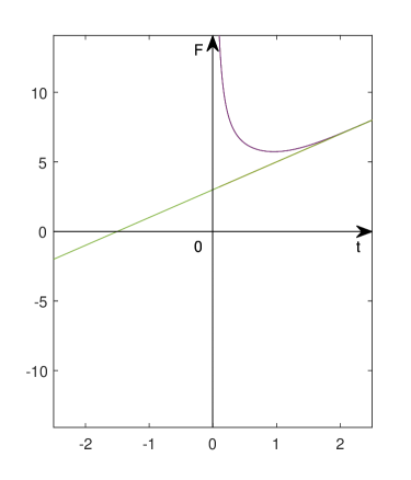
This means that any function in the family cannot be fitted by any generic Hölder potential on any shift space of finite type globally, considering Theorem 4.1. In the following we deny the possibility that they can be fitted by non-generic Hölder potentials on shift spaces of finite type.
4.3 Definition.
A continuous potential on a shift space of finite type is said to be non-generic if for some normalised potential , the spectral radius of the complex Ruelle operator equals for some .
One can show that if is non-generic then there exists a continuous function , and a locally constant potential , such that
| (4.2) |
4.4 Proposition.
For any and any with , there does not exist any non-generic Hölder potential on any shift space of finite type such that
on .
Proof.
Note that for a non-generic Hölder potential on a shift space of finite type, according to (4.2), we have
,
in which is some locally constant potential. By the explicit formula (see Lemma 5.3) for the pressure functions of locally constant potentials on shift spaces of finite type, we see that any cannot be fitted by pressure of any non-generic Hölder potential globally. ∎
5. Local fitting of analytic germs via pressures of locally constant potentials
In this section we deal with the local fitting of analytic functions by the pressures of Hölder potentials, especially the pressures of piecewise constant ones. Firstly we borrow some notion originating from analytic continuation.
5.1 Definition.
A germ at is the sum of infinite power series
for some .
The convergent radius (the superior of values on the germ converges) of the power series is called the radius of the germ. We are only interested in germs of radius . The following problem will be our concern in this section.
5.2 Problem.
For a germ
at with some strictly positive radius, does there exist some Hölder potential on some shift space of finite type and some , such that
on ?
The question can still be understood in Katok’s flexibility program in the class of symbolic dynamical systems, or even in some smooth systems. Obvious conditions to guarantee a positive answer to the problem are (1.5) and
| (5.1) |
Condition (5.1) guarantees convexity of the germ (in some neighbourhood of ) while (1.5) guarantees the supporting lines of the germ intersect the vertical axis in a bounded set in (also in some neighbourhood of ). We are especially interested in its answer when the Hölder potential in Problem 5.2 is required to be a piecewise constant one. We have seen the importance of the family of locally constant potentials in approximating convex analytic functions in Corollary 1.4. In fact Corollary 1.4 has some interesting interpretation in approximation theory [Tim], when we consider the explicit expressions of the pressures of locally constant potentials on the shift space of finite type. For , recall that
.
5.3 Lemma.
For an integer , consider some locally constant potential
for on the shift space , we have
for any .
Proof.
5.4 Remark.
The result can be extended to transitive subshifts of finite type. In this case the pressure is the logarithm of the maximal eigenvalue of some appropriate matrix.
5.5 Corollary.
Let be a convex Lipschitz function on for some , such that its supporting lines intersect the vertical axis in with . Then there exists some and some sequences of constants
,
such that
| (5.2) |
for any .
Proof.
Take for the symbolic set in the proof of Corollary 1.4, then the locally constant potential admits constant values respectively on corresponding level- cylinder sets. Denote these values by for . According to Lemma 5.3,
∎
Corollary 5.5 indicates that logarithm of the finite sums of the exponential maps in the family are dense in the space of certain convex Lipschitz maps on . The above approximation is uniform with respect to in a bounded set. This makes the family (family of locally constant potentials) important in detecting the properties of certain convex Lipschitz maps (among continuous or Hölder potentials).
From now on we turn our attention to Problem 5.2, but with restriction on locally constant potentials. We focus on locally constant potentials defined on the level- cylinder sets, whose theory is presumably parallel to the ones defined on the deeper cylinder sets. On the shift space with , consider the locally constant potential
for , in which are all constants. Let
,
so
by Lemma 5.3. Let
and
.
Through some elementary calculations one can check that
while
| (5.3) |
Let
,
one can check that
.
In the following we will often fix , so we will frequently write
with omitted for convenience. Similar notations apply to other terms above. Let
| (5.4) |
| (5.5) |
be two equations with unknowns for fixed and some . Let
and
.
They are both dimensional smooth hypersurfaces. We first present readers with the following result on fitting an analytic function
with subject to (1.5) around some fixed by pressures of locally constant potentials on general shift spaces of finite type.
5.6 Theorem.
Let satisfying (1.5) and
| (5.6) |
Then there exists some and some sequence , such that the locally constant potential
for on the full shift space satisfies
on .
Proof.
In fact it suffices for us to show that the system of equations
with unknowns admits a solution under conditions of the theorem. Without loss of generality we assume
| (5.7) |
Under this assumption, it is easy to see that
.
Now we estimate the values of with approaching the terminals. When approaches the right terminal from below, we have
in virtue of (1.5). When approaches the left terminal from above, we have
in virtue of (5.6). Since is a smooth hypersurface, by the mean value theorem, there exists some satisfying (5.4) and (5.5) simultaneously. At last, for on the full shift space , let
be the locally constant potential. As is analytic, there exists some such that
for . ∎
5.7 Remark.
The core step in the proof of Theorem 5.6 is in fact finding the extremes of the function subject to (5.4), (1.5) and (5.6). One can detect the points of extremes by the Karush-Kuhn-Tucker (KKT) conditions [Kar, KT], which generalizes the method of Lagrange multipliers by allowing inequality subjections.
Be careful that those all depend on in fact. Theorem 5.6 induces the following interesting flexibility result on fitting certain analytic functions locally by pressures of locally constant potentials on general shift space of finite type.
5.8 Corollary.
Let and satisfy (1.5). Then there exists some , such that for any , there exist some some and some sequence , such that the locally constant potential
for on the full shift space satisfies
on .
Proof.
Note that on some particular symbolic spaces Theorem 5.6 and 5.8 may be trivial. For example, for given without any subjections, by choosing , consider the constant potential
on the -shift space with symbols . It is easy to see that
on . However, our results guarantee conclusions on general shift spaces.
From now on we go towards the proof of Theorem 1.8. For fixed and , let
.
We describe some topological properties of the set in the following result.
5.9 Lemma.
For fixed subject to (1.5) and , in case and , it is a compact -dimension smooth manifold.
Proof.
The Jacobian of the functions and with respect to is
Its rank is strictly less than if and only if
.
Since , this is excluded from points in . By the implicit function theorem [Lan], if is not empty, it is an -dimension smooth manifold locally. The gradient of the function is
,
whose individual components will always be strictly positive. The gradient of the function is
,
with the -th individual component vanishes if and only if for . So and cannot be tangent to each other. Moreover, note that
if while
if for any . These force the intersection of zeros of the two functions and to be connected, if the intersection is not empty. This implies is a manifold globally in case of being nonempty. is compact since it is a bounded set. ∎
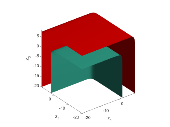
Let
and
be the corresponding surfaces with . Figure 2 depicts parts of the two -dimension surfaces, whose intersection will be a -dimension smooth curve.
Equipped with all the above results, now we are ready to prove Theorem 1.8.
Proof of Theorem 1.8.
First, for the given and satisfying (1.5), if is large enough, is not empty according to Corollary 5.8. So is a compact -dimension smooth manifold for large enough. In the following we always assume is large enough. Now let
while
| (5.8) |
For any , since is a smooth manifold, there exist , such that satisfies and
| (5.9) |
simultaneously. Now let
for on the full shift space . It is a locally constant potential. According to (5.3) and (5.9), we have
| (5.10) |
Since satisfies and , we have
| (5.11) |
while
| (5.12) |
Note that is analytic with respect to on for any , so there exists some , such that (1.6) holds on , considering (5.10), (5.11) and (5.12). ∎
In the following we illustrate some dependent relationship between
and some particular satisfying (1.5). There should be some universal relationship between them, while we hope the following observations will provide some hints. The first one is that it is possible for for some .
5.10 Proposition.
Let and satisfy (1.5). Then for if and only if
| (5.13) |
Proof.
This result does not tell things about the sequence
for given , since (5.13) will never be true for any large enough for fixed . The following result describes some limit behaviour of the sequence
for .
5.11 Proposition.
Let , in symbols of Theorem 1.8, we have
| (5.14) |
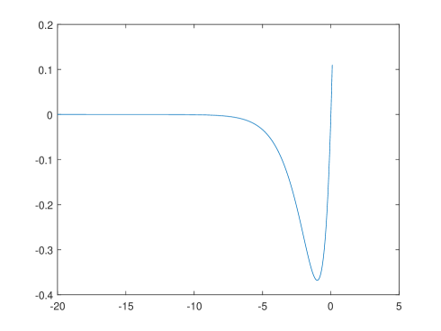
To justify Proposition 5.11, we first illustrate some basic properties about the function for .
5.12 Lemma.
For , is strictly decreasing on , strictly increasing on , while it attains its minimum at . It admits one and only one inflection in .
Proof.
One can check these conclusions by some direct computations on the first and second derivatives of the function . ∎
In Figure 3 we depict the graph of .
Proof of Proposition 5.11.
Since we are considering the limit behaviour of , we always assume is large enough throughout the proof. Now consider the following two equations
| (5.15) |
and
| (5.16) |
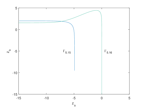
with unknowns . Let
and
.
We describe the graph of and separately in the following. is a dimensional smooth curve with two asymptotes and . It is strictly decreasing when we consider the curve as the graph of the function
for . is also a dimensional smooth curve with two asymptotes and . When we consider the as the graph of the function
as the implicit function induced by , it is strictly increasing for , strictly decreasing for , with its maximum attained at . Let be the smaller one of the two intersections of and , then and must intersection at some unique point . Obviously
since . Now we analyse the order of with respect to as . Let
.
One can check that
while
.
These imply that
.
Note that for . Now
from which it is easy to see that
.
This forces
,
considering (5.8).
∎
We provide the readers with the curves and in Figure 4. Obviously some more general conclusions are available if one considers variations of the parameters in Proposition 5.11. At last we provide the readers with some solutions and in Table 3, from which one can see the order of decay and increase of the sequences with respect to clearly.
| -1.8599539391797653780996686364493 | 1.7634042477581860636342812520981 | |
| -4.6278529940301947157458180305676 | 1.8580906928560505140960875180438 | |
| -7.2278923365046354303919671475052 | 1.8965708210067454817129699066334 | |
| -9.7529279223041958189401940128674 | 1.9180710389285259082138396366755 | |
| -12.23426184122178540565187685582 | 1.9319494203818796717151866525306 | |
| -14.686689485112383196253350885528 | 1.941701042038176132682488585943 | |
| -17.118475509130338419321449219176 | 1.9489507180131363431129601417792 | |
| -19.534737736752111249670741176574 | 1.9545628133690736391913141129777 | |
| -21.938877884281897893422087428599 | 1.9590417833080193886068703580662 | |
| -24.333277592346602338263750350022 | 1.9627027620469153955488959845337 | |
| -26.719672172461371813735932628894 | 1.9657531814729595378854181456218 | |
| -29.099366670257435261982274861811 | 1.9683353707111573738492465130807 | |
| -31.473368167571030624456199153849 | 1.970550350496947761285545176838 | |
| -33.842470627269595326611535858951 | 1.9724718685216929582206115029034 | |
| -36.20731141238751139407393422892 | 1.9741550583546827046855344007126 | |
| -38.568410155198951836337896822881 | 1.97564198636943790477268372057 | |
| -40.926196222869058989174011616314 | 1.9769653208730088904749619599928 | |
| -43.28102858421294787781225809291 | 1.9781508271703613365389080750692 | |
| -45.633210475623427729647938869856 | 1.9792191056459012534062976747755 | |
| -47.983000423353389741328990557576 | 1.9801868284846851379610473178804 | |
| -50.330620660008332271820694306839 | 1.9810676363715292020369862557429 | |
| -52.676263643082855194671803053742 | 1.9818727996772032079642260800619 | |
| -55.020097168291592849066888176454 | 1.9826117134133018944596936081392 | |
| -57.362268427077060922578379063246 | 1.9832922728467949817312209115653 | |
| -59.702907260160132201351723856461 | 1.9839211621102961084222105523408 | |
| -62.042128791447074538616865826092 | 1.9845040784885601043186175801529 | |
| -64.380035579030470553978577616248 | 1.9850459085371711281404342988732 | |
| -66.716719386002755126963619613768 | 1.9855508677057357884921072471682 | |
| -69.052262649137714881922574449762 | 1.9860226120088820356292880321385 | |
| -71.386739705385277326962820249044 | 1.9864643280735340181774784668139 | |
| -73.7202178226698188293210417966 | 1.9868788063025456510398996161088 | |
| -76.052758071376257724956806229201 | 1.9872685007417625212636588061233 | |
| -78.384416065240707497606345034329 | 1.9876355783911370649894789906831 | |
| -80.715242594490126828808238297291 | 1.9879819600725889180558042388717 | |
| -83.045284169538297201269228695051 | 1.9883093544968926933418986392956 | |
| -85.374583490011093204926910773042 | 1.9886192868162322855194994642595 | |
| -87.703179851099500408441885242821 | 1.9889131226778662869710690898493 | |
| -90.031109497045012553979249690171 | 1.9891920885858755212588911444123 | |
| -92.358405929815521230622254914238 | 1.9894572892164831961499157326311 | |
| -94.685100179630439886817678169988 | 1.9897097222064583485549741614556 |
References
- [BDL] V. Baladi, M. Demers and C. Liverani, Exponential Decay of Correlations for Finite Horizon Sinai Billiard Flows, Inventiones mathematicae, volume 211, pp. 39-177 (2018).
- [BKR] J. Bochi, A. Katok and F. Rodriguez Hertz, Flexibility of Lyapunov exponents, Ergod. Theory Dyn. Syst., 42(2): Anatole Katok Memorial Issue Part 1: Special Issue of Ergodic Theory and Dynamical Systems, February 2022, pp. 554-591.
- [Bow] R. Bowen, Equilibrium States and the Ergodic Theory of Anosov Diffeomorphisms, Lecture Notes in Mathematics 470, Springer, 1975.
- [CP] Z. Coelho and W. Parry, Central Limit asymptotics for shifts of finite type, Israel J. Math., Vol 69, N.2, (1990).
- [Fel] W. Feller, An Introduction to Probability Theory and its Applications, Vol. 2, 2nd ed., John Wiley & Sons, New York, 1971.
- [GLP] P. Giulietti, C. Liverani and M. Pollicott, Anosov Flows and Dynamical Zeta Functions, Annals of Mathematics, 178, 2 (2013) 687-773.
- [GT] D. Gilbarg and N. Trudinger, Elliptic Partial Differential Equations of Second Order, New York: Springer, 1983.
- [IRV] G. Iommi, F. Riquelme and A. Velozo, Entropy in the cusp and phase transitions for geodesic flows, Isr. J. Math., 225 (2018) 609-659.
- [IT1] G. Iommi and M. Todd, Transience in dynamical systems, Ergod. Theory Dyn. Syst., 33(5) (2013) 1450-1476.
- [IT2] G. Iommi and M. Todd, Differentiability of the pressure in non-compact spaces, arXiv:2010.10250 [math.DS], 2020.
- [Kar] W. Karush, Minima of Functions of Several Variables with Inequalities as Side Constraints (M.Sc. thesis), Dept. of Mathematics, Univ. of Chicago, 1939.
- [KS1] M. Kotani and T. Sunada, The pressure and higher correlations for an Anosov diffeomorphism, Ergod. Theory Dyn. Syst., 21 (2001), no. 3, 807-821.
- [KS2] M. Kotani and T. Sunada, A Central Limit Theorem for the Simple Random Walk on a Crystal Lattice, Proceedings of the Second ISAAC Congress, pp 1-6, 2000.
- [KQ] T. Kucherenko and A. Quas, Flexibility of the Pressure Function, Comm. Math. Phys., to appear.
- [KQW] T. Kucherenko, A. Quas and C. Wolf, Multiple phase transitions on compact symbolic systems, Adv. in Math., 385 (2021).
- [KT] H. Kuhn and A. Tucker, Nonlinear programming, Proceedings of 2nd Berkeley Symposium, Berkeley: University of California Press, pp. 481-492, 1951.
- [Lal] S. Lalley, Ruelle’s Perron-Frobenius theorem and central limit theorem for additive functionals of one-dimensional Gibbs states, Proc. Conf. in honour of H. Robbins, 1985.
- [Lan] S. Lang, Fundamentals of Differential Geometry, Graduate Texts in Mathematics 191, New York: Springer, 1999.
- [Lop1] A. Lopes, The Dimension spectrum and a mathematical model for phase transition, Adv. in Appl. Math., 11 No. 4 (1990), 475-502.
- [Lop2] A. Lopes, The first order level 2 phase transition in thermodynamic formalism, J. Sta. Phys., 60 Nos 3/4 (1990), 395-411.
- [Lop3] A. Lopes, The Zeta Function, non-differentiability of the pressure, and the critical exponent of transition, Adv. in Math., 101 (1993), 133-165.
- [PP] W. Parry and M. Pollicott, Zeta functions and the periodic orbit structure of hyperbolic dynamics, Astérisque, Vol. 187-188, 1990.
- [Rou] J. Rousseau-Egèle, Un théorèdme de la limite locale pour une classe de transformations dilatantes et monotones par morceaux, Ann. of Prob., 11 (1983), 772-788.
- [Rue1] D. Ruelle, Thermodynamic formalism: The mathematical structures of equilibrium statistical mechanics, Second edition, Cambridge University Press, Cambridge, 2004.
- [Rue2] D. Ruelle, Statistical mechanics of a one-dimensional lattice gas, Comm. Math. Phys., 9 (1968), 267-278.
- [Sar] O. Sarig, On an example with a non-analytic topological pressure, C. R. Acad. Sci. Paris, Sér. I Math., 330 (2000) 311-315.
- [Tim] A. Timan, Theory of Approximation of Functions of a Real Variable, translated by J. Berry from ’Teoriya priblizheniya funktsii deistvitel’nogo peremennogo’, Pergamon Press LTD., 1963.
- [Wal1] P. Walters, An introduction to ergodic theory, Graduate Texts in Mathematics 79, Springer, 1981.
- [Wal2] P. Walters, A necessary and sufficient condition for a two-sided continuous function to be cohomologous to a one-sided continuous function, Dyn. Syst., 18(2) (2003) 131-138.