Riemannian conditional gradient methods for composite optimization problems
Abstract
In this paper, we propose Riemannian conditional gradient methods for minimizing composite functions, i.e., those that can be expressed as the sum of a smooth function and a geodesically convex one. We analyze the convergence of the proposed algorithms, utilizing three types of step-size strategies: adaptive, diminishing, and those based on the Armijo condition. We establish the convergence rate of for the adaptive and diminishing step sizes, where denotes the number of iterations. Additionally, we derive an iteration complexity of for the Armijo step-size strategy to achieve -optimality, where is the optimality tolerance. Finally, the effectiveness of our algorithms is validated through some numerical experiments performed on the sphere and Stiefel manifolds.
keywords:
Conditional gradient methods, Riemannian manifolds, composite optimization problems , Frank-Wolfe methods[label1]organization=Graduate School of Informatics, Kyoto University, country=Japan
1 Introduction
The conditional gradient (CG) method, also known as the Frank-Wolfe algorithm, is a first-order iterative method, widely used for solving constrained nonlinear optimization problems. Developed by Frank and Wolfe in 1956 [1], the CG method addresses the problem of minimizing a convex function over a convex constraint set, particularly when the constraint set is difficult, in the sense that the projection onto it is computationally demanding.
The convergence rate of , where denotes the number of iterations, for the conditional gradient method has been presented in several studies [2, 3]. Recent advancements in the field have focused on accelerating the method [4, 5]. The versatility of this method is also clear, since many applications can be found in the literature (see, for instance, [6, 7]). Furthermore, the CG method has recently been extended to multiobjective optimization [8, 9, 10].
Meanwhile, composite optimization problems, where the objective function can be decomposed into the sum of two functions, have become increasingly important in modern optimization theory and applications. Specifically, the objectives of these problems take the form , where is a smooth function and is a possibly non-smooth and convex function. This structure arises naturally in many areas, including machine learning and signal processing, where often represents a data fidelity term and serves as a regularization term to promote desired properties such as sparsity or low rank [11, 12, 13].
To deal with such problems efficiently, various methods have been developed. Classical approaches include proximal gradient methods [14, 15, 16], which address the non-smooth term using proximal operators, and accelerated variants such as FISTA [17]. Other methods, such as the alternating direction method of multipliers (ADMM) [18], decompose the problem further to enable parallel and distributed computation. For problems with specific structures or manifold constraints, methods like the Riemannian proximal gradient have been proposed in [19, 20], extending proximal techniques to non-Euclidean settings. Recently, the CG method in Riemannian manifolds has been proposed in [21], and the CG method for composite functions, called the generalized conditional gradient (GCG) method, has also been discussed in many works [9, 22, 23, 24].
In this paper, we propose GCG methods on Riemannian manifolds, with general retractions and vector transport. We also focus on three types of step-size strategies: adaptive, diminishing, and those based on the Armijo condition. We provide a detailed discussion on the implementation of subproblem solutions for each strategy. For each step-size approach, we analyze the convergence of the method. Specifically, for the adaptive and diminishing step-size strategies, we establish a convergence rate of , where represents the number of iterations. For the Armijo step size strategy, we derive an iteration complexity of , where represents the desired accuracy in the optimality condition.
This paper is organized as follows. In Section 2, we review fundamental concepts and results related to Riemannian optimization. In Section 3, we introduce the generalized conditional gradient method on Riemannian manifolds with three different types of step size. Section 4 presents the convergence analysis, while Section 5 focuses on the discussion of the subproblem. Section 6 explores the accelerated version of the proposed method. Numerical experiments are presented in Section 7 to demonstrate the effectiveness of our approach. Finally, in Section 8, we conclude the paper and suggest potential directions for future research.
2 Preliminaries
This section summarizes essential definitions, results, and concepts fundamental to Riemannian optimization [25]. The transpose of a matrix is denoted by , and the identity matrix with dimension is written as . A Riemannian manifold is a smooth manifold equipped with a Riemannian metric, which is a smoothly varying inner product , defined on the tangent space at each point , where and are tangent vectors in the tangent space . The tangent space at a point on the manifold is denoted by , while the tangent bundle of is denoted as . The norm of a tangent vector is defined by . When the norm and the inner product are written as and , without the subscript, then they are the Euclidean ones. For a map between two manifolds and , the derivative of at a point , denoted by , is a linear map that maps tangent vectors from the tangent space of at to the tangent space of at . The Riemannian gradient of a smooth function at a point is defined as the unique tangent vector at that satisfies the equation for every tangent vector . We also define the Whitney sum of the tangent bundle as .
In Riemannian optimization, a retraction is employed to map points from the tangent space of a manifold back onto the manifold.
Definition 2.1.
[25] A smooth map is called a retraction on a smooth manifold if the restriction of to the tangent space at any point , denoted by , satisfies the following conditions:
-
1.
,
-
2.
for all ,
where and are the zero vector of and the identity map in , respectively.
Depending on the problem and the specific properties of the manifold, different types of retractions can be utilized. Many Riemannian optimization algorithms employ a retraction that generalizes the exponential map on . For instance, assume that we have an iterative method generating iterates . In Euclidean spaces, the update takes the form , while in the Riemannian case it is generalized as
where is a descent direction and is a step size.
Another essential concept is the vector transport, which is critical in Riemannian optimization to maintain the intrinsic geometry of the manifold during computations.
Definition 2.2.
[25] A map is called a vector transport on if it satisfies the following conditions:
-
1.
There exists a retraction on such that for all and .
-
2.
For any and holds, where is the zero vector in , i.e., is the identity map in .
-
3.
For any , and holds, i.e., is a linear map from to .
The adjoint operator of a vector transport , denoted by , is a vector transport satisfying:
where . The inverse operator of a vector transport, denoted by , is a vector transport satisfying:
where id is the identity operator.
Note that a map defined by is also a vector transport, where is the parallel transport along the geodesic connecting and with the exponential map Exp as a retraction. Parallel transport is a specific case of vector transport that preserves the length and angle of vectors as they are transported along geodesics, thereby preserving the intrinsic Riemannian metric of the manifold exactly. In contrast, vector transport is a more general operation that allows for the movement of vectors between tangent spaces in a way that approximately preserves geometric properties, and it may not necessarily follow geodesics or maintain exact parallelism. If there is a unique geodesic between any two points in , then the exponential map has an inverse . This geodesic represents the unique shortest path and the geodesic distance between and in is given by .
Now, we define geodesic convexity sets and functions, -smoothness, and related concepts on Riemannian manifolds as follows:
Definition 2.3.
A set is called geodesically convex if for any , there is a geodesic with and for all .
Definition 2.4.
A function is called geodesically convex, if for any , we have for any , where is the geodesic connecting and .
Proposition 2.1.
[21] Let be a smooth and geodesically convex function. Then, for any , we have
Considering the definition of geodesic convexity and defining the retraction through , we can easily obtain the following result.
Proposition 2.2.
Let be a smooth and geodesically convex function. Then, for any and , we have
Definition 2.5.
A function is called geodesically -smooth or with -Lipschitz continuous gradient if there exists such that
| (1) |
where is the geodesic distance between and and is the vector transport from to . It is equivalent to
A similar concept is defined below.
Definition 2.6.
[20] A function is called -retraction-smooth with respect to a retraction in if for any and any such that , we have
| (2) |
3 Riemannian generalized conditional gradient method
In this paper, we consider the following Riemannian optimization problem:
| (3) | ||||
| s.t. |
where is a compact geodesically convex set and is a composite function with being continuously differentiable and being a closed, geodesically convex and lower semicontinuous (possibly nonsmooth) function. Here, we can also consider as an extended-valued function. All the analyses would still apply, but we omit the infinity for simplicity. Also, we make the following assumption.
Assumption 1.
The set is a geodesically convex and complete set where the retraction and its inverse are well-defined and smooth over . Additionally, the inverse retraction is continuous with respect to both and .
As discussed in [26, Section 10.2], for general retractions, over some domain of which contains all pairs , the map can be defined smoothly jointly in and . In this sense, we can say that the above assumption is reasonable.
Now, let us recall the CG method in the Euclidean space. Consider minimizing a convex function over a convex compact set . At each iteration , the method solves a linear approximation of the original problem by finding a direction that minimizes the linearized objective function over the constraint set , i.e., Then, it updates the current point using a step size along the direction , i.e., For composite functions of the form , where is smooth and is convex, the CG method can be adapted to handle the non-smooth term . The update step becomes:
In this case, is the new objective function for the subproblem, which remains convex due to the convexity of , compacity of and the linearity of . The convexity of ensures that this subproblem also has a solution. The step size can be chosen using various strategies. The CG method is particularly useful when the constraint set is not an easy set, making projection-based methods computationally expensive.
The exponential map, the parallel transport, and specific step size are used in the Riemannian CG method proposed in [21]. Now we extend this approach to a more general framework for composite optimization problems, without specifying the retraction and the vector transport.
Step 0. Initialization:
Choose and initialize .
Step 1. Compute the search direction:
Compute an optimal solution and the optimal value as
| (4) |
| (5) |
Define the search direction by .
Step 2. Compute the step size:
Compute the step size .
Step 3. Update the iterates:
Update the current iterate
Step 4. Convergence check:
If a convergence criteria is met, stop; otherwise, set and return to Step 1.
Our method is presented in Algorithm 1. In Step 1, we need to solve the subproblem (4), which, similarly to the Euclidean case, is related to the linear approximation of the objective functions. In Step 2, we compute the step size based on some strategies that we will mention later. In Step 3, we update the iterate by using some retraction. Note that if in (4), then , which implies that . And since , the subproblem is equivalent to
| (6) |
In the subsequent sections, we will examine the convergence properties of the sequence generated by the Algorithm 1, specifically focusing on three distinct and rigorously defined strategies for step size determination, which is also discussed in [8], as elaborated below.
Armijo step size: Let and . The step size is chosen according to the following line search algorithm:
Step 0. Set and initialize .
Step 1. If
then set and return to the main algorithm.
Step 2. Find , set , and go to Step 1.
Adaptive step size: For all , set
Diminishing step size: For all , set
4 Convergence analysis
In this section, we will provide the convergence analysis for three types of step sizes. The following assumption will be used in the convergence results.
Assumption 2.
The function is geodesically -smooth, namely, there exist a constant such that (1) holds.
Since is a compact set, we can assume without loss of generality that is a compact set, its diameter is finite and can be defined by
| (7) |
Lemma 4.1.
Let with and , where and represents the geodesic joining with . Then, we have
| (8) |
Proof.
From the definition of , we have
where the first inequality comes from the -smoothness of and the second inequality is due to the geodesic convexity of . Then, from the definition of in (5), and using the fact that , we obtain the desired result. ∎
Additionally, we can derive the following proposition.
Proposition 4.2.
Proof.
From Lemma 4.1, we obtain
Define . Then, we get
From the convexity of , we have
Then we have , which gives
Now, let us expand and gradually express in terms of . Ultimately, for the recursive relation at step , we obtain:
that is,
Rearranging the terms completes the proof. ∎
Now we present a result associated to general sequences of real numbers, which will be useful for our study of convergence and iteration complexity bounds for the CG method.
Lemma 4.3.
[14, Lemma 13.13] Let and be nonnegative sequences of real numbers satisfying
where and is a positive number. Suppose that for all . Then
-
(i)
for all
-
(ii)
for all where .
4.1 Analysis with the adaptive and the diminishing step sizes
Theorem 4.4.
Proof.
From Lemma 4.1 and the diminishing step size , we have
| (10) |
Considering the adaptive step size , we have , so the inequality (10) still holds.
The above theorem also indicates that the iteration complexity of the method is . Note that a similar result can be obtained by following the proof of [22, Corollary 5].
4.2 Analysis with the Armijo step size
In the following lemma, we prove that there exist intervals of step sizes satisfying the Armijo condition.
Lemma 4.5.
Let , and . Then, there exists such that
| (11) |
Proof.
In the subsequent results, we assume that the sequence generated by Algorithm 1 is infinite, which means that for all .
Assumption 3.
Set . All monotonically nonincreasing sequences in are bounded from below.
Theorem 4.6.
Proof.
(1) By the Armijo step size, the fact that for all , and by Lemma 4.5, we have
| (12) |
which implies that the sequence is monotonically decreasing. On the other hand, since and is compact, there exists that is a accumulation point of a subsequence of . Without loss of generality, assume that .
From (12), with for some , we have , where exists from Assumption 3. Taking , we have . Therefore, we have . If
| (13) |
then the assertion holds. So we consider the case
| (14) |
Assume that for some . Suppose by contradiction that . Then, there exist and such that
Without loss of generality, we assume that there exists such that
Since for all , by Armijo step size, there exists such that
Then, we have
| (15) |
On the other hand, since , and is geodesically convex, then
namely,
| (16) |
Since is differentiable and , for all , we have
| (17) |
which, together with (16) and (17) and the definition of , gives
| (18) | ||||
Combining (18) with (15), we obtain for all ,
that is,
Then, we have
On the other hand, from the fact that and (18), we obtain
Combining the two results above, it holds that
Since as , we obtain , which contradicts the fact that . Thus, .
(2) Let be an accumulation point of the sequence . Assume that is not a stationary point of , namely . By the definition of in (5), we have
and by taking the limit we obtain
since is continuously differentiable, is lower semicontinuous and Assumption 1 holds. Now taking the minimum over and because is not stationary point of ,
which contradicts to , so is a stationary point of .
Also, due to the monotonicity of the sequence given in (12), we obtain , which completes the proof. ∎
The following theorem provides the iteration complexity of Algorithm 1 with Armijo step size, indicating that after a finite number of steps, the iteration complexity of the method could be .
Theorem 4.7.
Proof.
First, we consider that . From the Armijo step size, we can say that there exists such that
Recall that from Lemma 4.1, we have
Combining the above two inequalities, we conclude that:
namely,
Defining , we get
| (19) |
From Theorem 4.6, we have . Then, without loss of generality, for sufficiently large , when , . Then (19) still holds for . Taking it into (12), we obtain
| (20) |
Namely (20) holds for all . By summing both sides of the second inequality in (20) for , we obtain
where is an accumulation point of , as in Theorem 4.6.
This implies . Namely, Algorithm 1 returns satisfying in at most iterations. ∎
Furthermore, we can obtain stronger results by making additional assumptions about the objective function .
Assumption 4.
Assume the function is Lipschitz continuous with constant in , namely, . And for generated by Algorithm 1, there exists such that .
As tends to infinity, we can assume without loss of generality that lies within a compact neighborhood of . Due to the smoothness of the inverse retraction, this ensures that remains bounded. Hence, Assumption 4 is reasonable. Moreover, we define
| (21) | ||||
Then we present the following lemma, which is crucial for the subsequent convergence rate analysis.
Lemma 4.8.
Proof.
Theorem 4.9.
Proof.
By the Armijo step size and the fact that for all , and Lemma 4.5, we have
| (22) |
which implies that the sequence is monotone decreasing. Combined with Lemma 4.8, we have
| (23) |
On the other hand, since and is compact, there exists a limit point of . Let be a subsequence of such that . Since and is Lipschitz continuous, we have
for all . Considering that is continuous and , we conclude from the last inequality that . Thus, due to the monotonicity of the sequence , we obtain that . Therefore, from (23), , which implies item (i).
Therefore, satisfies in at most iterations. ∎
5 Solving the subproblem
In this section, we will propose an algorithm for solving the subproblem of the RGCG method. Recall that in Algorithm 1, given the current iterate , we need to compute an optimal solution and the optimal value as
| (24) |
| (25) |
Now define as the descent direction on the tangent space, i.e.,
| (26) |
We also define
| (27) |
We observe that for both (24) and (26), the retraction is not necessarily a convex function, which implies that the resulting optimization problem is not necessarily convex. Non-convex problems are inherently more challenging to solve. To address this, we aim to transform the subproblem into a series of convex problems, which is similar to the general method for solving Riemannian proximal mappings proposed in [20].To ensure that we can locally approximate and simulate the subproblems effectively, we consider the following assumption:
Assumption 5.
The manifold is an embedded submanifold of or is a quotient manifold whose total space is an embedded submanifold of .
Let us now present a way to find the approximation of . Assume that , and let denote the current estimate of . Observe that
for any . Let and . Since the retraction is smooth by definition, we obtain , where means . Then, we obtain:
where the second equality comes from the Lipschitz continuity of (see Assumption 4). Note that the middle parts of the above term
| (28) |
can be interpreted as a simple local model of . Thus, to obtain a new estimate from , we first compute a search direction by minimizing (28) on , and then update along the direction , as described in Algorithm 2.
It is easy to find that Algorithm 2 is the application of the Riemannian GCG method for problem (26) with a proper retraction. Moreover, note that (29) can be solved by the subgradient method or proximal gradient method.
Require: An initial iterate ; a small positive constant ;
1: for , do
2:
3: Compute by solving
| (29) |
4:
5: while do
6: ;
7: end while
8: ;
4: end for
6 Accelerated conditional gradient methods
Now we consider the accelerated version of the RCG method. We noticed that based on the accelerated gradient methods, Li et al. [4] establish links between subproblems of conditional gradient methods and the notion of momentum. They proposed a momentum variant of CG method and proved that it converges with a fast rate of . However, the extension of this work to the Riemannian manifold case is not trivial, even though there are works on Nesterov accelerated methods on Riemannian manifolds [27]. Based on these existing works, here we propose an accelerated CG method on Riemannian manifolds for composite function.
Step 0. Initialization Choose , and initialize , .
Step 1.
Step 2. Compute an optimal solution and the optimal value as
Step 3. Stopping criteria If , then stop.
Step 4. Compute the iterate Set
Step 5. Beginning a new iteration Set and go to Step 1.
Analyzing the convergence and convergence rate for the above accelerated method is challenging, primarily due to the inherent nonconvexity of the problem and the complexities introduced by transporting tangent vectors. A comprehensive analysis of the accelerated method is beyond the scope of this paper. However, the performance of the accelerated method compared to the non-accelerated method is shown in the numerical experiments in Section 7.
7 Numerical experiments
Sparse principal component analysis (Sparse PCA) plays a crucial role in high-dimensional data analysis by enhancing the interpretability and efficiency of dimensionality reduction. Unlike traditional PCA, which often produces complex results in high-dimensional settings, Sparse PCA introduces sparsity to refine data representation and improve clarity. This is particularly relevant in fields such as bioinformatics, image processing, and signal analysis, where interpretability and reconstruction accuracy are essential. In this section, we consider Sparce PCA problems to check the validity of our proposed methods. We explore two models for sparse PCA as in [20], where we set in each problem.
7.1 Sparse PCA on the sphere manifold
Now consider problems in sphere manifolds The specific optimization problem is formulated as follows:
| (30) |
where denotes the -norm, and is a parameter. Here, we use the exponential mapping as the retraction, i.e.,
The inverse exponential mapping can also be computed by applying the inverse exponential mapping on the unit sphere [20], i.e.,
We now need to introduce an important result as below.
Lemma 7.1.
[20, Lemma D.1] For any and , the minimizer of the optimization problem
is given by
where is the index of the largest magnitude entry of (break ties arbitrarily), denotes the -th column in the canonical basis of , and is defined by
The subproblem (4) applied to (30), can be written as
| (31) |
Let us not check how to compute its solution. Let , and let denote the current estimate of the minimizer of over the unit sphere. The next estimate, , is obtained by solving the following optimization problem:
which is equal to
In other words, is approximated by its first-order Taylor expansion around at each iteration. To solve the above problem, note that since for all , the problem is further equivalent to:
| (32) |
The above problem can be actually solved using Lemma 7.1.
7.2 Sparse PCA on the Stiefel manifold
Now consider sparse PCA on the Stiefel manifold. The specific optimization problem is formulated as follows:
| (33) |
where denotes the Stiefel manifold, and . Moreover, the term aims to maximize the variance of the data, characterizes the sparsity of the principal components, and is the original data matrix. The tangent space is defined as
Here we use the Euclidean metric as the Riemannian metric. We also use the polar decomposition as the retraction, i.e.,
The vector transport by differentiated retraction is given in [28, Lemma 10.2.1] by
where and is the solution of the Sylvester equation
For ease of notation, we define the operator by and rewrite the subproblem (29) as
| s.t. |
This can be solved by the subgradient method or the proximal gradient method. For the subgradient method, note that the subgradient of can be calculate through function , which is defined as:
-
1.
if ,
-
2.
if ,
-
3.
if ,
where is the element of . Then the subgradient of the above problem can be written as
7.3 Numerical results
We implemented the algorithms in Python 3.9.12, and the experiments were carried out on a MacBook Pro with an Apple M1 Pro chip and 16GB of RAM.
7.3.1 Sphere experiment
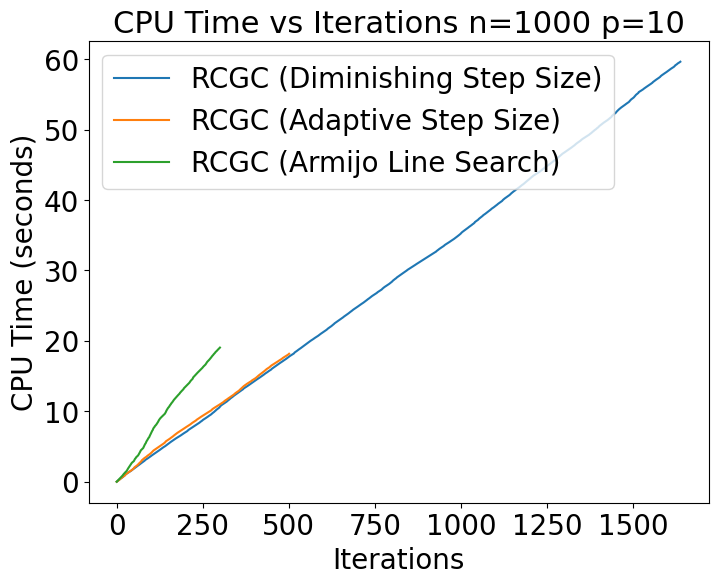
For the example (30), we conducted experiments on a -dimensional problem, using a randomly generated standardized and a regularization parameter . The experiment evaluates Armijo step size with parameters , , and . Each experiment runs for the same original problem 10 times with different initial points and stops if the norm of is less than or if the difference between the latest function value and the function value from five iterations ago is less than . In this example, our experiments were conducted on high-dimensional spheres, with dimensions set to 10, 100, and 1000, across ten runs for each method. In the numerical experiments, we observed that solving the subproblems typically converges after just one iteration, suggesting that the local model provides an effective approximation of the original subproblem.
As shown in Table 1 and Figure 1, the results demonstrated that the Armijo step-size strategy consistently outperformed the others in terms of computational time and required iterations to achieve function value convergence. Overall, our findings suggest that the Armijo step-size strategy offers significant advantages in efficiency and speed, particularly in high-dimensional settings.
We observe the performance of different step-size strategies (Armijo, adaptive, and diminishing) under varying values of . Across all values of in Table 2, the Armijo step size consistently outperforms the other methods in terms of both time and iterations. Specifically, at , the Armijo method achieves the fastest convergence, taking an average of 0.3505 seconds and 53.7 iterations. As increases, the performance gap between Armijo and the other methods becomes more pronounced. For , Armijo converges in 0.3153 seconds and 44.8 iterations, while the diminishing strategy requires 2.0290 seconds and 530.2 iterations, demonstrating its inefficiency for larger values. Similarly, the adaptive step size shows intermediate performance, but its time and iteration counts remain higher than Armijo. Overall, the results suggest that the Armijo step size is the most robust and efficient strategy for different values of , while the diminishing method struggles with larger problem sizes and regularization terms.
7.3.2 Comparison with the accelerated method
We consider the same problem and compare the performance of the accelerated algorithm with the non-accelerated version. To better observe the convergence rate and differences between various step sizes, we run 50 iterations. As shown in Figure 2, the results indicate that the accelerated algorithm with Armijo and diminishing step sizes generally outperforms the non-accelerated algorithm, particularly when compared with adaptive and diminishing step sizes. The results are similar to the method in [4], and it can indeed accelerate the decline at the beginning.
Table 3 summarizes the results of 10 random runs for the Sphere Compare Experiment with . Across all dimensions (), the RGCG method combined with Armijo step size consistently achieves the best performance, with the lowest computation time and iteration count. For instance, with , RGCG + Armijo takes 8.47 seconds and 346.8 iterations, outperforming the adaptive and diminishing strategies, which require more time and iterations.
The accelerated method shows similar trends, with Armijo step size yielding better results than adaptive and diminishing strategies. However, for higher dimensions, RGCG with Armijo step size remains faster overall. The diminishing step size, in both methods, leads to significantly longer runtimes and higher iteration counts, especially as increases. For , indicating that the accelerated method benefits more from the diminishing step size in higher dimensions. In summary, the Armijo step size proves to be the most efficient strategy, particularly when paired with the RGCG method, making it the preferred choice for both low and high-dimensional problems.


| n | Step size | Time (seconds) | Iterations |
|---|---|---|---|
| 10 | Armijo | 0.0152 | 14.50 |
| Adaptive | 0.0208 | 31.30 | |
| Diminishing | 0.0491 | 88.80 | |
| 100 | Armijo | 0.0771 | 32.20 |
| Adaptive | 0.1761 | 78.70 | |
| Diminishing | 0.3113 | 244.60 | |
| 1000 | Armijo | 8.3842 | 344.60 |
| Adaptive | 17.4690 | 921.00 | |
| Diminishing | 13.1272 | 929.70 |
| Step size | Time (seconds) | Iterations | |
|---|---|---|---|
| 0.1 | Armijo | 0.3505 | 53.70 |
| Adaptive | 0.7006 | 136.10 | |
| Diminishing | 2.2043 | 522.90 | |
| 0.3 | Armijo | 0.3987 | 51.60 |
| Adaptive | 0.6094 | 111.70 | |
| Diminishing | 1.6226 | 381.80 | |
| 0.5 | Armijo | 0.3153 | 44.80 |
| Adaptive | 0.5716 | 111.30 | |
| Diminishing | 2.0290 | 530.20 | |
| 1.0 | Armijo | 0.3016 | 46.50 |
| Adaptive | 0.5137 | 97.30 | |
| Diminishing | 1.8412 | 465.50 |


| n | Method + Step size | Time (seconds) | Iterations |
|---|---|---|---|
| 10 | RGCG + Armijo | 0.0173 | 15.30 |
| RGCG + Adaptive | 0.0288 | 36.10 | |
| RGCG + Diminishing | 0.0796 | 109.50 | |
| 10 | Accelerated + Armijo | 0.0496 | 36.80 |
| Accelerated + Adaptive | 0.0507 | 61.30 | |
| Accelerated + Diminishing | 0.1137 | 107.30 | |
| 100 | RGCG + Armijo | 0.1069 | 32.40 |
| RGCG + Adaptive | 0.1670 | 83.00 | |
| RGCG + Diminishing | 0.6486 | 295.50 | |
| 100 | Accelerated + Armijo | 0.2629 | 85.30 |
| Accelerated + Adaptive | 0.3232 | 169.30 | |
| Accelerated + Diminishing | 0.9453 | 368.50 | |
| 500 | RGCG + Armijo | 0.3750 | 56.70 |
| RGCG + Adaptive | 0.8563 | 160.50 | |
| RGCG + Diminishing | 2.4350 | 605.30 | |
| 500 | Accelerated + Armijo | 1.3190 | 166.00 |
| Accelerated + Adaptive | 2.4168 | 385.60 | |
| Accelerated + Diminishing | 2.8703 | 417.10 | |
| 1000 | RGCG + Armijo | 8.4704 | 346.80 |
| RGCG + Adaptive | 17.8079 | 830.50 | |
| RGCG + Diminishing | 14.0213 | 908.70 | |
| 1000 | Accelerated + Armijo | 8.6065 | 255.30 |
| Accelerated + Adaptive | 13.2967 | 687.70 | |
| Accelerated + Diminishing | 12.1202 | 445.60 | |
| 2000 | RGCG + Armijo | 14.6191 | 160.20 |
| RGCG + Adaptive | 21.9078 | 411.40 | |
| RGCG + Diminishing | 50.3453 | 1106.70 | |
| 2000 | Accelerated + Armijo | 19.0932 | 188.00 |
| Accelerated + Adaptive | 47.8875 | 752.60 | |
| Accelerated + Diminishing | 25.3371 | 396.20 |
7.3.3 Stiefel experiment
For the example (33), we conduct experiments on a -dimensional problem, using a randomly generated standardized symmetric and a regularization parameter . As in the previous experiment, here we evaluate Armijo step size with parameters , , and . Each experiment runs for the same original problem 10 times with different initial points, and stops if the norm of or the difference of the function value is less than . The maximum number of iterations allowed for solving subproblems is set to 2. The performance of the RGCG method is analyzed by plotting the convergence behavior of the objective values and the value of over iterations and the table of average performance.
The experimental results for sparse PCA on the Stiefel manifold (Table 4 and Figures 3) show clear differences in performance between the three step-size strategies across various problem sizes. For smaller problem dimensions (e.g., and ), the Armijo step size consistently achieves the fewest iterations, indicating its efficiency in reaching convergence faster. However, the diminishing step size, while stable, requires significantly more iterations and time, especially as the problem dimension increases.
For higher dimensions ( and ), the adaptive step size shows a competitive balance between time and iterations, especially compared to the diminishing one, which becomes increasingly less efficient. However, Armijo continues to outperform both in terms of iterations, making it the preferred choice for high-dimensional problems where computational efficiency is critical. Overall, the Armijo step size demonstrates superior performance in both time and iteration count, particularly for larger problem sizes. The diminishing step size, while robust, is less efficient for larger problems, indicating that it may not be suitable for high-dimensional optimization tasks.
We see a similar trend with the Armijo step size consistently performing well across varying values of . At , Armijo converges in 0.6839 seconds and 103.3 iterations, slightly slower than the adaptive method in terms of time (0.5516 seconds) but significantly faster than the diminishing strategy (1.3375 seconds and 409.9 iterations). For different , Armijo maintains its competitive performance. For , it achieves an average of 0.9943 seconds and 147.8 iterations, compared to 1.7331 seconds and 514.4 iterations for the diminishing step size. While the adaptive strategy generally outperforms the diminishing one, it remains less efficient than Armijo in terms of iterations.
| (p, n) | Step size | Time (seconds) | Iterations |
|---|---|---|---|
| (10, 100) | Armijo | 0.2344 | 104.7 |
| Adaptive | 0.2287 | 233.0 | |
| Diminishing | 0.1775 | 192.4 | |
| (10, 200) | Armijo | 0.2729 | 59.2 |
| Adaptive | 0.4160 | 242.8 | |
| Diminishing | 0.5557 | 347.0 | |
| (10, 500) | Armijo | 1.8151 | 115.8 |
| Adaptive | 1.5056 | 229.5 | |
| Diminishing | 5.5653 | 827.5 | |
| (10, 1000) | Armijo | 11.9895 | 219.0 |
| Adaptive | 12.6799 | 459.3 | |
| Diminishing | 44.2100 | 1630.5 |
| Step size | Time (seconds) | Iterations | |
|---|---|---|---|
| 0.1 | Armijo | 0.6839 | 103.3 |
| Adaptive | 0.5516 | 171.9 | |
| Diminishing | 1.3375 | 409.9 | |
| 0.3 | Armijo | 1.0916 | 166.6 |
| Adaptive | 0.6786 | 206.7 | |
| Diminishing | 1.4409 | 442.2 | |
| 0.5 | Armijo | 0.9410 | 136.0 |
| Adaptive | 0.5557 | 167.9 | |
| Diminishing | 1.3503 | 402.8 | |
| 1.0 | Armijo | 0.9943 | 147.8 |
| Adaptive | 0.5600 | 170.1 | |
| Diminishing | 1.7331 | 514.4 |


The overall results demonstrate that both the adaptive and Armijo step size methods outperform the diminishing step size in terms of convergence speed and computational time. Specifically, the adaptive strategy consistently exhibits the fastest convergence and the fewest iterations in most cases, while the Armijo step size method shows similar superiority in the majority of experiments. The performance of the algorithms is significantly influenced by different experimental parameters. Notably, as the number of rows and columns increases, the computational time and the number of iterations for all methods increase, but the adaptive and Armijo step sizes still perform better than the diminishing method. It was observed that the diminishing step size method experiences a significant slowdown in convergence speed as it approaches the stationary point. This indicates that while the method can initially reduce the objective function value quickly, its decreasing step size results in very small updates near the optimal solution, leading to a slower convergence rate. Although all step size strategies effectively converge for smaller problems, the choice of the appropriate step size becomes crucial for larger problems. These experiments suggest that in Stiefel manifold optimization, the adaptive and Armijo step size methods are generally more effective than the diminishing step size method, and their use is recommended in practical applications.
Through all the experiments, we observed that as the iteration point approaches the optimal solution, the descent slows down and requires more iterations to reach optimality. To address this issue, we might consider using a threshold or combining our approach with other methods to improve convergence.
8 Conclusion and future works
In this work, we proposed novel conditional gradient methods specifically designed for composite function optimization on Riemannian manifolds. Our investigation focused on Armijo, adaptive, and diminishing step-size strategies. We proved that the adaptive and diminishing step-size strategies achieve a convergence rate of , while the Armijo step-size strategy results in an iteration complexity of . In addition, under the assumption that the function is Lipschitz continuous, we derived an iteration complexity of for the Armijo step size. Furthermore, we proposed a specialized algorithm to solve the subproblems in the presence of non-convexity, thereby broadening the applicability of our methods. Our discussions and analyses are not confined to specific retraction and transport operations, enhancing the applicability of our methods to a broader range of manifold optimization problems.
Also, from the results of the Stiefel manifold experiments, we observe that the convergence of the adaptive step size method tends to outperform the diminishing step size method. While the theoretical analysis previously focused on proving convergence rates through the diminishing step size, these results suggest that alternative step size strategies, such as adaptive methods, may lead to stronger performance. This opens the possibility of further exploration of different step size techniques to achieve better convergence rates in future studies.
Future work on manifold optimization could significantly benefit from the development and enhancement of accelerated conditional gradient methods. The momentum-guided Frank-Wolfe algorithm, as introduced by Li et al. [4], leverages Nesterov’s accelerated gradient method to enhance convergence rates on constrained domains. This approach could be adapted to various manifold settings to exploit their geometric properties more effectively. Additionally, Zhang et al. [5] proposed accelerating the Frank-Wolfe algorithm through the use of weighted average gradients, presenting a promising direction for improving optimization efficiency on manifolds. Future research could focus on combining these acceleration techniques with Riemannian geometry principles to develop robust, scalable algorithms for complex manifold-constrained optimization problems.
Acknowledgments
This work was supported by JST SPRING (JPMJSP2110), and Japan Society for the Promotion of Science, Grant-in-Aid for Scientific Research (C) (JP19K11840).
References
- [1] M. Frank, P. Wolfe, An algorithm for quadratic programming, Naval Research Logistics 3 (1-2) (1956) 95–110.
- [2] F. Bach, Duality between subgradient and conditional gradient methods, SIAM Journal on Optimization 25 (1) (2015) 115–129.
- [3] M. Jaggi, Revisiting Frank-Wolfe: Projection-free sparse convex optimization, in: S. Dasgupta, D. McAllester (Eds.), Proceedings of the 30th International Conference on Machine Learning, Vol. 28 of Proceedings of Machine Learning Research, PMLR, Atlanta, Georgia, USA, 2013, pp. 427–435.
- [4] B. Li, M. Coutino, G. B. Giannakis, G. Leus, A momentum-guided Frank-Wolfe algorithm, IEEE Transactions on Signal Processing 69 (2021) 3597–3611.
- [5] Y. Zhang, B. Li, G. B. Giannakis, Accelerating Frank-Wolfe with weighted average gradients, in: ICASSP 2021-2021 IEEE International Conference on Acoustics, Speech and Signal Processing (ICASSP), IEEE, 2021, pp. 5529–5533.
- [6] S. Lacoste-Julien, M. Jaggi, M. Schmidt, P. Pletscher, Block-coordinate Frank-Wolfe optimization for structural SVMs, in: International Conference on Machine Learning, PMLR, 2013, pp. 53–61.
- [7] N. Dalmasso, R. Zhao, M. Ghassemi, V. Potluru, T. Balch, M. Veloso, Efficient event series data modeling via first-order constrained optimization, in: Proceedings of the Fourth ACM International Conference on AI in Finance, 2023, pp. 463–471.
- [8] P. B. Assunção, O. P. Ferreira, L. F. Prudente, Conditional gradient method for multiobjective optimization, Computational Optimization and Applications 78 (2021) 741–768.
- [9] P. B. Assunção, O. P. Ferreira, L. F. Prudente, A generalized conditional gradient method for multiobjective composite optimization problems, Optimization (2023) 1–31.
- [10] A. G. Gebrie, E. H. Fukuda, Adaptive generalized conditional gradient method for multiobjective optimization, ArXiv (2404.04174) (2024).
- [11] S. J. Wright, R. D. Nowak, M. A. Figueiredo, Sparse reconstruction by separable approximation, IEEE Transactions on Signal Processing 57 (7) (2009) 2479–2493.
- [12] R. Tibshirani, Regression shrinkage and selection via the Lasso, Journal of the Royal Statistical Society Series B: Statistical Methodology 58 (1) (1996) 267–288.
- [13] P. L. Combettes, V. R. Wajs, Signal recovery by proximal forward-backward splitting, Multiscale Modeling & Simulation 4 (4) (2005) 1168–1200.
- [14] A. Beck, First-Order Methods in Optimization, SIAM, 2017.
- [15] M. Fukushima, H. Mine, A generalized proximal point algorithm for certain non-convex minimization problems, International Journal of Systems Science 12 (8) (1981) 989–1000.
- [16] N. Parikh, S. Boyd, Proximal algorithms, Foundations and Trends in Optimization 1 (3) (2014) 127–239.
- [17] A. Beck, M. Teboulle, A fast iterative shrinkage-thresholding algorithm for linear inverse problems, SIAM Journal on Imaging Sciences 2 (1) (2009) 183–202.
- [18] S. Boyd, N. Parikh, E. Chu, B. Peleato, J. Eckstein, Distributed optimization and statistical learning via the alternating direction method of multipliers, Foundations and Trends® in Machine Learning 3 (1) (2011) 1–122.
- [19] S. Chen, S. Ma, A. Man-Cho So, T. Zhang, Proximal gradient method for nonsmooth optimization over the Stiefel manifold, SIAM Journal on Optimization 30 (1) (2020) 210–239.
- [20] W. Huang, K. Wei, Riemannian proximal gradient methods, Mathematical Programming 194 (1) (2022) 371–413.
- [21] M. Weber, S. Sra, Riemannian optimization via Frank-Wolfe methods, Mathematical Programming 199 (1) (2023) 525–556.
- [22] Y. Yu, X. Zhang, D. Schuurmans, Generalized conditional gradient for sparse estimation, Journal of Machine Learning Research 18 (144) (2017) 1–46.
- [23] R. Zhao, R. M. Freund, Analysis of the Frank-Wolfe method for convex composite optimization involving a logarithmically-homogeneous barrier, Mathematical Programming 199 (1) (2023) 123–163.
- [24] Y.-M. Cheung, J. Lou, Efficient generalized conditional gradient with gradient sliding for composite optimization, in: Twenty-Fourth International Joint Conference on Artificial Intelligence, 2015.
- [25] H. Sato, Riemannian conjugate gradient methods: General framework and specific algorithms with convergence analyses, SIAM Journal on Optimization 32 (4) (2022) 2690–2717.
- [26] N. Boumal, An Introduction to Optimization on Smooth Manifolds, Cambridge University Press, 2023.
- [27] F. Alimisis, A. Orvieto, G. Becigneul, A. Lucchi, Momentum improves optimization on Riemannian manifolds, in: International Conference on Artificial Intelligence and Statistics, PMLR, 2021, pp. 1351–1359.
- [28] W. Huang, Optimization algorithms on Riemannian manifolds with applications, Ph.D. thesis, The Florida State University (2013).