Riemannian 3-spheres that are hard to sweep out by short curves
Abstract
We construct a family of Riemannian 3-spheres that cannot be “swept out” by short closed curves. More precisely, for each we construct a Riemannian 3-sphere with diameter and volume less than 1, so that every 2-parameter family of closed curves in that satisfies certain topological conditions must contain a curve that is longer than . This obstructs certain min-max approaches to bound the length of the shortest closed geodesic in Riemannian 3-spheres.
We also find obstructions to min-max estimates of the lengths of orthogonal geodesic chords, which are geodesics in a manifold that meet a given submanifold orthogonally at their endpoints. Specifically, for each , we construct Riemannian 3-spheres with diameter and volume less than 1 such that certain orthogonal geodesic chords that arise from min-max methods must have length greater than .
1 Introduction
How long is the shortest closed geodesic in a closed Riemannian manifold that is not a constant loop? M. Gromov asked whether its length, denoted by , can be bounded in terms of volume of [22]. If that is impossible, can be bounded by some function of and the diameter of ?
Consider the example where is a Riemannian 3-sphere. Suppose that can be “swept out” by short curves, in the following sense. The unit 3-sphere is partitioned into subspaces for which are circles when and points when . Suppose that there exists a continuous map with nonzero degree such that every closed curve is shorter than for some function . Then a standard technique called the min-max method would imply that . This method begins from the intuitive picture of being “swept out” by a 2-parameter family of “short” closed curves . Roughly speaking, a length-shortening process is applied to the entire family of curves continuously, and the property that would force one of the curves to converge to a short but non-constant closed geodesic of length at most .
However, we have ruled out this approach to bounding . We accomplished this by constructing Riemannian 3-spheres with small diameter and volume, but which cannot be swept out by short closed curves in the aforementioned manner.
Theorem 1.1 (Main result).
For any , there exists a Riemannian 3-sphere of diameter and volume at most with the following property: for any continuous map with nonzero degree, one of the closed curves must be longer than .
Remark 1.2.
More general versions of Theorem 1.1 can be proven due to the following observation. A crucial ingredient in proving Theorem 1.1 is the fact that is a 2-sphere for all , because we will apply the Jordan curve theorem to those 2-spheres. In fact, it can be verified that our proof of this theorem will work even when is replaced by certain more general foliations of by 1-cycles , as long as for “almost all” , is a 2-sphere.
Theorem 1.1 should be appraised within the broader context of min-max methods and their applications to the study of the geometry of closed geodesics, minimal submanifolds, and other minimal objects. We will briefly survey these results in this Introduction and suggest potential implications of our theorem. We will also explain how our constructions were motivated by counterexamples to related conjectures.
The ideas behind our proof of Theorem 1.1 also helped us to prove a result related to the geometry of orthogonal geodesic chords, which may be seen as a “relative” analogue of closed geodesics. Given a Riemannian manifold and a closed submanifold , an orthogonal geodesic chord is a geodesic in that starts and ends on , and which is orthogonal to at its endpoints. What is the length of the shortest orthogonal geodesic chord in this situation? In Section 1.5 we will present another result, Theorem 1.3, which obstructs certain min-max approaches to estimating the length of the shortest orthogonal geodesic chord.
When is a Riemannian manifold that is not simply connected, is at most the systole of , which is the length of the shortest non-contractible loop. Gromov proved that when satisfies a topological condition called essentialness, its systole is at most where and is a dimensional constant [22]. Essential manifolds include all closed surfaces that are not simply connected, as well as all real projective spaces and all tori. A. Nabutovsky showed that the inequality holds for [42].
On the other hand, when is simply connected, cannot be bounded by a systole. In this sense, it is more difficult to bound when is a Riemannian sphere. Nevertheless, such bounds are possible for Riemanian 2-spheres . For instance, , as proven by Nabutovsky and R. Rotman [43], and independently by S. Sabourau [55]. Rotman also proved that [53]. These results are the sharpest known versions of such bounds for 2-spheres, which were first proven by C. B. Croke and then strengthened by several authors; the early history around these bounds is surveyed in [15, Section 4].
For manifolds of dimension at least 3, bounds on have been proven under various conditions on the curvature of in [3, 58, 14, 44, 60, 54, 52]. On the other hand, no curvature-free bounds for are known for simply-connected manifolds of dimension at least 3. For such manifolds, the min-max methods sketched before Theorem 1.1 are a main avenue for studying .
1.1 Min-max theory for sweepouts by free loops
The approach to bounding by min-max methods is essentially a quantitative version of the proof that contains a closed geodesic. The existence of closed geodesics in was proven by applying a “geometric calculus of variations” to the free loop space , which is the space of continuous maps given an appropriate topology [41]. Let denote the space of constant loops on . Since closed geodesics are critical points in with respect to the length functional, we can, in some sense, find those critical points by applying the calculus of variations to continuous maps , where represents a nontrivial element in , and is the minimal degree such that . We call such a map a sweepout of by free loops. The notion of a sweepout allows us to define the min-max value
| (1.1) |
It can be proven that is the length of some nonconstant closed geodesic in . Indeed, a similar argument was used by A. I. Fet and L. A. Lyusternik to prove that must have at least one nonconstant closed geodesic [40].111Surveys of their proof are available in [8, 49]. Thus , and a natural strategy to bound is to bound by constructing a single sweepout of that is “efficient” in the sense that every free loop in the sweepout has bounded length.
Such a bound on may be possible for some combinations of geometric parameters of but not others. For example, as a consequence of work by Y. Liokumovich, Nabutovsky, and Rotman, every Riemannian 2-sphere satisfies [37, Theorem 1.3]. Yet cannot be bounded in terms of diameter alone or area alone: Sabourau presented a family of Riemannian 2-spheres for which, after scaling, but grows without bound [55, Remark 4.10]. In a similar vein, Liokumovich constructed a family of Riemannian 2-spheres for which but grows without bound [32]. Evidently, the geometry of closed geodesics in can be probed by either constructing efficient sweepouts, or by constructing “pathological” Riemannian manifolds on which any sweepout must be inefficient.
Theorem 1.1 gives a family of Riemannian 3-spheres for which but grows without bound. Such results proving that is “large” should be understood with the caveat that even if is large, may still contain short closed geodesics. This is illustrated by the aforementioned results on and . Furthermore, min-max values are in some sense the lengths of closed geodesics of “positive Morse index,” so they do not lead to estimates of the lengths of closed geodesics that are local minima of the length functional.
Our result also does not imply that cannot be bounded by a fixed function of and . What we can conclude is that if such a bound can be proven using min-max methods, then it is not enough to use sweepouts that represent nontrivial elements of . More complicated types of sweepouts would be necessary, such as maps where is not a disk, or sweepouts by objects like 1-cycles that generalize free loops.
1.2 Comparing our constructions to disks whose boundaries are hard to contract
Our constructions are inspired by some Riemannian -disks whose boundaries are “hard to contract” through surfaces of controlled -volume. These Riemannian disks were constructed to answer questions of Gromov [23] and P. Papasoglu [50] which were special cases of the following general question: Given a Riemannian -disk , can be homotoped to a point through while passing through only surfaces whose -volumes are bounded by a given combination of the geometric parameters of and ?
Riemannian 2-disks whose boundaries are “hard to contract” through curves of length bounded in terms of the disk’s diameter were constructed by S. Frankel and M. Katz. More precisely, for each each they constructed a Riemannian 2-disk such that , but every nullhomotopy of must pass through a curve longer than [18].222Nevertheless, the boundary of a Riemannian 2-disk can always be contracted through curves of length at most , as proven by Liokumovich, Nabutovsky, and Rotman [37]. Similarly in dimension 3, P. Glynn-Adey and Z. Zhu constructed a family of Riemannian 3-disks , ranging over each , such that and , but every null-homotopy of must pass through some surface of area greater than [21]. Their construction of was inspired by a previous construction by D. Burago and S. Ivanov of Riemannian 3-tori with small asymptotic isoperimetric constants [9].
Our constructions in Theorem 1.1 are essentially a combination of and a modification of by Liokumovich [34]. Let us compare our constructions with and their predecessor constructions by Burago and Ivanov. Burago and Ivanov constructed Riemannian 3-tori that contained 3 intertwining solid tori, each homeomorphic to . The metric on each solid torus is a product metric of a short metric on the factor with a Euclidean metric on the factor scaled by a large positive number. In contrast, is a Riemannian 3-disk containing two disjoint and linked solid tori , each being homeomorphic to . The metric on each is the product of a short metric on the factor and a hyperbolic metric on the factor with negative curvature of a large magnitude, so that has small diameter but large area. The metric we constructed is similar to , except that in each we replace the hyperbolic metric on the factor with another metric with small diameter and large area.
Our choice of the metric on the factor in each can be motivated from the fact that we are considering maps of nonzero degree and studying the lengths of the loops . Each solid torus only “sees” part of each loop, namely , which, assuming that the intersection is transverse, is either a closed curve or a union of arcs with endpoints on . In other words, is a relative 1-cycle in . These relative 1-cycles form a 2-parameter family ranging over and ; we will demonstrate that some 1-parameter subfamily of those relative 1-cycles will project onto to produce a “sweepout of by relative 1-cycles,” a notion that will be defined in Section 1.3. Proving this involves certain technical complications that we will resolve.
In light of the above, we will construct so that factor in each has a Riemannian metric that is difficult to sweep out by short relative 1-cycles. This would imply that one of the relative 1-cycles in some , and therefore one of the ’s, has to be long. This metric on will be adapted from Riemannian 2-spheres that are hard to sweep out by short 1-cycles, which were constructed by Liokumovich [34] following inspiration from [18, 32].
1.3 Min-max theory for sweepouts by cycles
Roughly speaking, if we take the min-max theory for sweepouts by free loops and replace free loops by relative cycles, we obtain a new min-max theory called Almgren-Pitts min-max theory that has been central to the study of minimal submanifolds.
More precisely, for any Riemannian -manifold with boundary, consider the space of relative flat -cycles in a with coefficients in , denoted by . Intuitively one can think of it as the group of relative singular -cycles in endowed with a topology where two relative cycles are “close” when their difference can be filled by a -chain of small volume in ; formal definitions are available in [16, 17]. One can define a sweepout of by relative -cycles to be a continuous map from a simplicial complex so that , where is the fundamental cohomology class of . More generally, for any integer , is called a -sweepout by cycles if , where denotes the cup power. A min-max value called the -width can be defined as:
| (1.2) |
Henceforth we will write to denote when is orientable, and otherwise. The -widths form a non-decreasing sequence:
The -widths of a closed Riemannian manifold are realized as the volumes of minimal submanifolds in , which may contain a “small” singular set. The study of -widths have led to existence proofs for minimal submanifolds and the solutions of several conjectures about minimal submanifolds. Almgren-Pitts Min-max theory and some its applications to these conjectures are surveyed in [12, 48].
Since every free loop in is an integral 1-cycle, we have . Like , curvature-free bounds on the -widths of in terms of geometric parameters of are much better understood when . For every closed Riemannian surface and we have due to the recent work of O. Chodosh and C. Mantoulidis [11]. F. Balacheff and Sabourau proved that [2]. However, Liokumovich proved that (and, by extension, for all ) cannot be bounded solely in terms of , answering a question of Sabourau [55]: the counterexamples from [32] can be adapted into a family of Riemannian surfaces for which but whose values of grow without bound [34]. This exemplifies the potential for bounds on , and counterexamples to conjectured bounds, to shed light on the -widths, and by extension the geometry of minimal submanifolds.
We adapted Liokumovich’s Riemannian surfaces of small diameter but large 1-width into Riemannian 2-disks with small diameter but large 1-width. These Riemannian 2-disks are hard to sweep out by short relative 1-cycles, and they serve as ingredients in our construction, as explained at the end of Section 1.2.
For manifolds of dimension at least 3, bounds on some of their -widths have been established under certain curvature assumptions [22, 24, 13, 20, 56, 36, 38]. However, there are no known curvature-free bounds on the -widths of manifolds of dimension 3 and above in terms of geometric parameters such as diameter and volume. In fact, for closed 3-manifolds and any , cannot be bounded in terms of and . This can be shown in two steps: roughly speaking, can be “cut” into two regions of equal volume by a hypersurface of area .333This follows due to an argument adapted from [34, p. 396]. On the other hand, Papasoglu and E. Swenson constructed, for each , a Riemannian 3-sphere of diameter and volume at most 1 for which any such “cutting hypersurface” must have area greater than [51].444Riemannian 3-disks that are “hard to cut” in this manner were independently constructed by Glynn-Adey and Zhu [21], except that they only studied cutting hypersurfaces that were embedded disks.
The preceding argument would not apply to widths where . Nevertheless, our Theorem 1.1 may serve as a first step towards proving that the -widths of Riemannian 3-spheres cannot be bounded in terms of diameter and volume.
1.4 Min-max theory for sweepouts by slicing
Our result may also offer insights in the study of waists, which are another class of min-max values that were defined by Gromov in [22]. They arise from sweepouts of Riemannian -manifolds with boundary by relative -cycles that are obtained as “slices” of . More precisely, given a continuous map , its fibers can be considered as “slices” of . We can define the -waist of orientable -manifolds to be
where the infimum is taken over maps whose fibers are Lipschitz -cycles, such that the map given by is continuous.
The known bounds on waists in terms of the geometric parameters of follow a pattern similar to the other min-max values that we introduced earlier. By the definitions we have . For a Riemannian 2-sphere , Liokumovich proved that [33].555A similar bound on for other closed Riemannian surfaces is implicit via the monotone sweepouts involved in the proof of [35, Theorem 1.1]. For manifolds of dimension at least 3, some bounds on waists have been obtained under curvature assumptions [38, 36, 56].
There have been more results on when ; the aforementioned Riemannian 3-spheres that are “hard to cut” by hypersurfaces demonstrate that , which is bounded from below by , cannot be bounded in terms of and when . On the flipside, it is currently an open question whether can be bounded in terms of the geometric parameters of when and . Within this context, L. Guth conjectured that when is a Riemannian 3-torus, then for some constant [25, Section 7]. Our Theorem 1.1 could serve as a first step towards disproving this conjecture.
Our result can be contrasted with a recent result of Nabutovsky, Rotman, and Sabourau which proves bounds on another min-max value related to waists. To define this min-max value, for each closed Riemannian -manifold and an integer , consider a continuous map of nonzero degree from a closed -dimensional pseudomanifold . “Slice” similar to before using a continuous map to a finite simplicial complex whose fibers are -dimensional simplicial complexes. Then define
where the infimum range over all and that satisfy the stipulated criteria.
These min-max values are related to waists via . The bounds and were proven by Nabutovsky, Rotman, and Sabourau for some dimensional constants and [47]. However, it remains to be seen whether is attained as the volume of some minimal object. Since each may not be a loop or a cycle (see [47, Example 1.2]), the min-max theory for minimal submanifolds does not fit here. For the same reason, there is no direct comparison between and or .
1.5 Orthogonal geodesic chords and min-max theory for sweepouts by paths
The techniques we used to prove Theorem 1.1 can be adapted for yet another min-max theory that arises from using sweepouts by paths instead of free loops or 1-cycles. This has led to a result about the geometry of orthogonal geodesic chords, which were defined earlier as geodesics in a Riemannian manifold that meet a fixed submanifold orthogonally at its endpoints. Orthogonal geodesic chords are 1-dimensional analogues of free boundary minimal submanifolds, which are submanifolds with vanishing mean curvature such that and meets orthogonally.666Some results about the existence and regularity of free boundary minimal submanifolds are surveyed in [31]. Orthogonal geodesic chords are also related to brake orbits, special types of periodic orbits in certain Hamiltonian systems [19].
When , an orthogonal geodesic chord is simply a geodesic with specified endpoints. The existence of such geodesics and bounds on their length were studied in [57, 59, 46, 45, 10, 4]. Lyusternik and L. Schnirelmann proved that every convex domain with boundary contains orthogonal geodesic chords [39]. W. Bos extended this existence result to Riemannian -disks with convex boundary [7]. For Riemannian 2-disks with strictly convex boundary , J. Hass and P. Scott [27] and D. Ko [29] showed that one can even arrange the orthogonal geodesic chords to be simple, that is, avoid self-intersection.
The existence and geometry of orthogonal geodesic chords may be probed using min-max techniques as follows. Let denote the space of piecewise smooth paths in that start and end on , topologized as in [41, p. 88]. Let be the smallest degree for which . Then define
| (1.3) |
where is the energy of a path, . (Using length instead of energy would not significantly affect the resulting min-max theory, because the Hölder inequality relates length to energy.) X. Zhou proved that when is a complete and homogeneously regular Riemannian manifold and is a closed submanifold such that and , then is the energy of an orthogonal geodesic chord [61].
Recent results have estimated the lengths of orthogonal geodesics chords in various spaces and , where may or may not be . When is a Riemannian 2-disk with convex boundary , I. Beach proved that contains at least two distinct simple orthogonal geodesic chords whose lengths are bounded by for some function [5]. In addition, recent work by Beach, H. C. Peruyero, E. Griffin, M. Kerr, Rotman, and C. Searle implies that when is a closed Riemannian manifold and is an analytic 2-sphere embedded in , then contains an orthogonal geodesic chord whose length is bounded by for some function [6]. Both of these results were obtained by proving that either is bounded by the relevant function ( or ) due to the existence of a sweepout of by curves of energy (equivalently, length) bounded by that function, or else the obstruction to the existence of such a sweepout is an orthogonal geodesic chord of length bounded by that function.
When is a Riemannian 3-sphere and is an embedded sphere, we proved that cannot be bounded by any function of , , and .
Theorem 1.3.
For any , there exists a Riemannian 3-sphere of diameter and volume at most 1 that contains an embedded 2-sphere of diameter at most 1 such that . also contains an embedded circle of length at most 1 such that .
2 The Construction of our 3-Spheres
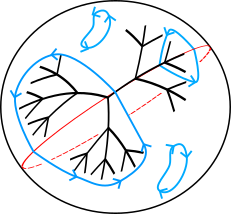
For any , Liokumovich constructed a Riemannian 2-sphere of diameter at most 1 for which [34, pg. 2]. is roughly constructed as follows. Take a unit disk in a hyperbolic plane, and embed a regular ternary tree with unit edge length and height in . Glue to a small tubular neighbourhood of the tree in by identifying their boundaries. (The curvature of must be chosen such that the boundaries have the same length.) The result is (see fig. 1(a)).
The metric of has the symmetries of an equilateral triangle, generated by reflections and rotations. A plane of reflection cuts into two isometric Riemannian disks, one of which we denote by (see fig. 1(b)). It can be verified that .
| (a) | (b) |
 |
 |
| (c) | (d) |
 |
 |
The key property of is that it has a small diameter but large width:
Lemma 2.1.
For any , there exists some such that .
Proof.
Consider a sweepout by relative 1-cycles ; unpacking the definition, this implies that for some loop , the gluing homomorphism sends to times of the fundamental class of , for some . Consider the map where the 1-cycle (see fig. 1(c)) is the double of the relative 1-cycle (see fig. 1(d)), which is obtained by subtracting a reflected copy of from . (The subtraction ensures that the orientations match up where the two copies of meet.) Then it can be verified that the gluing homomorphism sends to times of the fundamental class of . The lemma then follows from the fact that can have arbitrarily large . ∎
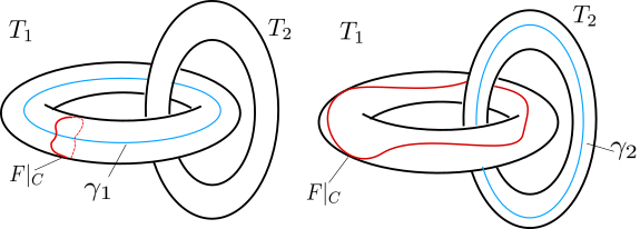
For , define to be solid tori, and let be the product metric of with a sufficiently short metric on . Embed the disjoint union into in the manner of a Hopf link (see fig. 2), and denote their union by . Cover by two open sets and so that , and let be a partition of unity subordinate to this cover. Extend over via a smooth bump function. Our Riemannian -sphere is then , where and is the metric of a round sphere of sufficiently small radius. It can be verified that .
3 Plan of the Proof of Theorem 1.1
In order to discuss the plan, we first make some notation clear. Let be a projection onto the first factor. Recall the definition of from the beginning of the Introduction. Define .
Consider a map of nonzero degree. After perturbing , each will be a smooth manifold containing a family of 1-cycles . Their images will form a sweepout of . An analysis of and the following lemma of algebraic topology guarantees the existence of a circle in some that maps to a non-contractible loop on :
Lemma 3.1.
Let be a closed, orientable, and connected surface of genus at least 1 and consider a degree nonzero map . Then for any Morse function , there exists some and a circle embedded in such that is not nullhomotopic.
This result follows from [21, Lemma 2.2]. Nevertheless, at the end of this section we will sketch a proof for the case where is a diffeomorphism, in order to articulate the fundamental reason why it is true.
As shown in fig. 2, we find that has a nonzero linking number with the core curve of either or . As a consequence of Lemma 4.3, there will exist a surface such that is contained within some . In addition, will be partitioned into the curves , and the projections of the curves onto via will give a sweepout of by relative 1-cycles. fig. 4 illustrates and , where corresponds to in the figure.
One of the curves in this sweepout by relative 1-cycles must be long, by Lemma 2.1. As these relative 1-cycles are orthogonal projections of the curves , it must be the case that some is long as well.
Proof sketch of Lemma 3.1 when is a diffeomorphism.
Since is a diffeomorphism, let us identify with . Let the critical values of be . For each , is a disjoint union of wedge sums of circles. Denote those circle wedge summands by (see fig. 3(a)). Let us assume that each circle is contractible in and derive a contradiction. In other words, we assume that each is the boundary of some 2-chain in that is the continuous image of a 2-disk (see fig. 3(c)).
We can decompose the fundamental cycle of into the sum of 2-chains for (see fig. 3(b)). Each is composed of circles (for ), and for each of these circles we can glue in . After “capping off” each circle in , becomes a 2-cycle that is the union of images of 2-spheres. To illustrate, in fig. 3(b), we can see that and have been capped off into spheres, while has been capped off into the union of two spheres.


However, as , all of these images of 2-spheres are null-homologous. If we add up all of these images of spheres, then the caps cancel each other out and the result is the fundamental cycle of . Thus we have expressed the fundamental cycle as a sum of null-homologous 2-cycles, which gives a contradiction. ∎
4 Main Result
We begin by proving that continuous maps of nonzero degree can be perturbed to “geometrically nice” maps.
Lemma 4.1.
Consider any map of nonzero degree such that every curve is shorter than for some . Then for any and any closed submanifold , is homotopic to a smooth map transverse to such that:
-
1.
For any and , the lengths of and differ by at most .
-
2.
The sets are the level sets of some Morse function on .
Proof.
We can approximate by a sequence of smooth maps for that are transverse to , so that each is a smooth manifold. It can be verified from the standard arguments for such approximations (e.g. in [30]), together with the fact that every is shorter than , that each can be chosen to satisfy (1). Thinking of as a submanifold of , the function defined by is Morse for generic [41, p. 36]. Let us pick ; then the rotational symmetry of implies that the level sets of are the intersections of with hyperplanes orthogonal to . Therefore we may modify and by precomposing them with an isometry that is close to the identity, until those level sets become . Finally, we may choose to be for sufficiently large . ∎
Thus we may replace by its perturbation . Henceforth we will assume that satisfies the properties in Lemma 4.1. Let . Then like any level set of a Morse function on a surface, each is a disjoint union of circles and at most one figure eight (a wedge sum of two circles).
The proofs of the following two lemmas were inspired by the proof of [21, Lemma 2.3]. However, that proof contained an inaccuracy, so we give our own proofs.
Lemma 4.2.
Suppose that one of the circles embedded in is such that has nonzero linking number with the core curve of for some . Then contains a surface such that is a nonzero map.
Proof.
Without loss of generality, assume has linking number with the core curve of . then bounds a disk in such that has intersection number with the core curve of .777With reference to Remark 1.2 about generalizations of Theorem 1.1, this is the part of our proof of Theorem 1.1 that requires the Jordan curve theorem. is a union of disjoint surfaces , each corresponding to an intersection number between and the core curve of . This is reflected in fig. 4. Then for some . Thus is the desired surface. ∎

We then use Lemma 4.2 to prove the following statement:
Lemma 4.3.
For some and for some , contains a surface such that is a nonzero map.
Proof.
Let . By Lemma 4.1 we can assume that for some Morse function . After choosing an orientation on and equipping with the preimage orientation, it can be verified that the map has degree equal to . (To see this, note that the preimages of a regular value of have neighbourhoods that are foliated by the ’s.) Consequently, for some connected component of , . Since , the genus of must be at least 1. Thus Lemma 3.1 gives some and a circle embedded in such that is not contractible in .
In other words, is a nonzero map with , where the first factor is a multiple of the generator homotopic to and the second factor is a multiple of the generator homotopic through to its core curve.
Then if , we have that has nonzero linking number with the core curve of , and so we may apply Lemma 4.2 to obtain as needed.
If , then where has a nonzero linking number with the core curve of , and so we again apply Lemma 4.2 to obtain . ∎
We have now proven the existence of a surface on that maps into one of the tori in a “nice” way. We use this property to define a continuous family of 1-cycles on and show that one of those 1-cycles must be long. This will eventually imply that one of the ’s must also be long, leading to a proof of Theorem 1.1.
Proof of Theorem 1.1.
Consider any . Consider the Riemannian 3-sphere that was constructed in Section 2, with chosen such that , as in Lemma 2.1. Suppose for the sake of contradiction that for some continuous map , every curve is shorter than . Recall that by applying a perturbation, we may assume that satisfies the properties of Lemma 4.1, for some . We will arrive at a contradiction by proving that some (for the perturbed ) is longer than .
Applying Lemma 4.3, we obtain a surface in for some such that for some , and is a nonzero map. With this, we may define a continuous family of relative 1-cycles by . Since , we can think of as a map .
We will show that gives a sweepout of by relative 1-cycles by appealing to the Almgren isomorphism theorem, which implies that there is a natural ismorphism [1].888A modern proof of the Almgren isomorphism theorem is available in [26]. is induced by “gluing” a family of relative 1-cycles in into a relative 2-cycle in (see fig. 5). Gluing together the relative 1-cycles gives , which represents a nontrivial class in because is a nonzero map. By the Almgren isomorphism theorem, represents a nonzero element of , and thus is also a nonzero map. By definition, gives a sweepout of by relative 1-cycles.


By Lemma 2.1, some must be longer than . As is an orthogonal projection of part of onto , we obtain that must be longer than as well. This gives a contradiction. ∎
5 Orthogonal Geodesic Chords
To prove Theorem 1.3, we will construct a sequence of Riemannian 3-spheres with small diameter and volume, so that and are large for some embedded 2-sphere and embedded circle . Consider three solid tori , , and embedded in and linked as shown in fig. 6. The embedded 2-sphere is chosen so that it intersects in two 2-disks. also separates into two closed 2-balls, and , so that contains in its interior. is chosen so that it links with as shown in the figure.
Similarly to our previous construction of the metric from Section 2, give each solid torus the product metric on , where the length of the is sufficiently small so that the volume of the product metric is at most . Extend this metric on to the entire as in Section 2, so that it is sufficiently small away from some open neighbourhood of . This defines a metric on with diameter and volume at most 1. As a Riemannian submanifold, has diameter at most 1 due to our choice of metric on .

Recall from the Introduction that denotes the space of piecewise smooth paths in whose endpoints lie on . One can prove that
| (5.1) |
by generalizing the proof that . Thus we have but .
Consider some continuous map that represents a nonzero class in . Similar to the discussion in the Plan of the Proof, induces a map , where for all . The quotient map can be chosen so that it sends to , where is regarded as the unit 3-disk in . Define and .
Suppose that every is shorter than for some . By taking the double of to get a map , we may apply Lemma 4.1 to conclude that for any we can approximate by a smooth map that is transverse to so that:
-
I.
For each and , the curves and differ in length by less than .
-
II.
Each set is a level set of a Morse function on .
In particular, each is a closed submanifold of , which we endow with the preimage orientation. Henceforth we will write to mean .
Lemma 5.1.
For some , the map has nonzero degree.
Proof.
The isomorphism from eq. 5.1 sends to . The Hurewicz homomorphism sends to a class . Statement (II) above implies that , where . (To see this, note that the preimages of a regular value of have neighbourhoods that are foliated by the ’s.) Therefore it suffices to prove that is an isomorphism. Consider the following commutative diagram whose rows are long exact sequences and whose columns are Hurewicz maps:
| (5.2) |
and are isomorphisms by the Hurewicz theorem. The Five Lemma implies that is also an isomorphism. (We use a stronger version of the Five Lemma [28, p. 129], in which the leftmost column is only required to be surjective and the rightmost column is only required to be injective.) ∎
Proof of Theorem 1.3.
Consider any . The Hölder inequality implies that for piecewise smooth curves parametrized over . Lemma 2.1 allows us to choose some such that . Consider the Riemannian 3-sphere defined at the beginning of this section.
Let us first prove that . Suppose for the sake of contradiction that . Then some nonzero class in is represented by a map such that each is shorter than . As explained previously, Lemma 4.1 implies that corresponds to a map satisfying statements (I) and (II), and so that every curve is shorter than .
Without loss of generality, Lemma 5.1 implies that has nonzero degree. An argument adapted from the proof of Lemma 4.3 implies that for some , contains some embedded circle such that is not nullhomotopic. Thus winds around the core curve of a nonzero number of times, where or 3. (Here we used the fact that and are linked.) Let denote the canonical projection. The proof of Lemma 4.2 works nearly verbatim to prove that contains a surface such that is a nonzero map. (The crucial fact is that bounds a disk in .)
As in the proof of Theorem 1.1, is swept out by a family of relative 1-cycles so as a consequence of Lemma 2.1, one of the curves must be longer than , giving a contradiction.
Next we prove that . Note that , so we consider a map of pairs that represents a nonzero class in . Suppose for the sake of contradiction that every curve has length at most . Similar to previous arguments, induces a map , where for all . The quotient map can be chosen to send to . represents a nonzero class in , and each has length at most .
The long exact sequence of homotopy groups of the pair reveals that the boundary map is an isomorphism, so winds around a nonzero number of times. Since is linked with the core curve of , the surface has a nonzero intersection number with that core curve. Similarly to the previous arguments, can be perturbed to a homotopic map that is transverse to while changing the lengths of the curves only slightly. The argument used to prove Lemma 4.2 implies the existence of some surface such that is a nonzero map. As before, is now swept out by relative 1-cycles , and similar arguments as before show that one of the curves must be longer than , giving a contradiction. ∎
Acknowledgements
The authors would like to thank Regina Rotman for suggesting the problem to us, and for helpful conversations. The first author was supported by the University of Toronto Excellence Award. The second author was supported by the Vanier Canada Graduate Scholarship.
References
- [1] F. J. Almgren, Jr. The homotopy groups of the integral cycle groups. Topology, 1:257–299, 1962.
- [2] F. Balacheff and S. Sabourau. Diastolic and isoperimetric inequalities on surfaces. Ann. Sci. Éc. Norm. Supér. (4), 43(4):579–605, 2010.
- [3] W. Ballmann, G. Thorbergsson, and W. Ziller. Existence of closed geodesics on positively curved manifolds. J. Differential Geometry, 18(2):221–252, 1983.
- [4] I. Beach. Short simple geodesic loops on a 2-sphere, 2024. Preprint.
- [5] I. Beach. Short simple orthogonal geodesic chords on a 2-disk with convex boundary, 2024.
- [6] I. Beach, H. C. Peruyero, E. Griffin, M. Kerr, R. Rotman, and C. Searle. Lengths of the orthogonal geodesic chords on riemannian manifolds, 2024.
- [7] W. Bos. Kritische Sehnen auf Riemannschen Elementarraumstücken. Math. Ann., 151:431–451, 1963.
- [8] R. Bott. Lectures on Morse theory, old and new. In Proceedings of the 1980 Beijing Symposium on Differential Geometry and Differential Equations, Vol. 1, 2, 3 (Beijing, 1980), pages 169–218. Science Press, Beijing, 1982.
- [9] D. Burago and S. Ivanov. On asymptotic isoperimetric constant of tori. Geom. Funct. Anal., 8(5):783–787, 1998.
- [10] H. Y. Cheng. Curvature-free linear length bounds on geodesics in closed Riemannian surfaces. Trans. Amer. Math. Soc., 375(7):5217–5237, 2022.
- [11] O. Chodosh and C. Mantoulidis. The -widths of a surface. Publ. Math. Inst. Hautes Études Sci., 137:245–342, 2023.
- [12] F. Codá Marques. Minimal surfaces: variational theory and applications. In Proceedings of the International Congress of Mathematicians—Seoul 2014. Vol. 1, pages 283–310. Kyung Moon Sa, Seoul, 2014.
- [13] F. Codá Marques and A. Neves. Existence of infinitely many minimal hypersurfaces in positive Ricci curvature. Invent. Math., 209(2):577–616, 2017.
- [14] C. B. Croke. Area and the length of the shortest closed geodesic. J. Differential Geom., 27(1):1–21, 1988.
- [15] C. B. Croke and M. Katz. Universal volume bounds in Riemannian manifolds. In Surveys in differential geometry, Vol. VIII (Boston, MA, 2002), volume 8 of Surv. Differ. Geom., pages 109–137. Int. Press, Somerville, MA, 2003.
- [16] H. Federer and W. H. Fleming. Normal and integral currents. Ann. of Math. (2), 72:458–520, 1960.
- [17] W. H. Fleming. Flat chains over a finite coefficient group. Trans. Amer. Math. Soc., 121:160–186, 1966.
- [18] S. Frankel and M. Katz. The morse landscape of a riemannian disk. In Annales de l’institut Fourier, volume 43, pages 503–507, 1993.
- [19] R. Giambò, F. Giannoni, and P. Piccione. Orthogonal geodesic chords, brake orbits and homoclinic orbits in Riemannian manifolds. Adv. Differential Equations, 10(8):931–960, 2005.
- [20] P. Glynn-Adey and Y. Liokumovich. Width, Ricci curvature, and minimal hypersurfaces. J. Differential Geom., 105(1):33–54, 2017.
- [21] P. Glynn-Adey and Z. Zhu. Subdividing three-dimensional Riemannian disks. J. Topol. Anal., 9(3):533–550, 2017.
- [22] M. Gromov. Filling Riemannian manifolds. J. Differential Geom., 18(1):1–147, 1983.
- [23] M. Gromov. Asymptotic invariants of infinite groups. Technical report, P00001028, 1992.
- [24] L. Guth. The width-volume inequality. Geom. Funct. Anal., 17(4):1139–1179, 2007.
- [25] L. Guth. Metaphors in systolic geometry. Preprint, 2010. https://arxiv.org/abs/1003.4247.
- [26] L. Guth and Y. Liokumovich. Parametric inequalities and weyl law for the volume spectrum. Geometry & Topology. To appear.
- [27] J. Hass and P. Scott. Shortening curves on surfaces. Topology, 33(1):25–43, 1994.
- [28] A. Hatcher. Algebraic topology. Cambridge University Press, Cambridge, 2002.
- [29] D. Ko. Existence and morse index of two free boundary embedded geodesics on riemannian 2-disks with convex boundary, 2023. Preprint.
- [30] J. M. Lee. Introduction to smooth manifolds, volume 218 of Graduate Texts in Mathematics. Springer, New York, second edition, 2013.
- [31] M. M.-C. Li. Free boundary minimal surfaces in the unit ball: recent advances and open questions. In Proceedings of the International Consortium of Chinese Mathematicians 2017, pages 401–435. Int. Press, Boston, MA, [2020] ©2020.
- [32] Y. Liokumovich. Spheres of small diameter with long sweep-outs. Proceedings of the American Mathematical Society, 141(1):309–312, 2013.
- [33] Y. Liokumovich. Slicing a 2-sphere. J. Topol. Anal., 6(4):573–590, 2014.
- [34] Y. Liokumovich. Surfaces of small diameter with large width. Journal of Topology and Analysis, 6(03):383–396, 2014.
- [35] Y. Liokumovich. Families of short cycles on Riemannian surfaces. Duke Math. J., 165(7):1363–1379, 2016.
- [36] Y. Liokumovich and D. Maximo. Waist inequality for 3-manifolds with positive scalar curvature. In Perspectives in scalar curvature. Vol. 2, pages 799–831. World Sci. Publ., Hackensack, NJ, [2023] ©2023.
- [37] Y. Liokumovich, A. Nabutovsky, and R. Rotman. Contracting the boundary of a riemannian 2-disc. Geometric and Functional Analysis, 25:1543–1574, 2015.
- [38] Y. Liokumovich and X. Zhou. Sweeping out 3-manifold of positive Ricci curvature by short 1-cycles via estimates of min-max surfaces. Int. Math. Res. Not. IMRN, (4):1129–1152, 2018.
- [39] L. Lyusternik and L. Schnirelmann. Topological methods in variational problems and their application to the differential geometry of surfaces. Uspehi Matem. Nauk (N.S.), 2(1(17)):166–217, 1947.
- [40] L. A. Lyusternik and A. I. Fet. Variational problems on closed manifolds. Doklady Akad. Nauk SSSR (N.S.), 81:17–18, 1951.
- [41] J. Milnor. Morse theory, volume No. 51 of Annals of Mathematics Studies. Princeton University Press, Princeton, NJ, 1963. Based on lecture notes by M. Spivak and R. Wells.
- [42] A. Nabutovsky. Linear bounds for constants in Gromov’s systolic inequality and related results. Geom. Topol., 26(7):3123–3142, 2022.
- [43] A. Nabutovsky and R. Rotman. The length of the shortest closed geodesic on a 2-dimensional sphere. Int. Math. Res. Not., (23):1211–1222, 2002.
- [44] A. Nabutovsky and R. Rotman. Upper bounds on the length of a shortest closed geodesic and quantitative Hurewicz theorem. J. Eur. Math. Soc. (JEMS), 5(3):203–244, 2003.
- [45] A. Nabutovsky and R. Rotman. Linear bounds for lengths of geodesic loops on Riemannian 2-spheres. J. Differential Geom., 89(2):217–232, 2011.
- [46] A. Nabutovsky and R. Rotman. Length of geodesics and quantitative Morse theory on loop spaces. Geom. Funct. Anal., 23(1):367–414, 2013.
- [47] A. Nabutovsky, R. Rotman, and S. Sabourau. Sweepouts of closed Riemannian manifolds. Geom. Funct. Anal., 31(3):721–766, 2021.
- [48] A. Neves. New applications of min-max theory. In Proceedings of the International Congress of Mathematicians—Seoul 2014. Vol. II, pages 939–957. Kyung Moon Sa, Seoul, 2014.
- [49] A. Oancea. Morse theory, closed geodesics, and the homology of free loop spaces. In Free loop spaces in geometry and topology, volume 24 of IRMA Lect. Math. Theor. Phys., pages 67–109. Eur. Math. Soc., Zürich, 2015. With an appendix by Umberto Hryniewicz.
- [50] P. Papasoglu. Contracting thin disks. J. Topol. Anal., 11(4):965–970, 2019.
- [51] P. Papasoglu and E. Swenson. A surface with discontinuous isoperimetric profile and expander manifolds. Geom. Dedicata, 206:43–54, 2020.
- [52] H.-B. Rademacher. Upper bounds for the critical values of homology classes of loops. Manuscripta Math., 174(3-4):891–896, 2024.
- [53] R. Rotman. The length of a shortest closed geodesic and the area of a 2-dimensional sphere. Proc. Amer. Math. Soc., 134(10):3041–3047, 2006.
- [54] R. Rotman. Positive Ricci curvature and the length of a shortest periodic geodesic. J. Geom. Anal., 34(6):Paper No. 167, 27, 2024.
- [55] S. Sabourau. Filling radius and short closed geodesics of the 2-sphere. Bull. Soc. Math. France, 132(1):105–136, 2004.
- [56] S. Sabourau. Volume of minimal hypersurfaces in manifolds with nonnegative Ricci curvature. J. Reine Angew. Math., 731:1–19, 2017.
- [57] J.-P. Serre. Homologie singulière des espaces fibrés. Applications. Ann. of Math. (2), 54:425–505, 1951.
- [58] A. Treibergs. Estimates of volume by the length of shortest closed geodesics on a convex hypersurface. Invent. Math., 80(3):481–488, 1985.
- [59] A. S. Švarc. Geodesic arcs on Riemann manifolds. Uspehi Mat. Nauk, 13(6(84)):181–184, 1958.
- [60] N. Wu and Z. Zhu. Length of a shortest closed geodesic in manifolds of dimension four. J. Differential Geom., 122(3):519–564, 2022.
- [61] X. Zhou. On the free boundary min-max geodesics. Int. Math. Res. Not. IMRN, (5):1447–1466, 2016.