Revival of oscillation and symmetry breaking in coupled quantum oscillators

Biswabibek Bandyopadhyay Chaos and Complex Systems Research Laboratory, Department of Physics, University of Burdwan, Burdwan 713 104, West Bengal, India Tanmoy Banerjee [email protected] Chaos and Complex Systems Research Laboratory, Department of Physics, University of Burdwan, Burdwan 713 104, West Bengal, India

Abstract

Restoration of oscillation from an oscillation suppressed state in coupled oscillators is an important topic of research and has been studied widely in recent years. However, the same in the quantum regime has not been explored yet. Recent works established that under certain coupling conditions coupled quantum oscillators are susceptible to suppression of oscillations, such as amplitude death and oscillation death. In this paper, for the first time we demonstrate that quantum oscillation suppression states can be revoked and rhythmogenesis can be established in coupled quantum oscillators by controlling a feedback parameter in the coupling path. However, in sharp contrast to the classical system, we show that in the deep quantum regime the feedback parameter fails to revive oscillation, rather results in a transition from quantum amplitude death state to the recently discovered quantum oscillation death state. We use the formalism of open quantum system and phase space representation of quantum mechanics to establish our results. Therefore, our study establishes that revival scheme proposed for classical systems does not always result in restoration of oscillation in quantum systems but in the deep quantum regime it may give counterintuitive behaviors that are of pure quantum mechanical origin.

Understanding dissipative nonlinear systems in the quantum regime has recently been identified as an important topic of research. In the quantum domain the well known phenomena like synchronization and oscillation quenching show several significant results that have no counterpart in the classical domain. In this context, the restoration of oscillation from an oscillation suppressed state in coupled oscillators has not been explored yet in the quantum regime. In this paper, for the first time we study the phenomenon of revoking quantum oscillation suppression states. We demonstrate that in the weak quantum regime the revival mechanism works properly. However, in sharp contrast to the classical system, we show that in the deep quantum regime, the process of rhythmogenesis fails, and results in a transition from quantum amplitude death state to quantum oscillation death state. We use the formalisms used in open quantum systems and noisy classical systems to establish our results.

I Introduction

Exploring nonlinear dynamics in the open quantum systems has gained much attention in recent years Lee and Sadeghpour (2013); Walter, Nunnenkamp, and Bruder (2014); Laskar et al. (2020); Koppenhöfer, Bruder, and Roulet (2020). The well known concepts of nonlinear dynamics such as oscillation of a single unit, and emergent behaviors of coupled oscillatory units, such as synchronization Pikovsky, Rosenblum, and Kurths (2003) have recently been explored in the quantum regime Lee and Sadeghpour (2013); Walter, Nunnenkamp, and Bruder (2014). The extension of the techniques used in the so called classical nonlinear dynamics to the quantum regime is not always straightforward. Understanding of nonlinear behavior in the quantum domain is based on the formalism of open quantum system that requires the solution of quantum master equations Carmichael (1999). Also, phase space representation of quantum system which involves quasi probability function (e.g. Wigner function Weinbub and Ferry (2018)) plays a crucial role in this endeavor.

Nonlinear dynamics in the quantum regime is worth studying as the well known classical results deviate in the quantum regime and manifest several counterintuitive results that are not possible in the classical system. The notion of synchronization in the quantum regime is explored in detail both theoretically Lee and Sadeghpour (2013); Walter, Nunnenkamp, and Bruder (2014) and experimentally Laskar et al. (2020); Koppenhöfer, Bruder, and Roulet (2020). Refs. Lee and Sadeghpour, 2013 and Walter, Nunnenkamp, and Bruder, 2014 explored the role of the inherent quantum noise to defy synchronization in the quantum regime: Later on, several aspects of quantum synchronization Lee, Chan, and Wang (2014); Walter, Nunnenkamp, and Bruder (2015); Lörch et al. (2017); Morgan and Hinrichsen (2015) and to improve the quality of synchronization Sonar et al. (2018); Mok, Kwek, and Heimonen (2020) have been reported. The manifestation of partial synchronization or chimera state Zakharova (2020); Banerjee et al. (2018a); Poel, Zakharova, and Schöll (2015) differs in the quantum regimeBastidas et al. (2015). In the context of control, the well known Pyragas control scheme Pyragas (1992) has been tested in the quantum regime Droenner et al. (2019). The phenomenon of coherence resonance has been found to deviate in the quantum regime and shows improvement of regular behavior in the presence of inherent quantum noise Kato and Nakao (2021) Subsequently, quantum manifestation of another widely studied emergent dynamics, namely oscillation quenching has also been studied recently. Ishibashi et. al. Ishibashi and Kanamoto (2017) demonstrated that, similar to classical system, in quantum oscillators also parameter mismatch in diffusive coupling leads to amplitude death (AD) where all the oscillators arrive at the common steady state. However, unlike classical system, complete suppression of oscillation is restricted by the inherent quantum noise present in the quantum oscillators. Nevertheless, a pronounced decrease in the mean boson number is found to be indicative of quantum AD. Later, Amitai et. al. Amitai et al. (2018) showed that the Kerr-type anharmonicity is conducive to quantum AD. Apart from AD there exists a symmetry-breaking version of oscillation suppression called oscillation death (OD) in which coupling dependent nontrivial steady states are created Koseska, Volkov, and Kurths (2013a, b); recently Bandyopadhyay et al. (2020) discovered the quantum analogue of the OD state.

In this context an important emergent dynamics, namely the revival of oscillation from the oscillation suppressed state has yet not been explored in the quantum regime. Revival of oscillation is important in several physical and biological systems as maintaining rhythmicity is often desirable in those systems. Examples include power grid, El nino, sinuartial rhythm where cessation of oscillations may cause serious consequences. Several techniques of revival of oscillations have been proposed in the literature all of which are based on either controlling the delay or the dissipation rate of the coupling function. The most general technique of revival of oscillation has been reported by Zou et. al. Zou et al. (2015) that is based on the introduction of a feedback parameter in the coupling path. This technique modifies the dissipation rate in the coupling path and works successfully over a broad range of coupling functions and oscillators Ghosh, Banerjee, and Kurths (2015). However, all these revival schemes are studied in the classical regime.

In this paper, for the first time, we study the revival of oscillations in the hitherto unexplored quantum regime. Our main aim in this paper is to test the applicability and efficacy of the “dissipation-modified” revival scheme of Ref. Zou et al., 2015; Ghosh, Banerjee, and Kurths, 2015. For our study we consider the paradigmatic quantum van der Pol oscillators with a coupling scheme, which is known to induce “death”, namely the mean-field diffusive coupling Banerjee (2015); Banerjee, Dutta, and Gupta (2015). We show that revival of oscillation from quantum amplitude death state is indeed possible in the weak quantum regime. The revival of oscillation is manifested by the pronounced increase in the mean phonon number. However, in sharp contrast to the classical and weak quantum case, in the deep quantum regime the technique does not result in revival of oscillation, rather the system is trapped in either homogeneious or inhomogeneous quantum steady states; the variation of the feedback parameter results in a transition from quantum AD state to the quantum OD state that has no counterpart in the semiclassical regime. The present study asserts that the revival of oscillations manifests results that are exclusive to quantum domain only.

The rest of the paper is organized as follows: the next section provides the mathematical model and manifestation of oscillation of a single quantum van der Pol oscillator. Section III presents the classical revival scheme in coupled oscillators under mean-field diffusive coupling. Section IV describes the revival and symmetry breaking phenomena in coupled quantum oscillators; it formulates the quantum master equation and the results of weak and deep quantum quantum regime. In the weak quantum regime a semiclassical treatment with noisy classical model is also presented in this section. Finally, we summarize the results in Sec. V.

Refer to caption — Figure 1: Limit cycle from quantum van der Pol oscillator (Eq. 3). (a) Weak quantum regime: $k_{1}=1$ and $k_{2}=0.2$ . (b) Deep quantum regime: $k_{1}=1$ , and $k_{2}=3$ . ( $\omega=2$ ).

II Quantum van der Pol oscillator

Let us at first describe a single van der Pol oscillator in the classical and quantum domain. A classical van der Pol oscillator has the following mathematical form van der Pol (1922); Walter, Nunnenkamp, and Bruder (2014):


$\displaystyle\dot{x}$	$\displaystyle=\omega y,$	(1a)
$\displaystyle\dot{y}$	$\displaystyle=-\omega x+(k_{1}-8k_{2}{x}^{2})y,$	(1b)

where $\omega$ is the eigenfrequency of the oscillator. $k_{1}$ and $k_{2}$ control the linear gain and the nonlinear damping, respectively ( $k_{1},k_{2}>0$ ). By using harmonic approximationsBandyopadhyay et al. (2020) we derive the following amplitude equation of Eq. (1) in terms of a complex amplitude, $\alpha=x+iy$ :

\dot{\alpha}=-i\omega\alpha+(\frac{k_{1}}{2}-k_{2}|\alpha|^{2})\alpha.

(2)

The oscillator shows a limit cycle oscillation with an amplitude $\sqrt{\frac{k_{1}}{2k_{2}}}$ .

Let us write the quantum master equation corresponding to the quantum van der Pol oscillator Lee and Sadeghpour (2013); Walter, Nunnenkamp, and Bruder (2014):

\dot{\rho}=-i[\omega a^{\dagger}a,\rho]+k_{1}\mathcal{D}[a^{\dagger}](\rho)+k_{2}\mathcal{D}[a^{2}](\rho).

(3)

This equation actually represents a harmonic oscillator interacting with the environment (bath) through the Lindblad dissipator $\mathcal{D}[\hat{O}](\rho)$ : where $\mathcal{D}[\hat{O}](\rho)=\hat{O}\rho\hat{O}^{\dagger}-\frac{1}{2}\{\hat{O}^{\dagger}\hat{O},\rho\}$ (we consider $\hbar=1$ ). $a$ and $a^{\dagger}$ are the bosonic annihilation and creation operators, respectively. $k_{1}$ is the linear pumping rate that controls the creation of a single boson and $k_{2}$ represents the nonlinear loss rate governing the annihilation of two bosons. Eq. 3 has been widely studied in the context of synchronization and oscillation suppression. In the classical limit (or weak quantum limit), linear pumping ( $k_{1}$ ) dominates over the nonlinear loss (i.e., $k_{1}>k_{2}$ ) and in this higher excitation region one can consider $\langle a\rangle\equiv\alpha$ , and the master equation (3) and the classical amplitude equation (2) are equivalent through the following relation: $\dot{\braket{a}}=\mbox{Tr}(\dot{\rho}a)$ . Figure 1(a) shows the steady state Wigner function based phase space representation of the quantum limit cycle (using QuTiP Johansson, Nation, and Nori (2013)) in the weak quantum limit ( $k_{1}=1$ and $k_{2}=0.2$ ). In the limit where $k_{2}>k_{1}$ the system resides in the deep quantum regime. In this limit only a few Fock levels near the quantum mechanical ground state are populated: Fig. 1(b) shows the corresponding limit cycle for $k_{1}=1$ and $k_{2}=3$ . In the limiting case of $k_{2}\rightarrow\infty$ the steady state density matrix is Lee and Sadeghpour (2013) $\rho_{ss}=\frac{2}{3}|0\rangle\langle 0|+\frac{1}{3}|1\rangle\langle 1|$ . i.e., the oscillation still persists unlike classical vdP oscillator.

III Classical Revival of oscillation

Before proceed to the quantum case, let us demonstrate the revival scheme of two identical classical van der Pol oscillators that are coupled via weighted mean-field diffusive coupling. A mathematical model is given byBandyopadhyay et al. (2020)


$\displaystyle\dot{x}_{j}$	$\displaystyle=\omega y_{j}+\varepsilon\left(\frac{q}{2}\sum_{m=1}^{2}x_{m}-\upgamma x_{j}\right),$	(4a)
$\displaystyle\dot{y}_{j}$	$\displaystyle=-\omega x_{j}+(k_{1}-8k_{2}{x_{j}}^{2})y_{j},$	(4b)

$j\in\{1,2\}$ . $\varepsilon$ is the coupling parameter. Both the oscillators have the common eigenfrequency $\omega$ . The control parameter $q$ determines the density of the weighted mean-field, which is relevant in several processes including quantum physics Bandyopadhyay et al. (2020) and biology Ullner et al. (2007). Here the parameter $\upgamma$ controls the dissipation rate in the coupling part: it actually controls the asymmetry between the incoming and outgoing flow of the diffusion processZou et al. (2015). $\upgamma=1$ represents the normal mean-field diffusive coupling. By decreasing $\upgamma$ below unity ( $0<\upgamma<1$ ) one reduces the dissipation rate in the coupling channel which is conducive for rhythmic behavior Zou et al. (2015); Ghosh, Banerjee, and Kurths (2015). The introduction of $\upgamma$ is especially relevant in the open quantum systems as here the dynamics is essentially dissipative.

The system Eq. 4 has two types of fixed points, namely trivial fixed point $\mathcal{F}_{HSS}\equiv(0,0,0,0)$ and nontrivial fixed point $\mathcal{F}_{IHSS}=(x^{*},y^{*},-x^{*},-y^{*})$ , where $x^{*}=\frac{\omega y^{*}}{\varepsilon\upgamma}$ and $y^{*}=\pm\sqrt{\frac{1}{8k_{2}}\left(\frac{k_{1}\varepsilon^{2}\upgamma^{2}}{\omega^{2}}-\varepsilon\upgamma\right)}$ . The system shows a transition from oscillatory state to amplitude death state through an inverse Hopf bifurcation at $\varepsilon_{\mbox{HB}}=\frac{k_{1}}{(\upgamma-q)}$ Banerjee and Ghosh (2014a, b). The classical equation Eq. (4) shows a transition from AD to OD state through a pitchfork bifurcation at $\epsilon_{\mbox{PB}}=\frac{\omega^{2}}{k_{1}\upgamma}$ Banerjee and Ghosh (2014a, b). The Hopf and pitchfork bifurcation curves in the $\varepsilon/k_{1}-\upgamma$ space are shown in Fig. 2 ( $q=0.2$ ). In the classical model above the Hopf bifurcation curve (HB) amplitude death occurs. However, if one decreases the control parameter $\upgamma$ , below the HB curve the death state is revoked and oscillatory behavior is restored. Therefore, the HB curve is the oscillation revival curve. In the next section we discuss how this revival scenario holds in quantum systems.

IV Pure Quantum Model: Revival and symmetry breaking

IV.1 quantum master equation

The quantum master equation of two scalar mean-field diffusively coupled identical quantum van der Pol oscillators under revival scheme is given by,

\begin{split}\dot{\rho}&=-i\bigg{[}\omega(a_{1}^{\dagger}a_{1}+a_{2}^{\dagger}a_{2})+\frac{i\epsilon}{4}\big{(}q(a_{1}^{\dagger}a_{2}^{\dagger}-a_{1}a_{2})\\ &+(\frac{q}{2}-\upgamma)({a_{1}^{\dagger}}^{2}+{a_{2}^{\dagger}}^{2}-{a_{1}}^{2}-{a_{2}}^{2})\big{)},\rho\bigg{]}\\ &+k_{1}\sum_{j=1}^{2}\mathcal{D}[a_{j}^{\dagger}](\rho)+k_{2}\sum_{j=1}^{2}\mathcal{D}[{a_{j}}^{2}](\rho)\\ &+\frac{q\epsilon}{2}\mathcal{D}[(a_{1}+a_{2})^{\dagger}](\rho)+\epsilon\upgamma\sum_{j=1}^{2}\mathcal{D}[a_{j}](\rho).\end{split}

(5)

where $a_{j}$ ( $a_{j}^{\dagger}$ ) is the annihilation (creation) operator corresponding to the $j$ -th oscillator. In the classical limit ( $k_{1}>k_{2}$ ), using the relation $\dot{\braket{a}}=\mbox{Tr}(\dot{\rho}a)$ , the master equation (5) is equivalent to the classical amplitude equation of Eq. (4), which reads

\begin{split}\dot{\alpha_{j}}&=-i\omega\alpha_{j}+(\frac{k_{1}}{2}-k_{2}|\alpha_{j}|^{2})\alpha_{j}+\frac{\varepsilon}{2}\left(\frac{q}{2}\sum_{m=1}^{2}\alpha_{m}-\upgamma\alpha_{j}\right)\\ &+\frac{\varepsilon}{2}\left(\frac{q}{2}\sum_{m=1}^{2}\alpha^{*}_{m}-\upgamma\alpha^{*}_{j}\right).\end{split}

(6)

IV.2 Weak quantum regime: revival of oscillations

IV.2.1 Quantum results

At first, we consider the weak quantum regime where excitations are moderate or large. We ensure this region by taking the pumping rate ( $k_{1}$ ) higher than the damping rate ( $k_{2}$ ). We solve the master equation (5) numerically using QuTiP Johansson, Nation, and Nori (2013) for the following parameters: $k_{1}=1$ and $k_{2}=0.2$ . Fig. 2 (a) shows the color map of the mean phonon number of the first oscillator ( $\braket{a_{1}^{\dagger}a_{1}}$ ) in the $\varepsilon/k_{1}-\upgamma$ space at $q=0.2$ . It can be seen from the figure that for $\upgamma=1$ quantum amplitude death (QAD) occurs for $\varepsilon/k_{1}>\varepsilon_{\mbox{HB}}/k_{1}$ . This is manifested by the pronounced decrease of mean phonon number ( $\braket{a_{1}^{\dagger}a_{1}}$ ) with increasing $\varepsilon/k_{1}$ (see the inset of Fig. 2 (a)). The corresponding Wigner function is shown in Fig. 2 (b) that depicts a squeezed quantum AD state for $\upgamma=1$ and $\varepsilon/k_{1}=3.5$ . Compare it with the limit cycle of Fig. 1(a) (for $\upgamma=1$ and $\varepsilon/k_{1}=0$ ) where the Wigner function shows maximum distribution at values far from the origin, however, in the quantum AD state the Wigner function shows maximum probability around the origin indicating sharp decrease in amplitude. However, the inherent quantum noise resists the complete cessation of amplitude.

This quantum AD state can be revoked by decreasing the dissipation parameter $\upgamma$ . We find that by decreasing $\upgamma$ value from a point above the HB curve (i.e., quantum AD state) we can enter into the quantum oscillatory region (below the HB curve) at a particular value of $\varepsilon/k_{1}$ . From Fig. 2 (a) it can be seen that decrease in $\upgamma$ below the HB curve results in the pronounced increase in the mean phonon number. This is demonstrated for an exemplary value of $\upgamma=0.2$ and $\varepsilon/k_{1}=3.5$ in Fig. 2 (c). In contrast to Fig. 2 (b) ( $\upgamma=1$ ), Fig. 2 (c) shows a Wigner distribution that resides around the non-zero values indicating the occurrence of quantum limit cycle. Therefore, $\upgamma$ acts as a control parameter and responsible for the occurrence of revival of quantum oscillation. However, in agreement with Ref. Bandyopadhyay et al., 2020 we do not get any quantum OD state in the weak quantum regime even in the presence of the dissipation parameter $\upgamma$ . Therefore, the classical PB curve does not play any role in the weak quantum region.

IV.2.2 Noisy classical results

For better understanding of the revival phenomenon we study the noisy classical model and compare the results with that of quantum systems. In both the cases equal noise intensity has to be considered. For this, the quantum master equation (5) is represented in phase space using partial differential equation of Wigner distribution function Carmichael (1999).

\begin{split}\dot{W}&=\sum_{j=1}^{2}\left[-\left(\frac{\partial}{\partial\alpha_{j}}\mu_{\alpha_{j}}+c.c.\right)\right.\\ &+\left.\frac{1}{2}\left(\frac{\partial^{2}}{\partial\alpha_{j}\partial{\alpha_{j}}^{*}}D_{\alpha_{j}{\alpha_{j}}^{*}}+\frac{\partial^{2}}{\partial\alpha_{j}\partial{\alpha_{j^{\prime}}}^{*}}D_{\alpha_{j}{\alpha_{j^{\prime}}}^{*}}\right)\right.\\ &+\left.\frac{k_{2}}{4}\left(\frac{\partial^{3}}{\partial{\alpha_{j}}^{*}\partial{\alpha_{j}}^{2}}\alpha_{j}+c.c\right)\right]W,\end{split}

(7)

where $\mu$ and $D$ are respectively the elements of drift vector and diffusion matrix. Here, $\mu_{\alpha_{j}}=\left[-i\omega+\frac{k_{1}}{2}-k_{2}(|\alpha_{j}|^{2}-1)\right]\alpha_{j}-\left(\frac{\varepsilon\upgamma}{2}-\frac{\varepsilon q}{4}\right)(\alpha_{j}+{\alpha_{j}}^{*})+\frac{\varepsilon q}{4}(\alpha_{j^{\prime}}+{\alpha_{j^{\prime}}}^{*})$ , $D_{\alpha_{j}{\alpha_{j}}^{*}}=k_{1}+2k_{2}(2|\alpha_{j}|^{2}-1)+\frac{\varepsilon q}{2}+\varepsilon\upgamma$ and $D_{\alpha_{j}{\alpha_{j^{\prime}}}^{*}}=\frac{\varepsilon q}{2}$ with $j=1,2$ , $j^{\prime}=1,2$ and $j\neq j^{\prime}$ . In weak nonlinear regime ( $k_{2}<k_{1}$ ), the third-order terms can be ignored and this differential equation is reduced to the Fokker-Planck equation, which is given below for our system:

\begin{split}\dot{W}(\textbf{X})&=\sum_{j=1}^{2}\left[-\left(\frac{\partial}{\partial x_{j}}\mu_{x_{j}}+\frac{\partial}{\partial y_{j}}\mu_{y_{j}}\right)\right.\\ &+\left.\frac{1}{2}\left(\frac{\partial^{2}}{\partial x_{j}\partial x_{j}}D_{x_{j}x_{j}}+\frac{\partial^{2}}{\partial y_{j}\partial y_{j}}D_{y_{j}y_{j}}\right.\right.\\ &+\left.\left.\frac{\partial^{2}}{\partial x_{j}\partial x_{j^{\prime}}}D_{x_{j}x_{j^{\prime}}}+\frac{\partial^{2}}{\partial y_{j}\partial y_{j^{\prime}}}D_{y_{j}y_{j^{\prime}}}\right)\right]W(\textbf{X}),\end{split}

(8)

where $\textbf{X}=(x_{1},y_{1},x_{2},y_{2})$ . The elements of drift vector are,


	$\displaystyle\begin{split}\mu_{x_{j}}&=\omega y_{j}+\left[\frac{k_{1}}{2}-k_{2}({x_{j}}^{2}+{y_{j}}^{2}-1)\right.\\ &-\left.\left(\varepsilon\upgamma-\frac{\varepsilon q}{2}\right)\right]x_{j}+\frac{\varepsilon q}{2}x_{j^{\prime}},\end{split}$			(9a)
	$\displaystyle\begin{split}\mu_{y_{j}}&=-\omega x_{j}+\left[\frac{k_{1}}{2}-k_{2}({x_{j}}^{2}+{y_{j}}^{2}-1)\right]y_{j}.\end{split}$			(9b)

The diffusion matrix has the following form,

	D	$\displaystyle=\left(\begin{array}[]{cccc}D_{x_{1}x_{1}}&0&D_{x_{1}x_{2}}&0\\ 0&D_{y_{1}y_{1}}&0&D_{y_{1}y_{2}}\\ D_{x_{2}x_{1}}&0&D_{x_{2}x_{2}}&0\\ 0&D_{y_{2}y_{1}}&0&D_{y_{2}y_{2}}\end{array}\right)$		(14)
		$\displaystyle=\frac{1}{2}\left(\begin{array}[]{cccc}\nu_{1}&0&\frac{\varepsilon q}{4}&0\\ 0&\nu_{1}&0&\frac{\varepsilon q}{4}\\ \frac{\varepsilon q}{4}&0&\nu_{2}&0\\ 0&\frac{\varepsilon q}{4}&0&\nu_{2}\end{array}\right),$		(19)

where $\nu_{j}=\frac{k_{1}}{2}+k_{2}[2({x_{j}}^{2}+{y_{j}}^{2})-1]+\frac{\varepsilon q}{4}+\frac{\varepsilon\upgamma}{2}$ .

From Eq.(8) the following stochastic differential equation can be derived:

d\textbf{X}=\bm{\mu}dt+\bm{\sigma}d\textbf{W}_{t},

(20)

where $\bm{\sigma}$ is the noise strength and $d\textbf{W}_{t}$ is the Wiener increment. As the diffusion matrix D (given in Eq.(14)) is symmetric, we can analytically derive $\bm{\sigma}$ from it. First, D has to be diagonalized. The diagonal form of D can be written as $\textbf{D}_{diag}=\textbf{U}^{-1}\textbf{D}\textbf{U}=diag(\lambda_{-}\lambda_{-}\lambda_{+}\lambda_{+})$ . Where $\lambda_{\pm}=\frac{1}{4}\left[\nu_{1}+\nu_{2}\pm\sqrt{(\nu_{1}-\nu_{2})^{2}+(\frac{\varepsilon q}{2})^{2}}\right]$ and U has the following form:

\displaystyle=\left(\begin{array}[]{cccc}0&u_{-}&0&u_{+}\\ u_{-}&0&u_{+}&0\\ 0&1&0&1\\ 1&0&1&0\end{array}\right),

(25)

where $u_{\pm}=\frac{2}{\varepsilon q}\left[\nu_{1}-\nu_{2}\pm\sqrt{(\nu_{1}-\nu_{2})^{2}+(\frac{\varepsilon q}{2})^{2}}\right]$ . Now, $\bm{\sigma}$ matrix can be evaluated from the equation $\bm{\sigma}=\textbf{U}\sqrt{\textbf{D}_{diag}}\textbf{U}^{-1}$ and it has the following form:

\displaystyle\bm{\sigma}

\displaystyle=\left(\begin{array}[]{cccc}\sigma_{1}&0&\sigma_{3}&0\\ 0&\sigma_{1}&0&\sigma_{3}\\ \sigma_{3}&0&\sigma_{2}&0\\ 0&\sigma_{3}&0&\sigma_{2}\end{array}\right),

(30)

where $\sigma_{1}=\frac{u_{+}\sqrt{\lambda_{+}}-u_{-}\sqrt{\lambda_{-}}}{u_{+}-u_{-}}$ , $\sigma_{2}=\frac{u_{+}\sqrt{\lambda_{-}}-u_{-}\sqrt{\lambda_{+}}}{u_{+}-u_{-}}$ and $\sigma_{3}=\frac{\sqrt{\lambda_{+}}-\sqrt{\lambda_{-}}}{u_{+}-u_{-}}$ .

By solving the stochastic differential equation (Eq. (20)) (using JiTCSDE module in Python Ansmann (2018)) we compute the ensemble average of the squared steady-state amplitude of the first oscillator ( $\overline{{|\alpha_{1}|_{nc}}^{2}}$ ), averaged over 1000 realizations, starting from random initial conditions.

Fig. 3 shows the plots of average amplitude and mean phonon number in classical, noisy classical and quantum oscillators with the variation of $\upgamma$ at $\varepsilon/k_{1}=3.5$ and $q=0.2$ (along the vertical line of Fig. 2(a)). At this value, $\upgamma=1$ gives amplitude death in all the three cases. The classical AD state shows zero amplitude, i.e, $\overline{{|\alpha_{1}|}^{2}}=0$ . However, for quantum and noisy classical cases the inherent noise resists the complete cessation of oscillation. The occupation of Fock levels at the quantum AD state is shown in the inset (right) for $\upgamma=1$ indicating the fact that the ground state is the most populated state. However, with decreasing $\upgamma$ , average amplitude and mean phonon number increase indicating revival of oscillation in classical, noisy classical and quantum systems. However, unlike the classical case no sharp transition from amplitude death state to oscillatory state is possible in quantum and noisy classical cases due to the presence of the inherent noise. The occupation of Fock levels at the revived quantum oscillatory state is shown in the inset (left) for $\upgamma=0.2$ showing that the ground state is now depleted of phonon.

IV.3 Deep quantum regime: symmetry-breaking death state

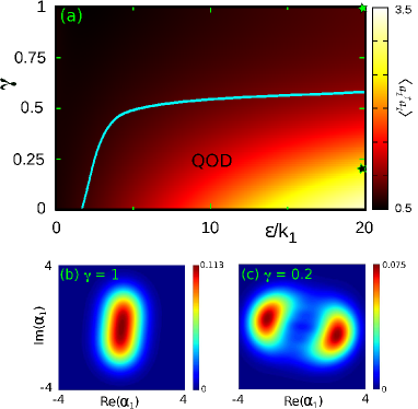
Finally, we study the effect of revival scheme in the deep quantum regime ( $k_{2}>k_{1}$ ). Surprisingly, in stark contrast to the classical case, in the deep quantum regime a decrease in the dissipation parameter $\upgamma$ does not result in the revival of oscillation, rather it leads to an interesting symmetry-breaking steady state, namely quantum oscillation death (OD) state that is manifested in the phase space through a bimodal Wigner function. This state has recently been discovered in Ref. Bandyopadhyay et al., 2020 in the deep quantum regime under mean-field diffusive coupling. In the bimodal Wigner function the two lobes are equivalent to the two branches of the pitchfork bifurcation of classical case representing inhomogeneous steady states. Figure 4(a) shows the mean phonon number ( $\braket{a_{1}^{\dagger}a_{1}}$ ) in the $\upgamma-\varepsilon/k_{1}$ space. Above the cyan curve unimodal Wigner function appears representing either quantum limit cycle or quantum AD. The quantum OD state appears below the cyan curve where the Wigner function becomes bimodal. Figure 4(b) shows the Wigner function in phase space at $\upgamma=1$ which is unimodal in nature representing quantum AD and Fig. 4(c) shows the same but for $\upgamma=0.2$ showing bimodal Wigner function representing the occurrence of quantum OD. We propose a numerical measure to mark the occurrence of quantum OD, which is based on the distance between the maximum values of the lobes of the Wigner function projected on the horizontal axis ( $\Delta X$ ) [see the inset of Fig. 5]. In the case of unimodal Wigner function $\Delta X=0$ . However, for the quantum OD, the Wigner function becomes bimodal, thus giving rise to two lobes separated by $\Delta X\neq 0$ . In Fig. 5 we plot $\Delta X$ with $\upgamma$ . It shows that in the range $\upgamma_{c}\leq\upgamma\leq 1$ the Wigner function is unimodal. However, for $\upgamma<\upgamma_{c}$ , with decreasing $\upgamma$ bimodal Wigner function appears having $\Delta X\neq 0$ mimicking symmetry-breaking classical pitchfork bifurcation and the appearance of quantum OD. However, it should be noted that in the deep quantum regime there is no one to one correspondence between the quantum and classical results.

V Conclusions

In this paper we have studied the revival of oscillation in coupled quantum oscillators by tuning a feedback parameter that controls the rate of dissipation in the coupling path. In coupled classical oscillators this was shown to be a general technique to revive oscillation from a oscillation suppressed state Zou et al. (2015); Ghosh, Banerjee, and Kurths (2015). However, we have shown that although this technique works in revival of oscillation in the weak quantum regime, in stark contrast to the classical and semiclassical results, in the deep quantum regime it fails to do so; rather in this regime it leads to a symmetry-breaking transition from homogeneous oscillation quenching state (i.e., quantum amplitude death) to inhomogeneous oscillation quenching state (i.e., quantum oscillation death state). Our results established that, unlike classical systems, controlling the dissipation rate of the coupling path is not sufficient for the revival of oscillation in the deep quantum regime.

In this paper we studied the “dissipation-modified” revival of oscillations in the quantum regime. However, we believe to get similar results in the case of other revival schemes, such as introduction of local low-pass filter Zou, Zhan, and Kurths (2017); Banerjee et al. (2018b) or time delay in the coupling path Zou et al. (2013); Biswas and Banerjee (2018), as in those cases also dissipation rate is being modified.

Apart from the academic interest, the revoking of a death state may play a crucial role in the quantum nanomechanical Bemani et al. (2017); Shim, Imboden, and Mohanty (2007) and optomechanical Jayich et al. (2008) oscillators where maintaining rhythmicity is crucial for proper functioning of the systems. Also, our study will be helpful in creating the squeezed and symmetry-breaking squeezed states that are found to be useful in several physical applications and precision measurements Lloyd and Braunstein (1999); Goda et al. (2008).

Acknowledgements.

B.B. acknowledges the financial assistance from the University Grants Commission (UGC), India. T. B. acknowledges the financial support from the Science and Engineering Research Board (SERB), Government of India, in the form of a Core Research Grant [CRG/2019/002632].

Data Availability Statement

The data that support the findings of this study are available from the corresponding author upon reasonable request.

References

Lee and Sadeghpour (2013) T. E. Lee and H. R. Sadeghpour, “Quantum synchronization of quantum van der pol oscillators with trapped ions,” Phys. Rev. Lett. 111, 234101 (2013).
Walter, Nunnenkamp, and Bruder (2014) S. Walter, A. Nunnenkamp, and C. Bruder, “Quantum synchronization of a driven self-sustained oscillator,” Phys. Rev. Lett. 112, 094102 (2014).
Laskar et al. (2020) A. W. Laskar, P. Adhikary, S. Mondal, P. Katiyar, S. Vinjanampathy, and S. Ghosh, “Observation of quantum phase synchronization in spin-1 atoms,” Phys. Rev. Lett. 125, 013601 (2020).
Koppenhöfer, Bruder, and Roulet (2020) M. Koppenhöfer, C. Bruder, and A. Roulet, “Quantum synchronization on the IBM Q system,” Phys. Rev. Research 2, 023026 (2020).
Pikovsky, Rosenblum, and Kurths (2003) A. Pikovsky, M. Rosenblum, and J. Kurths, Synchronization: A Universal Concept in Nonlinear Sciences (Cambridge University Press, England, 2003).
Carmichael (1999) H. J. Carmichael, Statistical Methods in Quantum Optics 1 (Springer, 1999).
Weinbub and Ferry (2018) J. Weinbub and D. K. Ferry, “Recent advances in wigner function approaches,” Appl. Phys. Rev. 5, 041104 (2018).
Lee, Chan, and Wang (2014) T. E. Lee, C.-K. Chan, and S. Wang, “Entanglement tongue and quantum synchronization of disordered oscillators,” Phys. Rev. E 89, 022913 (2014).
Walter, Nunnenkamp, and Bruder (2015) S. Walter, A. Nunnenkamp, and C. Bruder, “Quantum synchronization of two van der pol oscillators,” Ann. der. Phys. 527, 131 (2015).
Lörch et al. (2017) N. Lörch, S. E. Nigg, A. Nunnenkamp, R. P. Tiwari, and C. Bruder, “Quantum synchronization blockade: Energy quantization hinders synchronization of identical oscillators,” Phys. Rev. Lett. 118, 243602 (2017).
Morgan and Hinrichsen (2015) L. Morgan and H. Hinrichsen, “Oscillation and synchronization of two quantum self-sustained oscillators,” J. Stat. Mech. 28, P09009 (2015).
Sonar et al. (2018) S. Sonar, M. Hajdušek, M. Mukherjee, R. Fazio, V. Vedral, S. Vinjanampathy, and L. Kwek, “Squeezing enhances quantum synchronization,” Phys. Rev. Lett. 120, 163601 (2018).
Mok, Kwek, and Heimonen (2020) W.-K. Mok, L.-C. Kwek, and H. Heimonen, “Synchronization boost with single-photon dissipation in the deep quantum regime,” Phys. Rev. Res. 2, 033422 (2020).
Zakharova (2020) A. Zakharova, Chimera Patterns in Networks (Springer, Cham, 2020).
Banerjee et al. (2018a) T. Banerjee, D. Biswas, D. Ghosh, E. Schöll, and A. Zakharova, “Networks of coupled oscillators: from phase to amplitude chimeras,” Chaos 28, 113124 (2018a).
Poel, Zakharova, and Schöll (2015) W. Poel, A. Zakharova, and E. Schöll, “Partial synchronization and partial amplitude death in mesoscale network motifs,” Phy. Rev. E 91, 022915 (2015).
Bastidas et al. (2015) V. M. Bastidas, I. Omelchenko, A. Zakharova, E. Schöll, and T. Brandes, “Quantum signatures of chimera states,” Phys. Rev. E 92, 062924 (2015).
Pyragas (1992) K. Pyragas, “Continuous control of chaos by self-controlling feedback,” Physics Letters A 170, 421–428 (1992).
Droenner et al. (2019) L. Droenner, N. L. Naumann, E. Schöll, A. Knorr, and A. Carmele, “Quantum pyragas control: Selective control of individual photon probabilities,” Phys. Rev. A 99, 023840 (2019).
Kato and Nakao (2021) Y. Kato and H. Nakao, “Quantum coherence resonance,” New J. Phys. 23, 043018 (2021).
Ishibashi and Kanamoto (2017) K. Ishibashi and R. Kanamoto, “Oscillation collapse in coupled quantum van der pol oscillators,” Phys. Rev. E 96, 052210 (2017).
Amitai et al. (2018) E. Amitai, M. Koppenhöfer, N. Lörch, and C. Bruder, “Quantum effects in amplitude death of coupled anharmonic self-oscillators,” Phys. Rev. E 97, 052203 (2018).
Koseska, Volkov, and Kurths (2013a) A. Koseska, E. Volkov, and J. Kurths, “Oscillation quenching mechanisms: Amplitude vs oscillation death,” Phys. Reports 531, 173 (2013a).
Koseska, Volkov, and Kurths (2013b) A. Koseska, E. Volkov, and J. Kurths, “Transition from amplitude to oscillation death via turing bifurcation,” Phys. Rev. Lett 111, 024103 (2013b).
Bandyopadhyay et al. (2020) B. Bandyopadhyay, T. Khatun, D. Biswas, and T. Banerjee, “Quantum manifestations of homogeneous and inhomogeneous oscillation suppression states,” Phys. Rev. E 102, 062205 (2020).
Zou et al. (2015) W. Zou, D. V. Senthilkumar, R. Nagao, I. Z. Kiss, Y. Tang, A. Koseska, J. Duan, and J. Kurths, “Restoration of rhythmicity in diffusively coupled dynamical networks,” Nat. Commun. 6, 7709 (2015).
Ghosh, Banerjee, and Kurths (2015) D. Ghosh, T. Banerjee, and J. Kurths, “Revival of oscillation from mean-field-induced death: Theory and experiment,” Phys. Rev. E 92, 052908 (2015).
Banerjee (2015) T. Banerjee, “Mean-field-diffusion–induced chimera death state,” Europhys. Lett. 110, 60003 (2015).
Banerjee, Dutta, and Gupta (2015) T. Banerjee, P. S. Dutta, and A. Gupta, “Mean-field dispersion-induced spatial synchrony, oscillation and amplitude death, and temporal stability in an ecological model,” Phys. Rev. E 91, 052919 (2015).
van der Pol (1922) B. van der Pol, “On oscillation hysteresis in a triode generator with two degrees of freedom,” Philos. Mag. 43, 700–719 (1922).
Johansson, Nation, and Nori (2013) J. Johansson, P. Nation, and F. Nori, “Qutip 2: A python framework for the dynamics of open quantum systems,” Comput. Phys. Commun. 184, 1234 (2013).
Ullner et al. (2007) E. Ullner, A. Zaikin, E. I. Volkov, and J. García-Ojalvo, “Multistability and clustering in a population of synthetic genetic oscillators via phase-repulsive cell-to-cell communication,” Phys. Rev. Lett 99, 148103 (2007).
Banerjee and Ghosh (2014a) T. Banerjee and D. Ghosh, “Transition from amplitude to oscillation death under mean-field diffusive coupling,” Phys. Rev. E 89, 052912 (2014a).
Banerjee and Ghosh (2014b) T. Banerjee and D. Ghosh, “Experimental observation of a transition from amplitude to oscillation death in coupled oscillators,” Phys. Rev. E 89, 062902 (2014b).
Ansmann (2018) G. Ansmann, “Efficiently and easily integrating differential equations with JiTCODE, JiTCDDE, and JiTCSDE,” Chaos 28, 043116 (2018).
Zou, Zhan, and Kurths (2017) W. Zou, M. Zhan, and J. Kurths, “Revoking amplitude and oscillation deaths by low-pass filter in coupled oscillators,” Phy. Rev. E 95, 062206 (2017).
Banerjee et al. (2018b) T. Banerjee, D. Biswas, D. Ghosh, B. Bandyopadhyay, and J. Kurths, “Transition from homogeneous to inhomogeneous limit cycles: Effect of local filtering in coupled oscillators,” Phys. Rev. E 97, 042218 (2018b).
Zou et al. (2013) W. Zou, D. Senthilkumar, M. Zhan, and J. Kurths, “Reviving oscillations in coupled nonlinear oscillators,” Phys. Rev. Lett 111, 014101 (2013).
Biswas and Banerjee (2018) D. Biswas and T. Banerjee, Time-Delayed Chaotic Dynamical Systems (Springer International Publishing, 2018).
Bemani et al. (2017) F. Bemani, A. Motazedifard, R. Roknizadeh, M. H. Naderi, and D. Vitali, “Synchronization dynamics of two nanomechanical membranes within a fabry-perot cavity,” Phys. Rev. A 96, 023805 (2017).
Shim, Imboden, and Mohanty (2007) S.-B. Shim, M. Imboden, and P. Mohanty, “Synchronized oscillation in coupled nanomechanical oscillators,” Science 316, 95 (2007).
Jayich et al. (2008) A. Jayich, J. Sankey, B. Zwickl, C. Yang, J. Thompson, S. Girvin, A. Clerk, F. Marquardt, and J. Harris, “Dispersive optomechanics: a membrane inside a cavity,” New J. Phys. 8, 095008 (2008).
Lloyd and Braunstein (1999) S. Lloyd and S. L. Braunstein, “Quantum computation over continuous variables,” Phys. Rev. Lett. 82, 1784–1787 (1999).
Goda et al. (2008) K. Goda, O. M. E. E. Mikhailov, S. Saraf, R. Adhikari, K. McKenzie, R. Ward, S. Vass, A. J. Weinstein, and N. Mavalvala, “A quantum-enhanced prototype gravitational-wave detector,” Nat. Phys. 4, 472–476 (2008).