Revisiting the magnetic responses of bilayer graphene from the perspective of the quantum distance

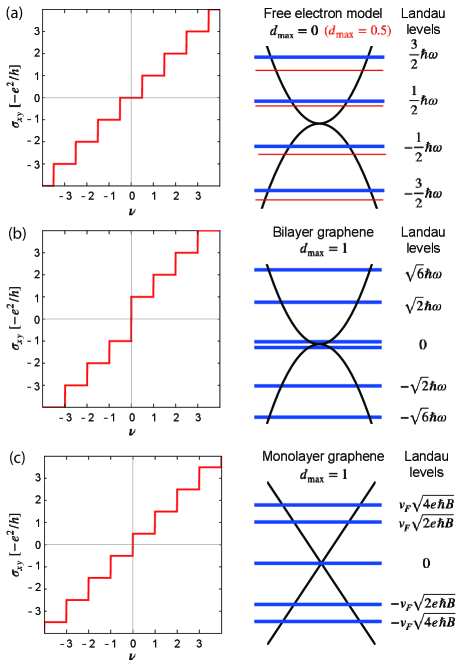
Graphene and its multilayer structures have garnered significant attention in various research fields, partly because of their unique carrier dynamics, sensitively dependent on the layer numbers [1, 2, 3, 4, 5, 6, 7, 8, 9, 10, 11, 12] . One notable example is the distinct quantum Hall effect (QHE) in monolayer and bilayer graphenes [13, 14, 15]. In monolayer graphene with linear band touching points, the carriers with pseudo-relativistic dispersion result in the half-integral quantum Hall plateaus characterized by the unique Landau Level spectrum with the energy $\epsilon^{\mathrm{single}}_{N}=\pm v_{F}\sqrt{2e\hbar B|N|}$, where $v_{F}$ is the Fermi velocity [13, 14, 15], $N$ is an integer, $B$ is a magnetic field, and $e$, $m$ are the electron’s charge and mass, respectively. This unique behavior arises from the $\pi$ Berry’s phase of the Dirac points.

On the other hand, in Bernal stacked bilayer graphene, simply bilayer graphene hereafter, the charge carriers exhibit a parabolic dispersion $\epsilon(p)=\pm\frac{p^{2}}{2m}$ with the effective mass $m$, hosting the Landau levels $\epsilon^{\mathrm{bilayer}}_{N}=\pm\hbar\omega\sqrt{N(N-1)}$. In bilayer graphene, the zero energy Hall plateau is absent, which is attributed to the $2\pi$ Berry phase around the quadratic band crossing point [15, 16]. It is noteworthy that although the parabolic band dispersion of the bilayer graphene is identical to that of the free electron gas, these two systems display entirely different Landau levels and QHEs. This indicates the importance of considering not only the band dispersion but also the geometry of wave functions to correctly describe the magnetic responses. The distinct Landau levels and QHEs of monolayer and bilayer graphenes are compared in Figure 1, in which we also plot the free electron gas Landau levels $\epsilon^{\mathrm{conv}}_{N}=\pm\hbar\omega(N+\frac{1}{2})$ with the cyclotron frequency $\omega=eB/m$ [17, 18].

Recent studies have shown that the quantum distance is a central quantity characterizing the geometric properties of two-dimensional quadratic band touching systems, leading to intriguing phenomena such as anomalous Landau level spreading [19, 20] and the emergence of boundary modes in flat band systems [21, 22]. More explicitly, the Hilbert-Schmidt quantum distance, or simply quantum distance, in momentum space is defined as

where $n$ is a band index and $\psi_{n,\bm{k}}$ is the Bloch eigenstate of the $n$-th band with crystal momentum $\bm{k}$. In particular, it was shown that the maximum quantum distance, denoted as $d_{\mathrm{max}}$, determines various geometric properties of the quadratic band crossing semimetals, including the Berry’s phase [23, 24]. In terms of $d_{\mathrm{max}}$, the geometry of bilayer graphene is characterized by $d_{\mathrm{max}}=1$, while the free electron with a quadratic band crossing is described by $d_{\mathrm{max}}=0$, indicating geometric triviality. Although these two systems have two distinct $d_{\mathrm{max}}$ values, to properly understand the role of the interband coupling in their distinct magnetic responses, one can design a model Hamiltonian that has fixed isotropic quadratic band dispersion $\epsilon(p)=\pm\frac{p^{2}}{2m}$ but with tunable quantum geometry.

In this paper, we examine the Landau levels, QHE, and magnetic response functions of the geometrically generalized model. By thoroughly examining them, we illustrate the nontrivial role of the interband coupling measured by $d_{\mathrm{max}}$ in magnetic responses of quadratic band crossing semimetals.

The rest of the paper is organized as follows. In Sec. II, we construct a model Hamiltonian for isotropic quadratic band touching semimetals, where the band dispersion remains $\pm p^{2}/(2m)$ while the geometry of wave functions is tunable. In Sec. III, we analyze the Landau levels of the model and examines the role of wave function geometry. In Sec. IV, we investigate the evolution of QHE between free electron gas and bilayer graphene. In Sec. V, we further explore the influence of wave function geometry on magnetic response functions using the Roth-Gaou-Niu relation [25, 26, 27]. Our concluding remarks can be found in Sec. VI. Appendixes contains the detailed calculations of Landau levels and a lattice model analysis.

Let us construct a general Hamiltonian whose energy eigenvalues are given by

Explicitly, we consider the Hamiltonian

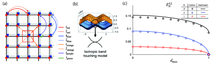
where $\sigma_{\alpha}$ represents an identity ($\alpha=0$) and Pauli matrices ($\alpha=x,y,z$), respectively. $h_{x,y,z}({\bm{k}})$ are real quadratic functions given by $h_{z}({\bm{k}})={-d\sqrt{1-d^{2}}}k_{y}^{2},~{}h_{y}({\bm{k}})=dk_{x}k_{y},~{}h_{x}({\bm{k}})=k_{x}^{2}/2+(1-2d^{2})k_{y}^{2}/2$, and $h_{0}({\bm{k}})=0$. Here, the parameter $d$ is defined as $d=\xi d_{\mathrm{max}}$ in which $\xi=\pm 1$, and $d_{\mathrm{max}}$ is the maximum value of the quantum distance $d_{\mathrm{HS},n}(\bm{k,k^{\prime}})$ between all the possible pairs of wave functions at $\mathbf{k}$ and $\mathbf{k}^{\prime}$ with the given band index $n=1,~{}2$. The energy eigenvalues of $\mathcal{H}_{0}({\bm{k}})$ remain unchanged from Eq. (2) regardless of the value of $d$ within the range $-1\leq d\leq 1$. When $d_{\mathrm{max}}=1$, the Hamiltonian in Eq. (3) corresponds to the low energy Hamiltonian of the Bernal stacked bilayer graphene [28, 29], and $\xi=\pm 1$ is related to the valley index. The parameters $d_{\mathrm{max}}$ and $\xi$ determine the Berry phase $\Phi_{B}$ [23] and quantum geometric tensor $g_{ij}^{n}$ given by $g_{ij}^{n}=2\braket{\partial_{k_{i}}u_{n}(\bm{k})}{\partial_{k_{j}}u_{n}(\bm{k})}-2\braket{\partial_{k_{i}}u_{n}(\bm{k})}{u_{n}(\bm{k})}\braket{u_{n}(\bm{k})}{\partial_{k_{j}}u_{n}(\bm{k})}$, where $u_{n}(\bm{k})$ is the $n$-th Bloch wave function [30]. Explicitly, for $\mathcal{H}_{0}({\bm{k}})$, the Berry phase and components of the quantum geometric tensor are given by

We note that more general quadratic band touching Hamiltonians, which exhibit anisotropic energy dispersions, require other geometric quantities to describe all possible interband coupling terms [24]. However, when the system has rotational symmetry, a single geometric parameter $d_{\mathrm{max}}$ suffices to fully characterize the quantum geometry [23, 24].

To understand the evolution of the Landau levels between $\epsilon_{N}^{conv}$ [Fig. 1(a)] and $\epsilon_{N}^{bilayer}$ [Fig. 1(b)], we introduce a perpendicular magnetic field $B$ to the Hamiltonian in Eq. (3). We consider the Landau gauge $\bm{A}=(0,Bx)$, which preserves translational invariance in the $y$-direction, and replace the momentum by ladder operators as $k_{x}\to(a+a^{\dagger})/(\sqrt{2}l_{B})$ and $k_{y}\to i(a-a^{\dagger})/(\sqrt{2}l_{B})$, where $l_{B}=\sqrt{\hbar/eB}$ is the magnetic length, and $a$($a^{\dagger}$) is the annihilation (creation) operator. To ensure the Hamiltonian’s hermiticity, we perform symmetrization: $k_{x}k_{y}=(k_{x}k_{y}+k_{y}k_{x})/2=i(a^{2}-(a^{\dagger})^{2})/(2l_{B}^{2})$. Then, the Hamiltonian reads

where $g_{11}=-g_{22}=d\sqrt{1-d^{2}}(2a^{\dagger}a+1-a^{\dagger 2}-a^{2})$ and $g_{12}=g_{21}^{\dagger}=-(2a^{\dagger}a+1)+(a^{2}-a^{\dagger 2})d+(2a^{\dagger}a+1-a^{2}-a^{\dagger 2})d^{2}$. It can be verified that when $d_{\mathrm{max}}=1$, this Hamiltonian corresponds to the low-energy effective Hamiltonian of bilayer graphene [29, 31]. In contrast, when $d_{\mathrm{max}}=0$, it corresponds to the conventional Hamiltonian, where electrons follow cyclotron orbits with the conventional Landau levels $\epsilon^{\mathrm{conv}}_{N}=\pm\hbar\omega(N+\frac{1}{2})$ [32]. The case where $d_{\mathrm{max}}$ is not an integer has not yet been explored. By investigating the regime $0<d_{\mathrm{max}}<1$, one can study how the magnetic properties of the conventional model gradually evolve into those of bilayer graphene.

Solving the transformed Hamiltonian yields the Landau levels (see Appendix for details):

where $N=\pm 2,\pm 3,...$ and $\mathrm{sgn}(N)$ represents the sign of $N$.

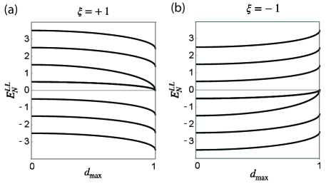
In Figure 2, the $d_{\mathrm{max}}$-dependence of Landau levels is depicted. When $d_{\mathrm{max}}=0$, the Landau levels $E^{LL}_{N}$ are equivalent to $\epsilon_{N}^{conv}$ but start to deviate from $\epsilon_{N}^{conv}$ as $d_{\mathrm{max}}$ increases. When $d_{\mathrm{max}}$ reaches one, they become $\epsilon_{N}^{bilayer}$. The degeneracy of Landau levels between $E^{LL}_{0}(d_{\mathrm{max}}=1)$ and $E^{LL}_{1}(d_{\mathrm{max}}=1)$ leads to the absence of a zero energy plateau in QHE as described in Section IV. Since such degeneracy of Landau levels occurs only when $d_{\mathrm{max}}=1$, the absence of the zero energy plateau cannot be observed if $d_{\mathrm{max}}\neq 1$.

One can verify that the degeneracy at $d_{\mathrm{max}}=1$ exists for both $\xi=\pm 1$. However, depending on $\xi$, the origin of zero Landau levels is different. For $\xi=+1$, the two zero energy levels come from the upper band, while for $\xi=-1$, the two zero energy levels come from the lower band. In a previous work [33], this $\xi$-dependence of zero energy Landau levels was demonstrated by creating a gap between two bands in bilayer graphene. Here, on the other hand, we verify that the $\xi$-dependence of zero energy Landau levels by continuously varying the quantum distance.

Furthermore, when $d_{\mathrm{max}}=1$ or $d_{\mathrm{max}}=0$, the Landau levels are symmetric with respect to $E=0$, as shown in Figs. 2(a) and (b). This result arises from chiral symmetry, represented by the operator $\sigma_{z}$, which satisfies $\sigma_{z}H_{0}(\bm{k})\sigma_{z}=-H_{0}(\bm{k})$, exclusively when $d_{\mathrm{max}}=1$ or $d_{\mathrm{max}}=0$. This symmetry holds even in the presence of a magnetic field (See Appendix). In fact, the chiral symmetry is crucial for the degeneracy observed at $d_{\mathrm{max}}=1$. To confirm this idea, we introduce a perturbation $H_{\text{pert}}=\delta k^{2}\sigma_{0}$ that breaks the chiral symmetry, and subsequently calculate the resulting Landau levels. With this perturbation, the zeroth and first Landau levels for $d_{\mathrm{max}}=1$ shift to $E^{LL}_{0}=\frac{\xi}{2}\hbar\omega\delta$ and $E^{LL}_{1}=\frac{3\xi}{2}\hbar\omega\delta$, respectively, thereby lifting the degeneracy. This demonstrates that the presence of the zero energy plateau necessitates chiral symmetry as well as $d_{\mathrm{max}}=1$.

In addition, when the Hamiltonian possessses chiral symmetry, one can define a winding number ($W$):

Explicitly, for $d_{\mathrm{max}}=0$ and $d_{\mathrm{max}}=1$, we obtain

This indicates that the presence of the zero energy plateau is contingent upon chiral symmetry with a winding number of two.

For $0<d_{\mathrm{max}}<1$, the chiral symmetry is broken because the Hamiltonian in Eq. (3) has nonzero $h_{x}$, $h_{y}$ and $h_{z}$, simultaneously. Consequently, the Landau levels are no longer symmetric with respect to $E=0$. However, one can still find the symmetry between $\xi=+1$ and $\xi=-1$ cases in which the Landau levels have the opposite signs, as shown in Eq. (7), Figs. 2(a) and (b). For $|N|\gg 1$, this can be understood using the semiclassical results given by [26]

where $\Phi_{B}$ is Berry phase. For both $\xi=\pm 1$ cases with $|N|\gg 1$, the Landau levels in Eq. (7) are identical to those in Eq. (10). Depending on $\xi$, the sign of $\Phi_{B}$ changes oppositely, as shown in Eq. (33), explaining the symmetric structure of the Landau levels between $\xi=+1$ and $\xi=-1$ cases. Interestingly, this symmetric structure persists even for low $N$ as explicitly shown in Eq. (7).

The dependence of the Landau levels on $d_{\mathrm{max}}$ significantly influences the QHE. Here, we focus on the case $\xi=+1$; the results for $\xi=-1$ can be obtained by reversing the sign of the energies for $\xi=1$ as shown in Fig. 2. To understand the influence of $d_{\mathrm{max}}$ on QHE, it is more insightful to examine the magnetic field dependence of Hall conductivity or Hall resistivity rather than the filling factor dependence of Hall conductivity. This is because the continuous variation from $d_{\mathrm{max}}=0$ to $d_{\mathrm{max}}=1$ is not apparent in the latter case; instead, a sudden change is observed at $d_{\mathrm{max}}=1$ due to the zero energy degeneracy. Therefore, we analyze the magnetic field dependence of QHE by varying $d_{\mathrm{max}}$ when the electron density is fixed.

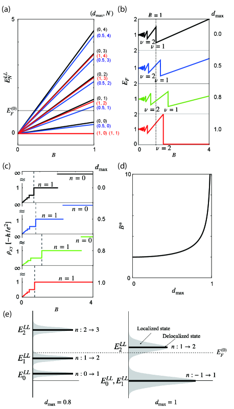
Figure 3(a) shows the magnetic field dependence of the Landau levels in Eq. (7). As the magnetic field increases, the topmost occupied level changes when the filling factor $\nu$ reaches integer values. At theses points, $E_{F}$ transitions from $E^{LL}_{\nu}$ to $E^{LL}_{\nu-1}$. Figure 3(b) shows the magnetic field dependence of the Fermi energy $E_{F}(B)$, referred to as Shubnikov-de Hass oscillation, for various values of $d_{\mathrm{max}}=0,0.5,0.8$ and 1. Increasing $d_{\mathrm{max}}$ shifts the magnetic field $B_{\nu=i}$ where the transition occurs with an integer $i$. Furthermore, the slope of the Fermi energy at $B_{\nu=i}$, defined as

decreases with higher values of $d_{\mathrm{max}}$. Specifically,

More generally, $m_{i}=E_{i-1}^{LL}/B$. The decrease in the slopes $m_{1}$ and $m_{2}$ with increasing $d_{\mathrm{max}}$ causes $B_{1}$, where the $E_{F}$ transitions from $E^{LL}_{1}$ to $E^{LL}_{0}$, to increase. When $d_{\mathrm{max}}$ reaches one, these slopes approach zero, making $B_{1}$ infinite. This implies that the first Landau level $E^{LL}_{1}$ is always occupied when $E_{F}^{(0)}>0$ where $E_{F}^{(0)}$ is the Fermi level at zero magnetic field.

To consider Hall plateaus, we assume the disorder induced Landau level broadening as schematically illustrated in Figure 3(e) where delocalized electrons exist in the middle of each level while the rest of the states are localized. The Hall resistivity $\rho_{xy}$ is quantized as $\rho_{xy}=-h/(ne^{2})$ with a natural number $n$. More explicitly, $n$ is determined by $n=N+1-\delta_{d_{\mathrm{max}},1}$, where $N$ is the largest integer that satisfies $E^{(0)}>E^{LL}_{N}$. Figure 3(c) shows the magnetic field dependence of Hall resistivity for $d_{\mathrm{max}}=0,0.5,0.8$ and 1. Similar to the oscillating $E_{F}$, the magnetic field at which $\rho_{xy}$ jumps strongly depends on $d_{\mathrm{max}}$. Increasing $d_{\mathrm{max}}$ extends the length of $n=1$ plateau and shifts the magnetic field $B^{*}$ where the transition from $n=1$ plateau to $n=0$ plateau occurs. Figure 3(d) shows the $d_{\mathrm{max}}$ dependence of $B^{*}$. When $d_{\mathrm{max}}=1$, $B^{*}$ becomes infinity, indicating that the $n=0$ plateau does not exist.

Furthermore, as shown in the dashed vertical lines in Fig. 3(c), one can observe that the jump between $n=1$ and $n=2$ plateaus occurs at higher magnetic fields as $d_{\mathrm{max}}$ increases when $0\leq d_{\mathrm{max}}<1$. However, when $d_{\mathrm{max}}=1$, this jump suddenly occurs at a relatively lower magnetic field. This phenomenon originates from the chiral symmetry and the degeneracy between the zeroth and first Landau levels in Eq. (7).

More explicitly, the Hall resistivity changes when the Fermi energy passes the delocalized state, as shown in Fig. 3(e). For $d_{\mathrm{max}}<1$, the transition between the $n=1$ and $n=2$ plateaus occurs when $E_{F}^{(0)}=E_{1}^{LL}$. Since $E_{1}^{LL}(d_{\mathrm{max}})=\frac{3\hbar e}{2m}B\sqrt{1-d_{\mathrm{max}}^{2}}$, the jump requires a higher $B$ as $d_{\mathrm{max}}$ increases. On the other hand, at $d_{\mathrm{max}}=1$, the transition between the $n=1$ and $n=2$ plateaus happens when $E_{F}^{(0)}=E_{2}^{LL}=\frac{\hbar e}{m}\sqrt{2}B$. This is because filling $E_{0}^{LL}$ and $E_{1}^{LL}$ corresponds to the jump between $n=-1$ and $n=+1$ plateaus due to chiral symmetry. Note that the system is electrically neutral when both $E^{LL}_{0}$ and $E^{LL}_{1}$ are half-filled. Therefore, the transition between $n=1$ and $n=2$ plateaus occurs when $E_{F}^{(0)}=E_{2}^{LL}(d_{\mathrm{max}}=1)$, while for $d_{\mathrm{max}}<1$ it occurs when $E_{F}^{(0)}=E_{1}^{LL}$ [Fig. 3(e)]. Consequently, the jump between $n=1$ and $n=2$ plateaus for $d_{\mathrm{max}}=1$ does not follow the trend observed when $d_{\mathrm{max}}<1$.

Magnetic response functions also exhibit strong dependence on $d_{\mathrm{max}}$. We explore how $d_{\mathrm{max}}$ influences magnetic response functions by utilizing the Roth-Gaou-Niu relation [25, 26, 27] given by

where $N_{0}(\epsilon_{F})$ is the zero-field integrated density of states at the Fermi energy $\epsilon_{F}$ (i.e., $N^{\prime}_{0}=\partial_{\epsilon}N_{0}$ is the density of states), $M_{0}(\epsilon_{F})$ is the spontaneous magnetization, and $\chi_{0}(\epsilon_{F})$ is the magnetic susceptibility. Here, the prime denotes the derivative with respect to the energy: $M^{\prime}_{0}=\partial_{\epsilon}M_{0}$, $\chi^{\prime}_{0}=\partial_{\epsilon}\chi_{0}(\epsilon)$. These quantities, which depend on the Fermi energy $\epsilon_{F}$, are evaluated at zero temperature and in the limit of zero magnetic field. Below, we adopt units where $\hbar=1$ and the flux quantum $\phi_{0}=h/e=1$.

By applying the results in Eq. (7) to Eq. (14), we obtain the following expressions ¹¹1Solve $E_{N}^{LL}=\epsilon_{F}$ for N, then we get the results.

We note that the integrated density of states $N_{0}(\epsilon_{F})$ solely depends on $\epsilon_{F}$ independent of $d_{\mathrm{max}}$ because $d_{\mathrm{max}}$ does not contribute to the energy dispersion.

The fact that the derivative of $M_{0}$ is proportional to the Berry phase indicates that the average of the orbital magnetic moment over the Fermi surface vanishes, i.e., $\braket{\mathcal{M}}_{\epsilon_{F}}=0$. This is because, according to the modern theory of magnetization [35, 27, 36], differentiating the magnetization with respect to the chemical potential gives

where $\braket{\mathcal{M}}_{\epsilon_{F}}$ represents the average of the orbital magnetic moment over the Fermi surface. Indeed, for a two-band model with electron-hole symmetry, the orbital magnetic moment is directly related to the Berry curvature: $\mathcal{M}(\bm{k})=\frac{e}{\hbar}\epsilon_{+}(\bm{k})\Omega(\bm{k})$, where $\Omega$ is the Berry curvature [37, 38]. In a quadratic band touching semimetal, the Berry curvature at finite $\bm{k}$ is always zero while the Berry phase $\Phi_{B}(d_{\mathrm{max}})$ can be finite [23]. Therefore, the average of the orbital magnetic moment over the Fermi surface vanishes, and $M^{\prime}_{0}(\epsilon_{F})=\frac{\Phi_{B}(d_{\mathrm{max}})}{2\pi}$.

The result for the derivative of the susceptibility agrees with the known results for free electron model and bilayer graphene when $d_{\mathrm{max}}=0$ and $d_{\mathrm{max}}=1$, respectively [27, 39, 28]. Considering the form of the susceptibility in the free electron model and bilayer graphene as well as Eq. (17) ²²2The susceptibility is given $\chi_{0}(\epsilon_{F})=\frac{\pi}{6}$ for free electrons and $\chi_{0}(\epsilon_{F})=\frac{\pi}{2}(\frac{1}{3}+\ln{\frac{|\epsilon_{F}|}{t}})$ for bilayer graphene[27, 39, 28]. The derivative of the susceptibility is $\chi’_{0}(\epsilon_{F})=d_{\mathrm{max}}^{2}\frac{\pi}{2\epsilon_{F}}$ from Eq. (17)., we propose the following expression for the susceptibility:

where $t$ is a constant. For bilayer graphene, the constant $t$ is related to interlayer hopping [28, 39]. One can verify that the derivative of the above equation gives Eq. (17).

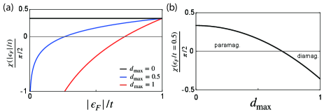
Furthermore, it can be observed that the sign of $\chi$ changes when $|\epsilon_{F}|<t$, as shown in Fig. 4, at the critical value

When $d_{\mathrm{max}}>d_{\mathrm{max,c}}$, the system exhibits paramagnetism, i.e., $\chi_{0}>0$. On the other hand, when $0<d_{\mathrm{max}}<d_{\mathrm{max,c}}$, the system exhibits diamagnetism, i.e., $\chi_{0}<0$. The sign change in $\chi_{0}$ as $d_{\mathrm{max}}$ varies indicates that a change in geometry alone, without altering the band structure or Fermi level, can induce a magnetic phase transition.

To summarize, we have studied the influence of $d_{\mathrm{max}}$ on Landau levels, the QHE, and magnetic response functions of isotropic quadratic band-touching systems. Despite sharing the same energy dispersion, distinct wave function geometry, characterized by different $d_{\mathrm{max}}$, gives rise to markedly different Landau levels, QHE, and magnetic response functions. To experimentally observe how these physical properties evolve with changes in $d_{\mathrm{max}}$, it is crucial to identify systems where tuning $d_{\mathrm{max}}$ is feasible. Achieving a non-integer $d_{\mathrm{max}}$ in momentum space requires $h_{x}(\bm{k}),h_{y}(\bm{k}),h_{z}(\bm{k})\neq 0$ in the Hamiltonian in the Eq. (3) simultaneously. This indicates imaginary and long-range (at least the next nearest neighboring ones) hoppings are necessary in real space, suggesting that materials with strong spin-orbit coupling could be potential candidates for $0<d_{\mathrm{max}}<1$. Our finding underscores the significance of quantum geometry of wavefunctions on the magnetic properties of electronic systems. Considering the growing interest in the physical responses induced by the quantum geometry, revealing the relation between physical responses and geometry in more general multi-band semimetal systems is an important direction for future study.