Revisiting Kepler: new symmetries of an old problem

Gil Bor¹¹1 CIMAT, A.P. 402, Guanajuato, Gto. 36000, Mexico; [email protected] Connor Jackman²²2 CIMAT, A.P. 402, Guanajuato, Gto. 36000, Mexico; [email protected]

Abstract

The Kepler orbits form a 3-parameter family of unparametrized plane curves, consisting of all conics sharing a focus at a fixed point. We study the geometry and symmetry properties of this family, as well as natural 2-parameter subfamilies, such as those of fixed energy or angular momentum.

Our main result is that Kepler orbits is a ‘flat’ family, that is, the local diffeomorphisms of the plane preserving this family form a 7-dimensional local group, the maximum dimension possible for the symmetry group of a 3-parameter family of plane curves. These symmetries are different from the well-studied ‘hidden’ symmetries of the Kepler problem, acting on energy levels in the 4-dimensional phase space of the Kepler system.

Each 2-parameter subfamily of Kepler orbits with fixed non-zero energy (Kepler ellipses or hyperbolas with fixed length of major axis) admits $\mathrm{PSL}_{2}(\mathbb{R})$ as its (local) symmetry group, corresponding to one of the items of a classification due to A. Tresse (1896) of 2-parameter families of plane curves admitting a 3-dimensional local group of symmetries. The 2-parameter subfamilies with zero energy (Kepler parabolas) or fixed non-zero angular momentum are flat (locally diffeomorphic to the family of straight lines).

These results can be proved using techniques developed in the 19th century by S. Lie to determine ‘infinitesimal point symmetries’ of ODEs, but our proofs are much simpler, using a projective geometric model for the Kepler orbits (plane sections of a cone in projective 3-space). In this projective model all symmetry groups act globally.

Another advantage of the projective model is a duality between Kepler’s plane and Minkowski’s 3-space parametrizing the space of Kepler orbits. We use this duality to deduce several results on the Kepler system, old and new.

1 Introduction and statement of main results

A Kepler orbit is a plane conic – ellipse, parabola or hyperbola – with a focus at the origin (in case of a hyperbola only the branch bending around the origin is taken). Kepler orbits form a 3-parameter family of plane curves, traced by the motions of a point mass subject to Newton’s inverse square law: the radial attractive force is proportional to the inverse square of the distance to the origin. We exclude ‘collision orbits’ (lines through the origin). See Figure 1.

Refer to caption — Figure 1: Kepler orbit types (ellipse, parabola or hyperbola), shapes and sizes are given by their energy $E$ and angular momentum $M$ . The major axis is $1/|E|$ and the Latus rectum (vertical dotted segment) is $2M^{2}$ . See Section 3.

1.1 Orbital symmetries

These are local diffeomorphisms of $\mathbb{R}^{2}\setminus 0,$ taking (unparametrized) Kepler orbits to Kepler orbits. At the outset, it is not clear that there are any such symmetries, local or global, other than the obvious ones – dilations and rotations about the origin, or reflections about lines through the origin (a 2-dimensional group of symmetries). Nevertheless, as we find out, there are many additional orbital symmetries, both for the full 3-parameter family of Kepler orbits, as well as for some natural 2-parameter subfamilies.

Theorem 1.

The orbital symmetries of the Kepler problem form a 7-dimensional group of local diffeomorphisms of $\mathbb{R}^{2}\setminus 0$ (aka a ‘pseudo-group’), the maximum dimension possible for a 3-parameter family of plane curves, generated by the following infinitesimal symmetries (vector fields whose flows act by orbital symmetries):

r\partial_{r},\ \partial_{\theta},\ r\partial_{x},\ r\partial_{y},\ -xr\partial_{r},\ -yr\partial_{r},\ -r^{2}\partial_{r}

(1)

(using both Cartesian and polar coordinates).

Note that the first two vector fields generate dilations and rotations, the ‘obvious’ symmetries mentioned above. How about the rest of the symmetries? Where do they come from?

We emphasis that the 7 vector fields of Theorem 1 do not generate a honest 7-dimensional Lie group action on $\mathbb{R}^{2}\setminus 0$ . The first 4 vector fields do generate an action of the connected component of the group $\mathrm{CO}_{2,1}$ on $\mathbb{R}^{2}\setminus 0$ , but the last three vector fields are in fact imcomplete (their integral curves “run to infinity” in finite time). As we explain later, to obtain a global group action, one needs to embedd the Kepler plane in a larger surface, a cone in $\mathbb{R}P^{3}$ , to which the above 7 vector fields extend, generating an action of the 7-dimensional subgroup of $\mathrm{PGL}_{4}(\mathbb{R})$ preserving this cone.

Now quite generally, there is a standard method for finding infinitesimal symmetries of $n$ -parameter families of plane curves, going back to S. Lie in the 19th century, consisting of first writing down an $n$ -th order scalar ODE whose graphs of solutions form the curves of the family. Then, one writes down a system of PDEs for the infinitesimal symmetries of this ODE, which with some luck and skill, one can solve explicitly. See Chapter 6 of P. Olver’s book [37]. This is a straightforward albeit tedious procedure (best left nowadays to computers), producing the infinitesimal symmetries above, but the result remains mysterious.

Instead, our proof of Theorem 1 exploits the peculiar geometry of Kepler’s problem, in particular, its projective geometry, borrowing from Lie’s theory only the upper bound of 7 on the dimension of the symmetry group. This proof, rather then the actual statement of Theorem 1, is the main thrust of this article. See subsection 1.3 below for a sketch of the proof.

1.2 The space of Kepler orbits

As is well known, every Kepler orbit is the orthogonal projection onto the $xy$ plane (the ‘Kepler plane’) of a conic section, the intersection of the cone $\mathcal{C}:=\{x^{2}+y^{2}=z^{2}\}\subset\mathbb{R}^{3}$ with a plane $ax+by+cz=1,\ c\neq 0$ . See Section 3 below for a proof (due to Lagrange [30]) as well as a reminder of some other standard facts about the Kepler problem. Let $\mathbb{R}^{2,1}$ be the 3-dimensional space with coordinates $(a,b,c)$ equipped with Minkowski’s quadratic form $\|(a,b,c)\|^{2}:=a^{2}+b^{2}-c^{2}$ (we use this notation even though the expression has negative values!). Note that the planes $ax+by+cz=1$ and $ax+by-cz=1$ (the reflection of the former about the $xy$ plane) generate the same Kepler orbit. Thus $\mathbb{R}^{2,1}_{+}=\{c>0\}\subset\mathbb{R}^{2,1}$ is identified with the space of Kepler orbits. Furthermore, the cone $\|(a,b,c)\|^{2}=0$ parametrizes Kepler parabolas, its interior $\|(a,b,c)\|^{2}<0$ parametrizes Kepler ellipses and its exterior $\|(a,b,c)\|^{2}>0$ parametrizes Kepler hyperbolas. See Figure 2.

The orbital symmetries of Theorem 1 clearly act on the space of Kepler orbits and thus on $\mathbb{R}^{2,1}_{+}$ . Again, this is only a local action (a 7-dimensional Lie algebra of vector fields), but it extends to a global action on all of $\mathbb{R}^{2,1}$ .

Theorem 2.

The local group action of the orbital symmetries of the Kepler problem on $\mathbb{R}^{2,1}_{+}$ extends to $\mathbb{R}^{2,1}$ , generating the identity component of the group $\mathrm{CO}_{2,1}\ltimes\mathbb{R}^{2,1}$ of Minkowski similarities (compositions of Minkowski rotations, dilations and translations). The infinitesimal generators of this action, corresponding to those of Equation (1), are

-a\partial_{a}-b\partial_{b}-c\partial_{c},\ -b\partial_{a}+a\partial_{b},\ -a\partial_{c}-c\partial_{a},\ -b\partial_{c}-c\partial_{b},\ \partial_{a},\ \partial_{b}\ ,\partial_{c}.

(2)

The first vector field generates dilations in $\mathbb{R}^{2,1}$ , the next 3 generate Minkowski rotations about the origin and the last 3 generate translations. It follows that orbital symmetries actually ‘mix’ the orbit types (ellipses, parabolas, hyperbolas).

The horizontal plane $\{c=0\}\subset\mathbb{R}^{2,1}$ corresponds to ‘ideal’ Kepler orbits which are inevitably added upon completing the orbital symmetry action. For $(a,b,0)\neq(0,0,0)$ they are (affine) lines in $\mathbb{R}^{2}\setminus 0$ , obtained by projecting to the $xy$ plane sections of $\mathcal{C}$ by vertical affine 2-planes in $\mathbb{R}^{3}$ . The point $(0,0,0)\in\mathbb{R}^{2,1}$ corresponds to the ‘line at infinity’ in the Kepler plane.

1.3 Sketch of proof of Theorems 1 and 2

With Figure 2 in mind, consider the group $\mathrm{CO}_{2,1}\subset\mathrm{GL}_{3}(\mathbb{R})$ , preserving the quadratic form $x^{2}+y^{2}-z^{2}$ up to scale. Its identity component acts on $\mathcal{C}_{+}:=\{x^{2}+y^{2}=z^{2},z>0\}$ , preserving its set of plane sections, thus projects to an action on $\mathbb{R}^{2}\setminus 0$ by orbital symmetries. This accounts for the first 4 vector fields of Equation (1).

Next, consider the 3-dimensional projective space $\mathbb{R}P^{3}$ with homogeneous coordinates $(X:Y:Z:W)$ and embed $\mathbb{R}^{3}\hookrightarrow\mathbb{R}P^{3}$ as the affine chart $W\neq 0$ , $(x,y,z)\mapsto(x:y:z:1).$ The closure of $\mathcal{C}$ in $\mathbb{R}P^{3}$ , $\overline{\mathcal{C}}=\{(X:Y:Z:W)\,|\,X^{2}+Y^{2}=Z^{2}\}$ , is obtained by adding to $\mathcal{C}$ the ‘circle at infinity’ $S^{1}_{\infty}=\{X^{2}+Y^{2}=Z^{2},W=0\}$ . See Figure 3. Now consider the group $\widetilde{\mathcal{G}}\subset\mathrm{GL}_{4}(\mathbb{R})$ , preserving the (degenerate) quadratic form $X^{2}+Y^{2}-Z^{2}$ , up to scale. A simple calculation (see Section 5 below) shows that $\widetilde{\mathcal{G}}$ is an 8-dimensional group, thus its image $\mathcal{G}=\widetilde{\mathcal{G}}/\mathbb{R}^{*}\subset\mathrm{PGL}_{4}(\mathbb{R})$ is $7$ -dimensional, acting effectively on $\overline{\mathcal{C}}$ , preserving its set of (projective) plane sections. It leaves invariant the set of sections by planes not passing through the vertex of $\overline{\mathcal{C}}$ , parametrized by $\mathbb{R}^{2,1}$ . The action restricts to a local action on $\mathcal{C}_{+}\subset\overline{\mathcal{C}}$ , then projects to a local action on $\mathbb{R}^{2}\setminus 0$ by orbital symmetries. Equations (1) and (2) follow easily from this description.

Finally, we use a basic result of Lie’s theory of symmetries of ODEs (reviewed in the Appendix), according to which the maximum dimension of the group of point symmetries of a 3rd order ODE is 7, thus the above construction provides the full group of orbital symmetries of the Kepler problem. See Section 5 below for the full details.

1.4 2-parameter subfamilies

The simplest example of a 2-parameter family of plane curves (also called a ‘path geometry’) is the family of straight lines. It admits an 8-dimensional local group of symmetries (the projective group), the maximum dimension possible for a 2-parameter family of plane curves. A 2-parameter family of plane curves locally diffeomorphic to this family is called flat. There are no straight lines among Kepler orbits, but there are flat 2-parameter subfamilies.

Theorem 3.

Kepler’s parabolas form a flat 2-parameter family of curves. The map ${\mathbf{z}}\mapsto{\mathbf{z}}^{2}$ (in complex notation) is a local diffeomorphism taking straight affine lines to Kepler parabolas.

This theorem is essentially known. The squaring map ${\mathbf{z}}\mapsto{\mathbf{z}}^{2}$ , in the context of the Kepler problem, is known sometimes as the Levi-Civita or Bohlin map. It can be used to define a local orbital equivalence between Hooke and Kepler orbits (see e.g. Appendix 1 of [5]).

Theorem 4.

Kepler’s orbits with fixed angular momentum $\pm M\neq 0$ form a flat 2-parameter family of curves. The map ${\mathbf{r}}\mapsto{\mathbf{r}}/(1-r/M^{2})$ takes Kepler orbits with angular momentum $M$ to straight lines.

See Section 3 for a reminder about the angular momentum (also Figure 1). The proof of this theorem is particularly simple using the geometry of the space $\mathbb{R}^{2,1}$ of Kepler orbits: the family of Kepler orbits with fixed $|M|$ is represented in $\mathbb{R}^{2,1}$ by a horizontal plane; a vertical translation in this space, which according to Theorem 2 is available as an orbital symmetry, maps this plane to the plane $c=0$ , parametrizing lines in the $xy$ -plane.

Next we consider Kepler orbits with fixed energy $E\neq 0.$ These fill up a plane region $\mathcal{H}_{E}$ , the Hill region. For $E\geq 0$ (Kepler hyperbolas with major axis $1/E$ or Kepler parabolas) the Hill region is the whole punctured plane, for $E<0$ (Kepler ellipses with major axis $1/|E|$ ) it is a punctured disk of radius $1/|E|$ . See Figure 4.

Theorem 5.

$(\mathrm{a})$

For each fixed energy $E\neq 0$ , the 2-parameter family of Kepler orbits with energy $E$ is non flat but is locally homogeneous: its orbital symmetry group is a 3-dimensional subgroup of the 7-dimensional group of Kepler’s orbital symmetries, isomorphic to $\mathrm{PSL}_{2}(\mathbb{R})$ and generated by the infinitesimal symmetries

$\partial_{\theta},r(\partial_{x}+Ex\partial_{r}),r(\partial_{y}+Ey\partial_{r}).$ (3)
$(\mathrm{b})$

For $E<0$ the action of $\mathrm{PSL}_{2}(\mathbb{R})$ on the Hill region $\mathcal{H}_{E}$ is global; for $E>0$ it is only local.

This theorem is also essentially known, or at least can be deduced easily by experts on ‘superintegrable metrics’ from known results from the 19th centrury by S. Lie and G. Koenigs (see for example [14] and references within; we thank V. Matveev for pointing out to us this relation).

Our proof of this theorem is quite simple using the geometry of the space of orbits $\mathbb{R}^{2,1}$ : as we explain in Section 3, orbits of fixed energy $E$ correspond to one of the sheets of the hyperboloid of two sheets $a^{2}+b^{2}-(c-|E|)^{2}=-E^{2}$ (the upper sheet for $E<0$ , the lower one for $E>0$ ). See Figure 5(iii). The Minkowski metric in $\mathbb{R}^{2,1}$ restricts to a hyperbolic metric in each of these sheets, the subgroup of $\mathcal{G}\simeq\mathrm{CO}_{2,1}\ltimes\mathbb{R}^{2,1}$ preserving the hyperboloid acts as the full group of isometries of this metric, with generators given by Equation (3).

Any two Hill regions with the same sign of energy are obviously orbitally equivalent by dilation. For opposite signs of energies this is still true but less obvious.

Theorem 6.

$\mathcal{H}_{1}$ is orbitally embedded in $\mathcal{H}_{-1}$ by the map ${\mathbf{r}}\mapsto{\mathbf{r}}/(1+2r).$ See Figure 6.

Viewed in $\mathbb{R}^{2,1}$ , where the two Hill regions correspond to the two sheets of a hyperboloid, the map is simply the reflection about a horizontal plane $c=1$ , interchanging the two sheets. See Figure 5(iii).

1.5 Further results

1.

We establish a dictionary between the Minkowski geometry of the Kepler orbit space $\mathbb{R}^{2,1}$ and properties of Kepler orbits. For example: a parabolic (or isotropic) plane in $\mathbb{R}^{2,1}$ corresponds to the family of Kepler orbits passing through a fixed point. See Table 1 of Section 4.
2.

We give three illustrations of the usage of this dictionary: a new proof of ‘Kepler’s fireworks’ (Proposition 4.13), a Keplerian analogue of the 4 vertex and Tait-Kneser theorems (Theorem 8) and a ‘minor axis version’ of Lambert’s Theorem (Theorem 9).
3.

Similar results to Theorems 1-6 hold for orbital symmetries of the Hooke problem – the set of conics sharing a center (trajectories of mass points under central force proportional to the distance to the origin), and the orbits of the corresponding ‘Coulomb’ problems, where the sign of the force is reversed, becoming a repelling force. By central projection, our results extend to Hooke and Kepler orbits on surfaces of constant curvature (sphere and hyperbolic plane). See Table 2.
4.

We establish a converse to Theorem 1: among all central forces, Hooke and Kepler force laws are the only ones producing ‘flat’ families of orbits (3 parameter families with a 7-dimensional group of symmetries). See Theorem 10. This is reminiscent of Bertrand’s Theorem (1873), characterizing these two force laws as the only central force laws with bound orbits all of whose bound orbits are closed [9], [6, page 37].

* * *

Techniques. Other than standard projective and differential geometric constructions, we use some of the work of S. Lie (1874), A. Tresse (1896) and K. Wünschmann (1905) on point symmetries of 2nd and 3rd order ODEs. We do not assume the reader’s familiarity with their work. We summarize in the Appendix the needed tools of this theory.

Figures. The figures here were computer generated using Wolfram’s Mathematica and Apple’s Keynote.

Acknowledgment. We thank Richard Montgomery, Sergei Tabachnikov, Alain Albouy and Vladimir Matveev for fruitful correspondence and discussions. GB was supported by CONACYT Grant A1-S-4588.

2 Wider context: ‘orbital’ vs ‘dynamical’ symmetries

The Kepler problem is centuries old with an enormous literature. It is hard to imagine one can add anything new to this problem in the 21st century. Yet, new and interesting works continue to appear. See, for example, [8, 10, 35, 42, 23, 28]. Some facts have been rediscovered several times, centuries apart, especially before the existence of internet search engines. For example, V.I. Arnol’d attributes in his 1990 book [5, Appendix 1] the fact that ${\mathbf{z}}\mapsto{\mathbf{z}}^{2}$ maps Hooke orbits to Kepler orbits to K. Bohlin’s 1911 article [11], then goes on to generalize it to a ‘duality’ between central force power laws. In fact, all this appeared in C. Maclaurin’s 1742 ‘Treatise of fluxions’ [32, Book II, Chap. V, §875] (we thank S. Tabachnikov for pointing out this reference to us).

One of the most studied aspects of the Kepler problem are its symmetry properties. The most obvious symmetries are diffeomorphisms of the plane, mapping solutions ${\mathbf{r}}(t)$ of the underlying ODE, $\ddot{\mathbf{r}}=-{\mathbf{r}}/r^{3}$ , to solutions. One can show that these consist only of the rotations about the origin and reflections about lines through the origin, valid for any central force motion.

More interesting symmetries arise when the Kepler problem is considered as a Hamiltonian system, ie a flow defined on its phase space $T^{*}(\mathbb{R}^{2}\setminus 0)$ . The symplectomorphisms of phase space preserving parametrized trajectories of this flow form a larger group of symmetries, associated to the Hamiltonian flows of additional conserved quantities such as components of the Laplace-Runge-Lenz vector. These symmetries generate a (local) $\mathrm{SO}_{3}$ -action on the open subset of phase space with negative energy. Apart from the lift of the rotation symmetries above, these oft-called ‘hidden’ symmetries do not descend to an action on the Kepler plane, even locally. The action is rather on phase space, mixing position and momentum variables. A good reference for this type of ‘dynamic’ or ‘phase space’ symmetries of the Kepler problem is the book [28] or Chapters 3 and 4 of [22].

In contrast, the symmetries in this article are ‘orbital’ symmetries, acting on the configuration space of the Kepler problem, $\mathbb{R}^{2}\setminus 0$ , not its phase space. They are closer to the symmetries one can extract from Albouy’s ‘projective dynamics’ papers [1, 2].

So how original are our results? As far as we can tell, after consulting with experts and searching the literature, our results are new. The articles [1, 2, 15] are the nearest in spirit that we found. ‘Hidden symmetries’ of the Kepler problem, ie of its phase space, have been studied extensively, and symmetries of 2nd and 3rd order ODEs have been studied extensively as well since the mid 19th century, but it seems that the symmetries of the 2nd and 3rd order ODEs that arise in the Kepler problem have not been studied systematically before, which is the present article’s contribution.

But of course, given the subject’s long and rich history, it is is still quite possible that at least some of the theorems announced here have been noted before, in some form or another. If some of the readers of this article are aware of such work we will be grateful if they contact us.

3 A reminder on the Kepler problem

Here we review briefly some well known facts about the Kepler problem that will be used in the sequel. See also [3, 5, 6, 23].

Kepler orbits are the unparametrized plane curves traced by the solutions of the ODE

\ddot{\mathbf{r}}=-{{\mathbf{r}}\over r^{3}},

(4)

where ${\mathbf{r}}={\mathbf{r}}(t)=(x(t),y(t))\in\mathbb{R}^{2}\setminus 0$ and $r:=\|{\mathbf{r}}\|=\sqrt{x^{2}+y^{2}}.$

The energy and angular momentum of a solution are

E:={1\over 2}\|\dot{\mathbf{r}}\|^{2}-{1\over r},\quad M:=x\dot{y}-y\dot{x},

(5)

respectively, and can be easily shown to remain constant during the motion.

Note that $M$ is twice the sectorial velocity, the rate at which area is swept by the line segment connecting the origin to ${\mathbf{r}}(t)$ . It follows that $M=0$ if and only if the motion is along a line passing through the origin. Our exclusion of ‘collision’ orbits thus amounts to assuming $M\neq 0.$ Note also that although $E$ and $M$ are defined in equation (5) via the time parametrization of the Kepler orbit, they are in fact determined by the shape of the underlying unparametrized curve (except for the sign of $M$ ). See Figure 1.

A conic in a Euclidean plane is the locus of points with constant ratio of distances to a fixed point and a fixed line. The fixed point, line and ratio are called a focus, directrix and eccentricity $e$ (respectively). Conics with $e>1$ , $e=1$ , $0<e<1$ and $e=0$ are hyperbolas, parabolas, non-circular ellipses and circles (respectively).

Identify the $xy$ plane with the plane $z=0$ in $\mathbb{R}^{3}$ , $(x,y)\mapsto(x,y,0)$ . We use the term ‘projection’ to mean the orthogonal projection $\mathbb{R}^{3}\to\mathbb{R}^{2},$ $(x,y,z)\mapsto(x,y)$ .

Theorem 7.

$(\mathrm{a})$

Every Kepler orbit is the projection of a section of the cone $\mathcal{C}=\{x^{2}+y^{2}=z^{2}\}\subset\mathbb{R}^{3}$ by a plane $ax+by+cz=1$ , $c\neq 0.$

More precisely: if $c>0$ then the orbit is the projection of the intersection of the plane with the upper cone $\mathcal{C}_{+}:=\mathcal{C}\cap\{z>0\}$ ; if $c<0$ then it is the projection of the intersection of the plane with the lower cone $\mathcal{C}_{-}:=\mathcal{C}\cap\{z<0\}$ .
$(\mathrm{b})$

The projected section is a conic with a focus at the origin and eccentricity

$e={\sqrt{a^{2}+b^{2}}\over|c|}$ (6)
$(\mathrm{c})$

The angular momentum and energy of the projected Kepler orbit are

$M=\pm{1\over\sqrt{|c|}},\quad E={a^{2}+b^{2}-c^{2}\over 2|c|}.$ (7)

Remark 3.1.

For positive energy orbits (hyperbolas), the plane section has two components (branches), one in each of $\mathcal{C}_{\pm}$ , and one needs to pick carefully the correct branch, as stated in item (a).

Proof.

(a) Let ${\mathbf{r}}(t)=(x(t),y(t))$ be a solution of Equation (4) with $M\neq 0$ . Rewriting Equations (4) and (5) in polar coordinates, we have

\ddot{r}=-{1\over r^{2}}+{M^{2}\over r^{3}},\quad E={\dot{r}^{2}\over 2}-{1\over r}+{M^{2}\over 2r^{2}}.

(8)

From the first equation follows that the inhomogeneous linear ODE

\ddot{f}+{f\over r(t)^{3}}={M^{2}\over r(t)^{3}}

has two particular solutions: $r(t)$ and the constant solution $M^{2}$ . Their difference is thus a solution of the homogeneous equation $\ddot{f}+f/r(t)^{3}=0$ . But $x(t),y(t)$ are two solutions of this equation, linearly independent for $M\neq 0$ , hence there are constants $A,B$ such that $r(t)-M^{2}=Ax(t)+By(t).$ Rearranging and renaming the constants we obtain $ax+by+cr=1$ , $r^{2}=x^{2}+y^{2}$ , as claimed.

The statement about the precise right half cone to pick is best seen by examining Figure 2, (i) and (ii).

(b) By rotating the secting plane about the $z$ axis and possibly reflecting it about the $xy$ plane, we can assume $a\geq 0,b=0,c>0$ . If $a=0$ then the secting plane is parallel to the $xy$ plane and the projected conic is a circle ( $e=0$ ). Otherwise, $a>0$ , the secting plane is $ax+cz=1$ , its intersection with the $xy$ plane is the line $ax=1$ and the projected conic is $ax+cr=1$ . The ratio of distances of a point $(x,y)$ on the projected section to the origin and the intersection line is thus $e=r/|x-1/a|=ar/|cr|=a/c$ , a constant, hence the projected section is a conic, the origin is a focus and the intersection line is the corresponding directrix. The formula for $e$ follows from this calculation, since rotation of the plane $ax+by+cz=1$ about the $z$ axis and reflecting it about the $xy$ plane does not affect the values of $e,|c|$ and $a^{2}+b^{2}$ .

(c) The formula for $M$ follows from the proof of item (a). For $E$ , we again assume $a\geq 0,b=0,c>0.$ The orbit is then $ax+cr=1$ and at the pericenter (the point nearest the origin) we have $x=r=1/(a+c)$ . Using this in the formula for $E$ in Equation (8), with $\dot{r}=0$ , $M^{2}=1/c$ , we get $E=(a^{2}-c^{2})/(2c).$ For a general secting plane $a^{2}$ is replaced with $a^{2}+b^{2}$ and $c$ with $|c|$ . $\square$

Remark 3.2.

The clever argument in the proof of item (a) above is due to Lagrange [30]. For a more geometric proof of item (c) see [23, §4].

Corollary 3.3.

The cone $\{a^{2}+b^{2}=c^{2}\}\subset\mathbb{R}^{2,1}$ parametrizes Kepler parabolas, its interior $a^{2}+b^{2}<c^{2}$ Kepler ellipses and exterior $a^{2}+b^{2}>c^{2}$ Kepler hyperbolas. See Figure 2(iii).

Corollary 3.4.

Kepler orbits with angular momentum $M\neq 0$ have fixed latus rectum $2M^{2}$ and are the projections of sections of $\mathcal{C}$ by non-vertical planes passing through $(0,0,M^{2})$ or $(0,0,-M^{2})$ . See Figure 7(a).

This is immediate from Equations (6) and (7).

Corollary 3.5.

Kepler orbits with energy $E\neq 0$ are the projections of sections of $\mathcal{C}$ by planes tangent to the paraboloid of revolution

\mathcal{P}:=\left\{(x,y,z)\in\mathbb{R}^{3}\,|\,z={|E|\over 2}\left(x^{2}+y^{2}\right)+{1\over 2|E|}\right\},

inscribed in $\mathcal{C}$ and tangent to it along a horizontal circle, dividing $\mathcal{P}$ into two components: Kepler ellipses with energy $-|E|$ are the projections of sections of $\mathcal{C}_{+}$ by planes tangent to the lower component $\mathcal{P}_{-}=\mathcal{P}\cap\{z<1/|E|\}$ ; Kepler hyperbolas with energy $|E|$ are the projections of sections of $\mathcal{C}_{-}$ by planes tangent to the upper component $\mathcal{P}_{+}=\mathcal{P}\cap\{z>1/|E|\}$ . See Figure 5.

Proof.

$\mathcal{P}$ is given in homogeneous coordinates $(X:Y:Z:W)$ on $\mathbb{R}P^{3}$ by $E^{2}(X^{2}+Y^{2})-2|E|ZW+W^{2}=0.$ The dual equation, parametrizing the planes $AX+BY+CZ+DW=0$ tangent to $\mathcal{P}$ , is given by inverting the coefficient matrix of the quadratic equation defining $\mathcal{P}$ , and is $A^{2}+B^{2}-C^{2}-2|E|CD=0,$ or in affine coordinates, $a^{2}+b^{2}-c^{2}+2|E|c=0$ . At a point ${\mathbf{p}}_{0}=(x_{0},y_{0},z_{0})\in\mathcal{P}$ the tangent plane is $ax+by+cz=1$ where $(a,b,c)=(|E|x_{0},|E|y_{0},-1)/(|E|z_{0}-1)$ . If ${\mathbf{p}}_{0}\in\mathcal{P}_{-}$ then $z_{0}<1/|E|$ hence $c>0$ , so by Equation (7) the energy of the corresponding orbit is $(a^{2}+b^{2}-c^{2})/(2c)=-|E|,$ as needed. A similar calculation for the case ${\mathbf{p}}_{0}\in\mathcal{P}_{+}$ completes the proof. $\square$

Remark 3.6.

The last corollary we learned from [23, page 145], although our proof is quite different.

4 The geometry of the space of Kepler orbits

Recall that $\mathbb{R}^{2,1}$ is the 3-dimensional space with coordinates $a,b,c$ , equipped with the indefinite quadratic form $\|(a,b,c)\|^{2}:=a^{2}+b^{2}-c^{2}$ and associated flat Lorentzian metric $ds^{2}=da^{2}+db^{2}-dc^{2}$ . A line in $\mathbb{R}^{2,1}$ is spacelike, null or timelike if $ds^{2}$ restricts on it to a positive, null or negative metric, respectively. A plane in $\mathbb{R}^{2,1}$ is elliptic, parabolic ³³3Some authors use the term ‘isotropic’ instead of ‘parabolic’. For example, É. Cartan [16]. Elliptic planes are called also ‘spacelike.’ or hyperbolic if $ds^{2}$ restricted to it is of signature $(2,0),(1,0),$ or $(1,1)$ , respectively. The null cone with vertex ${\mathbf{v}}\in\mathbb{R}^{2,1}$ is the set of points ${\mathbf{v}}^{\prime}\in\mathbb{R}^{2,1}$ such that $\|{\mathbf{v}}-{\mathbf{v}}^{\prime}\|^{2}=0$ ; equivalently, the union of null lines through ${\mathbf{v}}$ .

4.1 Duality

The equations $ax+by+cz=1,x^{2}+y^{2}=z^{2}$ define a duality between Kepler’s $xy$ plane and Minkowski’s space $\mathbb{R}^{2,1}$ : to each point $(a,b,c)\in\mathbb{R}^{2,1}\setminus 0$ corresponds a curve in the $xy$ plane, a Kepler orbit if $c\neq 0$ or a straight line if $c=0$ , the projection of the intersection of the plane $ax+by+cz=1$ with one of the components of $\mathcal{C}=\{x^{2}+y^{2}=z^{2}\}$ (see Theorem 7(a)): if $c>0$ then one projects the intersection with $\mathcal{C}_{+}=\mathcal{C}\cap\{z>0\}$ , if $c<0$ the intersection with $\mathcal{C}_{-}=\mathcal{C}\cap\{z<0\}$ and if $c=0$ the intersection with either component. Conversely, to each point $(x,y)\in\mathbb{R}^{2}\setminus 0$ corresponds the plane $ax+by+cr=1$ in $\mathbb{R}^{2,1}$ , where $r=\sqrt{x^{2}+y^{2}}.$ Table 1 summarizes some instances of this duality.

Table 1: Kepler-Minkowski duality

	Kepler $xy$ -plane	Minkowski space $\mathbb{R}^{2,1}$
1	A Kepler orbit (or a line)	A point
2	A Kepler ellipse/parabola/hyperbola	A point inside/on/outside $a^{2}+b^{2}=c^{2}$
3	A line	A point in the $ab$ plane
4	A point	A parabolic plane
5	Kepler orbits tangent to a given Kepler orbit	The null cone with a given vertex
6	Kepler orbits tangent at a point	A null line
7	Kepler orbits passing through 2 given points	A spacelike line
8	Nested Kepler orbits with concurrent directrices	A timelike line
9	Kepler orbits of fixed angular momentum $\pm M\neq 0$	A horizontal plane $c\neq 0$
10	Kepler ellipses with energy $E<0$ (projected sections of $\mathcal{C}$ by planes tangent to $2\|E\|z=E^{2}\left(x^{2}+y^{2}\right)+1$ , $\|E\|z<1)$	The upper sheet of the hyperboloid of 2 sheets $a^{2}+b^{2}-(c-\|E\|)^{2}=-E^{2}$
11	Kepler hyperbolas of energy $E>0$ (projected of sections of $\mathcal{C}$ by planes tangent to $2\|E\|z=E^{2}\left(x^{2}+y^{2}\right)+1$ , $\|E\|z>1)$	The lower sheet of the hyperboloid of 2 sheets $a^{2}+b^{2}-(c-\|E\|)^{2}=-E^{2}$
12	Kepler ellipses with minor axis $B$ (projected sections of $\mathcal{C}$ by planes tangent to $x^{2}+y^{2}-z^{2}=-B^{2}/4$ )	The hyperboloid of 2 sheets $a^{2}+b^{2}-c^{2}=-4/B^{2}$
13	Kepler hyperbolas with minor axis $B$ : projected sections of $\mathcal{C}$ by planes tangent to $x^{2}+y^{2}-z^{2}=B^{2}/4$	The hyperboloid of 1 sheet $a^{2}+b^{2}-c^{2}=4/B^{2}$
14	Central projections of Kepler orbits with energy $\pm E_{k}$ on a surface of constant curvature $k$	The hyperboloid (of 1 or 2 sheets, depending on $k$ ) $a^{2}+b^{2}-(c-\|E_{k}\|)^{2}=-E_{k}^{2}-k$

We shall not dwell on all items of this table, as most reflect statements proven elsewhere in this article or are simple to verify. We sketch here proofs of a few items and leave the rest for the reader to explore.

Proposition 4.1 (Item 1 of Table 1).

The set of Kepler orbits sharing a point corresponds to a parabolic plane in $\mathbb{R}^{2,1}$ . Every parabolic plane in $\mathbb{R}^{2,1}$ arises in this way.

Proof.

A plane $ax+by+cz=1$ in $\mathbb{R}^{2,1}$ is parabolic if and only if it forms an angle of 45 degrees with a horizontal plane. This angle satisfies $\tan\alpha=\sqrt{x^{2}+y^{2}}/|z|$ and the result follows. $\square$

Remark 4.2.

This last proposition is equivalent to Corollary 3.3 above by projective duality.

Proposition 4.3 (Item 1 of Table 1).

The set of Kepler orbits tangent to a given Kepler orbit at one of its points corresponds to a null line in $\mathbb{R}^{2,1}$ . Every null line is obtained in this way. See Figure 8.

Proof.

Let $C$ be the given Kepler orbit and $P\in C$ . Using Kepler’s orbital symmetries (Theorems 1 and 2) we can assume, without loss of generality, that $C$ is the unit circle and $P=(0,1)$ (see Remark 4.5 below, though). A Kepler orbit $ax+by+cr=1$ is tangent to $C$ at $P$ if and only if $a=1,b+c=0$ , which is a null line in $\mathbb{R}^{2,1}$ . Every null line is congruent to this line by an orbital symmetry. $\square$

Proposition 4.4 (Item 1 of Table 1).

The Kepler orbits corresponding to a line in $\mathbb{R}^{2,1}$ (a ‘pencil’ of Kepler orbits) have concurrent directrices (they all pass through a single point). The orbits of a timelike pencil are nested (same as disjoint).

Proof.

The orbits of a Kepler pencil corresponding to a line $\ell^{*}\subset\mathbb{R}^{2,1}$ are obtained by projecting sections of $\mathcal{C}$ by planes passing through a fixed line $\ell\subset\mathbb{R}^{3}$ (the line dual to $\ell^{*}$ ). The directrix of a Kepler orbit is the intersection of the secting plane with the $xy$ plane. Thus all directrices of Kepler orbits in a pencil pass through a fixed point, the intersection of $\ell$ with the $xy$ plane. The line $\ell^{*}$ is spacelike, null or timelike if and only if $\ell$ intersects $\mathcal{C}$ at $2,1$ or $0$ points, respectively. These intersections points project to the intersection points of the orbits of the pencil. Thus the orbits of a timelike pencil are disjoint. See Figure 9. $\square$

Remark 4.5 (Error alert).

Strictly speaking, items 1-1 of Table 1, and the last two propositions with their proof, are incorrect. Can you see why before continuing reading?

The exceptions arise with the hyperbolic orbits. By our definition, they only include one branch (the ‘attractive branch’, see Figure 1). For example, there are spacelike pencils of Kepler hyperbolas which only intersect at one point (the 2nd point of intersection is on the ‘repelling branch’) or even spacelike pencils of disjoint Kepler hyperbolas (the 2 intersection points are on the repelling branch). The same problem occurs with null lines: there are null pencils of disjoint Kepler hyperbolas (the tangency point is again on the repelling branch). The proof of Proposition 4.3 is not correct because applying an orbital symmetry to the circular case may move the tangency point to a repelling branch.

Another problem is that some of the statements are true only when considered in the projective plane. For example, the null line $a=c,b=0$ corresponds to all Kepler parabolas symmetric about the $x$ -axis. Their common tangency point lies on the line at infinity.

To fix these problems one needs to separate statements and proofs of some items of Table 1 into cases. It is not difficult, and can be even quite entertaining, but we shall not elaborate further on this issue, trusting the reader to make adjustments of the relevant items in the table accordingly.

Corollary 4.6.

Each family of Kepler orbits of fixed minor axis, ellipses or hyperbolas, is a non-flat 2-parameter family admitting a 3-dimensional group of symmetries. The elliptic and hyperbolic cases are not orbitally equivalent, although in both cases the orbital symmetry group is isomorphic to $\mathrm{PSL}_{2}(\mathbb{R})$ .

Proof.

The dual surface of such a family is a hyperboloid of either 1 or 2 sheets, the ‘hypersphere’ $a^{2}+b^{2}-c^{2}=\pm 4/B^{2}$ (items 1-1 of Table 1). These are the level surfaces of the Minkowski norm and are thus invariant under the Lorentz group $\mathrm{O}_{2,1}$ , a 3-dimensional subgroup of the full 7-dimensional group of orbital symmetries. This shows that every such family admits at least a 3-dimensional group of symmetries. To show that the family is non-flat, and hence its symmetry group is at most 3-dimensional, we turn to the same argument in the proof of Theorem 5, explained in the Appendix (Proposition A.2).

Note also that in the elliptic case the said surface (a spacelike hypersphere) is a translation of the surface corresponding to Kepler orbits of fixed non-zero energy (items 1-1). Since translations are generated by orbital symmetries (Theorem 2), the non-flatness follows from Theorem 5.

The elliptic and hyperbolic cases are not orbitally equivalent, even locally, because the two actions of the symmetry group $\mathrm{PSL}_{2}(\mathbb{R})$ are non-equivalent: in the elliptic case the isotropy is an elliptic subgroup and in the hyperbolic case it is a hyperbolic subgroup, which are non conjugate 1-parameter subgroups of $\mathrm{PSL}_{2}(\mathbb{R})$ . $\square$

The ‘curved’ Kepler problem

(item 1 of Table 1). There is an analogue of the Kepler problem on surfaces of constant curvature $k\neq 0$ (a sphere in $\mathbb{R}^{3}$ for $k>0$ and a spacelike ‘hypersphere’ in $\mathbb{R}^{2,1}$ for $k<0$ ). They are characterized by the property that their unparametrized orbits centrally project to planar Kepler orbits. See [2] for more details, where the following proposition is proved.

Proposition 4.7.

Central projection maps orbits of the ‘curved’ Kepler problem on a surface of constant curvature $k\neq 0$ to Kepler orbits in $\mathbb{R}^{2}$ . The energy $E_{k}$ of an orbit in the curved space is related to the energy $E$ of its centrally projected orbit by

E_{k}=E+\frac{k}{2}M^{2},

where $M$ is their common angular momentum value.

Corollary 4.8.

Central projections of Kepler orbits with energy $\pm E_{k}$ on a surface of constant curvature $k$ are parametrized by the surface $\{a^{2}+b^{2}-(c-|E_{k}|)^{2}=-E_{k}^{2}-k\}\subset\mathbb{R}^{2,1}$ , where $c>0$ represent orbits with negative energy $E_{k}=-|E_{k}|$ and $c<0$ orbits of positive energies, $E_{k}=|E_{k}|$ . They are the projections to the $xy$ -plane of sections of $\mathcal{C}$ by planes tangent to the surface $(E_{k}^{2}+k)(x^{2}+y^{2})=kz^{2}+2|E_{k}|z-1$ in $\mathbb{R}^{3}$ .

The proof is immediate from the last proposition and formulas (7). Let us remark also that Corollary 4.8 gives a pleasant dynamical interpretation of Kepler orbits of fixed minor axis: they are the central projections of zero energy orbits of an appropriate curved Kepler problem.

4.2 A Keplerian version of the Tait-Kneser and 4 vertex theorems

Point-line duality.

The equation $ax+by=1$ defines a duality between the $xy$ and $ab$ -planes. Namely, each point $(a,b)$ defines a line in the $xy$ plane and vice versa. Given a curve $C$ in one of these planes, its dual $C^{*}$ is a curve in the other plane, whose points correspond to the lines tangent to $C$ . For example, the dual of the circle $x^{2}+y^{2}=R^{2}$ is the circle $a^{2}+b^{2}=1/R^{2}.$ If $C$ is a smooth strictly convex curve, containing the origin in its interior, so is $C^{*}$ and $C^{**}=C.$ This still works if $C$ does not contain the origin in its interior, provided we allow for curves in the projective plane, as we do in the sequel. The tangents to $C$ through the origin then correspond to intersections of $C^{*}$ with the ‘line at infinity’.

Proposition 4.9.

$C$ is a Kepler orbit if and only if $C^{*}$ is a circle. If $C$ is an ellipse then $C^{*}$ contains the origin, if it is a parabola then $C^{*}$ passes through the origin and if $C$ is an hyperbola then the origin lies outside $C^{*}$ . In the latter case, the two tangents to $C^{*}$ through the origin divide $C^{*}$ into two arcs, corresponding to the two branches of $C$ . The larger arc corresponds to the ‘attractive branch’ of $C$ and the shorter to the ‘repelling branch’. See Figure 10.

Proof.

Let ${\mathbf{v}}=(a,b,c)\in\mathbb{R}^{2,1}_{+}$ be the point corresponding to $C$ . The intersection of the null cone through ${\mathbf{v}}$ with the $ab$ plane is a circle of radius $c$ centered at $(a,b)$ . See Figure 8 (right). The points of this circle correspond to the lines tangent to $C$ (a special case of Proposition 4.3), so the circle is $C^{*}$ . For a parabola, one of its tangents is the line at infinity, whose dual is the origin of the $ab$ plane.

When $C$ is a hyperbola it has two tangents, its asymptotes, whose tangency points with $C$ are two points on the line at infinity of the $xy$ plane. The two asymptotes correspond to two points on $C^{*}$ and their intersection points with the line at infinity correspond to the two tangents to $C^{*}$ at these points, passing through the origin of the $ab$ plane. The longer arc of $C^{*}$ corresponds to the attractive branch of $C$ because the latter is nearer the origin then the repelling branch. $\square$

Remark 4.10.

The same warning as in Remark 4.5 applies here, although it is simpler to fix: if $C$ is a Kepler hyperbola then $C^{*}$ is not a circle, but rather a circular arc, corresponding to the Kepler branch of the ‘full’ hyperbola, as shown in Figure 10. The complementary arc of the circle corresponds to the ’repelling branch’.

Osculating circles.

A plane curve with non-vanishing curvature admits at each of its points an osculating circle, tangent to the curve at this point to 2nd order (its curvature coincides with that of the curve at this point). Sometimes the osculating circle is hyperosculating, i.e. tangent to order higher than two. This occurs at the critical points of the curvature and such points are called vertices. For example, a (non-circular) ellipse has 4 vertices, corresponding to two minima and two maxima of the curvature. The 4-vertex theorem states that on any convex simple planar closed curve there are at least 4 vertices. A related theorem is the Tait-Kneser theorem, stating that along any vertex-free curve segment with non-vanishing curvature the osculating circles are pairwise disjoint and nested. Both theorems are over 100 years old and there are many variations [19, 27].

Using Proposition 4.9 above, we shall obtain a Keplerian version of these theorems. To this end, we consider a strictly convex star-shaped closed curve $\gamma$ , that is $\gamma,\gamma^{\prime}$ and $\gamma^{\prime},\gamma^{\prime\prime}$ are everywhere linearly independent (these are parametrization independent conditions). These conditions imply that one can define at each point along $\gamma$ its osculating Kepler orbit, tangent to the curve to 2nd order. A point where the osculating Kepler orbit is hyperosculating is a Kepler vertex.

Theorem 8.

There are at least 4 Kepler vertices along $\gamma$ . Along any vertex free segment of $\gamma$ the osculating Kepler orbits are pairwise disjoint and nested. See Figure 11

The proof reduces to the observation that point-line duality preserves order of contact between curves, hence, by Proposition 4.9, it maps the osculating Kepler orbit of $\gamma$ to the osculating circle of $\gamma^{*}$ , and the same for hyperosculating Kepler orbits, so it maps Euclidean vertices to Kepler vertices. It also maps nested Kepler orbits to nested circles, so the theorem is reduced to the Euclidean version. In a recent article we gave a different proof of this theorem [12].

4.3 A minor axis variant of Lambert’s Theorem

Lambert’s Theorem (1761) is a statement about the elapsed time along a Keplerian arc [4, 41]. Let us recall this theorem. Consider a time parametrized Kepler ellipse, i.e. a solution ${\mathbf{r}}(t)$ of $\ddot{\mathbf{r}}=-{\mathbf{r}}/r^{3}$ , with major axis $A$ . We fix two moments $t_{1}<t_{2}$ , the corresponding points ${\mathbf{r}}_{1}={\mathbf{r}}(t_{1}),{\mathbf{r}}_{2}={\mathbf{r}}(t_{2})$ , the chord distance $r_{12}=\|{\mathbf{r}}_{1}-{\mathbf{r}}_{2}\|$ , the distances to the origin $r_{i}=\|{\mathbf{r}}_{i}\|$ and the time lapse $\Delta t=t_{2}-t_{1}$ . See Figure 12(a).

Lambert’s theorem.

$\Delta t$ is a function of $r_{12},r_{1}+r_{2}$ and $A$ .

Clearly, for elliptical orbits the said function is only well defined modulo the period of the orbit (a function of $A$ ). The main thrust of the theorem is that $\Delta t$ does not depend on the individual values of $r_{1},r_{2}$ . Thus one can deform the orbit, keeping the three quantities $r_{12},r_{1}+r_{2},A$ fixed, into a linear orbit, for which the time $\Delta t$ is easy to write as an explicit integral.

Our ‘minor axis variant’ of this theorem involves a different well-known parametrization of Kepler orbits, by the eccentric anomaly $u$ , see Figure 12(b). For simplicity, we shall only deal with Kepler ellipses, although the statement and proof can be easily modified for parabolic and hyperbolic orbits. Consider a Kepler ellipse with minor axis $B$ , two values $u_{1}<u_{2}$ , ${\mathbf{r}}_{1}={\mathbf{r}}(u_{1}),{\mathbf{r}}_{2}={\mathbf{r}}(u_{2})$ , $r_{12}=\|{\mathbf{r}}_{1}-{\mathbf{r}}_{2}\|$ , $r_{i}=\|{\mathbf{r}}_{i}\|$ and $\Delta u=u_{2}-u_{1}$ .

Theorem 9.

$\Delta u$ is a function of $r_{12},r_{1}-r_{2}$ and $B$ , well defined modulo $2\pi$ . Explicitly,

B^{2}\sin^{2}\frac{\Delta u}{2}=r_{12}^{2}-(r_{1}-r_{2})^{2}.

(9)

Proof.

We consider an ellipse $\mathcal{E}$ with minor axis $B$ , parametrized by $u$ , as in Figure 12(b). We lift $\mathcal{E}$ to $\tilde{\mathcal{E}}\subset\mathcal{C}_{+}$ and ${\mathbf{r}}_{i}$ to $\tilde{\mathbf{r}}_{i}=({\mathbf{r}}_{i},r_{i})\in\tilde{\mathcal{E}}.$ The right-hand side of Equation (9) is then $\|\tilde{\mathbf{r}}_{1}-\tilde{\mathbf{r}}_{2}\|^{2}$ (using Minkowski’s norm), hence is invariant under the Lorentz group $\mathrm{O}_{2,1}$ . We claim that the left hand is invariant as well, hence it is enough to check formula (9) in the circular case, for which it is immediate.

To establish the said invariance, we first note that $B$ is $\mathrm{O}_{2,1}$ -invariant by item 1 of Table 1. The invariance of $\Delta u$ follows from the next lemma.

Lemma 4.11.

1.

Restricted to $\mathcal{C}$ , $dx^{2}+dy^{2}-dz^{2}=(rd\theta)^{2}.$
2.

Restricted to $\mathcal{E}$ , $rd\theta=(B/2)du.$

Proof. The 1st statement is a simple calculation, using $x=r\cos\theta,y=r\sin\theta$ and $x^{2}+y^{2}=z^{2}$ . For the 2nd statement, from Figure 12 we have $x=a(\cos u-e),y=b\sin u,r=a(1-e\cos u)$ , where $a,b$ are the major and minor semi axes of $\mathcal{E}$ (respectively) and $e=\sqrt{a^{2}-b^{2}}/a$ the eccentricity. From the first two equations follows $dx^{2}+dy^{2}=(a^{2}(\sin u)^{2}+b^{2}(\cos u)^{2})du^{2}$ and from the last follows $dx^{2}+dy^{2}=dr^{2}+r^{2}d\theta^{2}=a^{2}e^{2}(\sin u)^{2}du^{2}+r^{2}d\theta^{2}.$ Equating these two expressions for $dx^{2}+dy^{2}$ we obtain $b^{2}du^{2}=r^{2}d\theta^{2}$ , as needed. This completes the proof of the lemma and also the theorem. $\square$

Remark 4.12.

Formula (9) is an elementary geometric statement about ellipses, so one expects to find an elementary proof. Indeed, we sketch such a proof here and invite the reader to compare it with our proof above. Let $a=A/2$ , $b=B/2$ (the major and minor semi-axes), $e=\sqrt{a^{2}-b^{2}}/a$ (the eccentricity). Then $r_{j}=a(1-e\cos u_{j})$ and $r_{12}^{2}=a^{2}(\cos u_{1}-\cos u_{2})^{2}+b^{2}(\sin u_{1}-\sin u_{2})^{2},$ from which follows $r_{12}^{2}-(r_{1}-r_{2})^{2}=b^{2}\left[(\cos u_{1}-\cos u_{2})^{2}+(\sin u_{1}-\sin u_{2})^{2}\right]=B^{2}\sin^{2}(\Delta u/2).$

4.4 Kepler fireworks

The following intriguing result is well known.

Proposition 4.13.

Consider the family of Kepler ellipses of fixed (negative) energy, passing through a fixed point. Then there exists a Kepler ellipse, with second focus at the fixed point, tangent to all ellipses of the family (the ‘envelope’ of the family). See Figure 13(c).

There are many proofs available. For example, Richard’s proof [39, page 839], using only elementary Euclidean geometric, is hard to beat for simplicity and elegance. We shall prove it following a longer path, but will obtain on the way two variations on this result, seemingly new. Let us begin.

Proposition 4.14.

Consider the family of Hooke (or central) ellipses of fixed area passing through a fixed point in $\mathbb{R}^{2}\setminus 0.$ Then these ellipses are all tangent to a pair of parallel lines, symmetric about the line passing through the origin and the fixed point. See Figure 13(a).

Proof.

Without loss of generality, let the fixed area be $\Delta$ and the fixed point $(1,0)$ (using rotations and dilations about the origin). Any ellipse of area $\Delta$ passing through $(1,0)$ can be brought by a ‘shear’ $S:(X,Y)\mapsto(X+sY,Y)$ to an ellipse of the form $X^{2}+(\pi Y/\Delta)^{2}=1,$ which is clearly tangent to the two lines $Y=\pm\Delta/\pi$ . Since $S$ preserves these lines the original ellipse is also tangent to these lines. $\square$

This is our 1st variation on Proposition 4.13 (a rather modest one, admittedly). Before stating the next variation we use another lemma, possibly of some independent interest.

Lemma 4.15.

The squaring map $\mathbb{C}\to\mathbb{C}$ , ${\mathbf{z}}\mapsto{\mathbf{z}}^{2}$ , takes Hooke ellipses of fixed area to Kepler ellipses of fixed minor axis.

Proof.

Let a Hooke ellipse be $(x/a)^{2}+(y/b)^{2}=1$ (without loss of generality). Its area is $\Delta=\pi ab$ and it is parametrized by $X=a\cos\theta,Y=b\sin\theta.$ Its square is parametrized by $x=X^{2}-Y^{2}=(a^{2}-b^{2})/2+(a^{2}+b^{2})\cos 2\theta,y=2XY=ab\sin 2\theta.$ This is a Kepler ellipse with minor axis $2ab=2\Delta/\pi.$ $\square$

Now for the 2nd variation.

Proposition 4.16.

Consider the family of Kepler ellipses with fixed minor axis and passing through a fixed point in $\mathbb{R}^{2}\setminus 0$ . Then there exists a Kepler parabola tangent to all ellipses of the family (the ‘envelope’ of the family). See Figure 13(b).

Proof.

By Lemma 4.15, the family of Kepler ellipses with fixed minor axis, passing through a fixed point, is the image under the squaring map of the family of Hooke ellipses of fixed area passing through a fixed point. By Proposition 4.14, the envelope of these Hooke ellipses is a pair of parallel lines, equidistant from the origin. Under the squaring map, the image of these lines is the envelope of the family of Kepler ellipses. Following this recipe for the envelope of the Kepler ellipses with minor axis $B$ going through $(x_{1},0)$ we get the Kepler parabola $y^{2}=4p(x+p)$ , where $p=B^{2}/(4x_{1}).$ $\square$

Remark 4.17.

The last proposition can be also established by passing to the dual statement using Table 1, by considering the parabolic plane in $\mathbb{R}^{2,1}$ corresponding to the fixed point, then taking its polar with respect to the quadric corresponding to ellipses with a fixed minor axis (hyperboloid of 2 sheets). We leave the details of this alternate proof for the reader to explore.

Now we use duality (Table 1) and translation symmetries in $\mathbb{R}^{2,1}$ (Theorem 2) to derive Proposition 4.13 from its minor axis variant (Proposition 4.16).

Proof of Proposition 4.13. Kepler ellipses with energy $E<0$ passing through $(x_{0},0)$ correspond to the intersection of $a^{2}+b^{2}-(c+E)^{2}=-E^{2}$ with $x_{0}(a+c)=1.$ This is mapped by $(a,b,c)\mapsto(a,b,c+E)$ to the intersection of $a^{2}+b^{2}-c^{2}=-E^{2}$ with $x_{0}(a+c-E)=1.$ The latter are Kepler ellipses with minor axis $B=-2/E$ passing through $(x_{1},0)$ , where $x_{1}=x_{0}/(1+Ex_{0})$ , with envelope $y^{2}=4p(x+p)$ , where $p=B^{2}/(4x_{1})=(1+Ex_{0})/(x_{0}E^{2}),$ corresponding to $(-1/(2p),0,1/(2p))\in\mathbb{R}^{2,1}$ . Translating back, the envelope of the original family is given by $(-1/(2p),0,1/(2p)-E)\in\mathbb{R}^{2,1}$ . Using the value of $p$ and a bit of algebra, this is seen to correspond to a Kepler ellipse with 2nd focus $(x_{0},0)$ , as needed. $\square$

Remark 4.18.

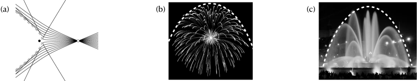
The positive energy analog of Proposition 4.13, i.e. for hyperbolic orbits, is somewhat disappointing, as the family admits no envelope. There is however a ‘scattering’ version of this proposition, for the repelling inverse square law, see Figure 14(i). A familiar ‘everyday’ version, for constant force, where all orbits as well as the envelope are parabolas, can be observed in fireworks displays and water fountains. See Figure 14(b) and (c).

5 Proofs of Theorems 1-6

Proof of Theorem 1.

Let $\mathbb{R}P^{3}$ be the 3-dimensional projective space with homogeneous coordinates $(X:Y:Z:W)$ . We identify $\mathbb{R}^{3}$ with the affine chart $W\neq 0$ , $(x,y,z)\mapsto(x:y:z:1).$ The closure of $\mathcal{C}=\{x^{2}+y^{2}=z^{2}\}$ in $\mathbb{R}P^{3}$ is $\overline{\mathcal{C}}=\{X^{2}+Y^{2}=Z^{2}\}$ , obtained by adding to $\mathcal{C}$ the ‘circle at infinity’ $S^{1}_{\infty}=\{X^{2}+Y^{2}=Z^{2},\ W=0\}=\overline{\mathcal{C}}\setminus\mathcal{C}$ . See Figure 3.

Let $\widetilde{\mathcal{G}}\subset\mathrm{GL}_{4}(\mathbb{R})$ be the subgroup preserving the (degenerate) quadratic form $X^{2}+Y^{2}-Z^{2}$ , up to scale. Its image $\mathcal{G}:=\widetilde{\mathcal{G}}/\mathbb{R}^{*}$ in the projective group $\mathrm{PGL}_{4}(\mathbb{R})=\mathrm{GL}_{4}(\mathbb{R})/\mathbb{R}^{*}$ is the group of projective transformations of $\mathbb{R}P^{3}$ preserving $\overline{\mathcal{C}}$ .

Lemma 5.1.

$\widetilde{\mathcal{G}}$ consists of elements of the form

\left(\begin{array}[]{cc}A&0\\ {\bf b}^{t}&\lambda\\ \end{array}\right),\quad A\in\mathrm{CO}_{2,1},\ {\bf b}\in\mathbb{R}^{3},\ \lambda\in\mathbb{R}\setminus 0.

(10)

Proof.

$g\in\widetilde{\mathcal{G}}$ if and only if $g^{t}Jg=cJ$ , where $J=\mathrm{diag}(1,1,-1,0)$ and $c\in\mathbb{R}$ . By a simple calculation $g$ has the claimed form. $\square$

It follows that $\widetilde{\mathcal{G}}$ is an 8-dimensional group and $\mathcal{G}=\widetilde{\mathcal{G}}/\mathbb{R}^{*}$ is 7-dimensional. In the affine chart $\mathbb{R}^{3}\subset\mathbb{R}P^{3}$ (column vectors), ${\mathbf{q}}\mapsto({\mathbf{q}}:1)$ , the action of an element of $\widetilde{\mathcal{G}}$ given by Equation (10) is

{\mathbf{q}}\mapsto\frac{A{\mathbf{q}}}{\lambda+{\bf b}^{t}{\mathbf{q}}},\quad{\mathbf{q}}\in\mathbb{R}^{3}.

(11)

It restricts to a local action on $\mathcal{C}_{+}$ and projects to a local action on $\mathbb{R}^{2}\setminus 0$ . By the general theory of point symmetries of ODEs (see the Appendix), the maximal dimension of the symmetry group of a 3-parameter family of plane curves is 7, hence this local $\mathcal{G}$ -action on $\mathbb{R}^{2}\setminus 0$ provides the full group of orbital symmetries.

The expressions for the infinitesimal symmetries in Equation (1) follow from the above by differentiating the action along 1-parameter subgroups of $\widetilde{\mathcal{G}}$ . Let $X\in\mathrm{Lie}(\widetilde{\mathcal{G}})$ (the Lie algebra of $\widetilde{\mathcal{G}}$ ). Since we are considering projectivized action, we can assume without loss of generality that ${\rm tr}(X)=0$ . From Equation (10) follows that such an $X$ has the form

X=\left(\begin{array}[]{cccc}\frac{x_{1}}{4}&-x_{2}&x_{3}&0\\ x_{2}&\frac{x_{1}}{4}&x_{4}&0\\ x_{3}&x_{4}&\frac{x_{1}}{4}&0\\ x_{5}&x_{6}&x_{7}&-\frac{3x_{1}}{4}\\ \end{array}\right),\ x_{1},\ldots,x_{7}\in\mathbb{R}.

(12)

The induced vector field on $\mathbb{R}^{2}\setminus 0$ is $(x,y)\mapsto\gamma^{\prime}(0),$ where $\gamma(t)=\pi(e^{tX}q)$ , $q=(x,y,\sqrt{x^{2}+y^{2}},1)^{t}$ and $\pi(X,Y,Z,W)=\left(X/W,Y/W\right).$ The formulas of Equation (1) follow from this recipe by setting $x_{i}=1$ and the rest 0 in Equation (12), $i=1,\ldots,7.$ $\square$

Proof of Theorem 2.

Note first that an element $g\in\widetilde{\mathcal{G}}$ , given by Equation (10), acts on $(\mathbb{R}^{4})^{*}$ (row vectors) by $p\mapsto pg^{-1}$ . In the affine chart $\mathbb{R}^{2,1}\subset\mathrm{P}((\mathbb{R}^{4})^{*})$ (row vectors), ${\mathbf{p}}\mapsto({\mathbf{p}}:-1)$ , the action on $\mathbb{R}^{2,1}$ by an element of $\widetilde{\mathcal{G}}$ , given by Equation (10), is

{\mathbf{p}}\mapsto(\lambda{\mathbf{p}}+{\bf b}^{t})A^{-1},\ {\mathbf{p}}\in\mathbb{R}^{2,1}.

(13)

It follows that for $X$ given by Equation (12) the induced vector field on $\mathbb{R}^{2,1}$ is ${\mathbf{p}}\mapsto\gamma^{\prime}(0),$ where $\gamma(t)=\pi(pe^{-tX})$ , $p=({\mathbf{p}},-1)$ and $\pi(A,B,C,D)=-\left(A/D,B/D,C/D\right).$ $\square$

Proof of Theorem 3.

Identify $\mathbb{R}^{2}=\mathbb{C}$ and consider the squaring map $B:{\mathbf{z}}\mapsto{\mathbf{z}}^{2}.$

Lemma 5.2.

$B$ defines a $2:1$ cover $\mathbb{C}\setminus 0\to\mathbb{C}\setminus 0$ , mapping pairs of parallel symmetric affine lines into Kepler parabolas.

Proof.

Since $B$ is $\mathbb{C}^{*}$ -equivariant, $B(\lambda Z)=\lambda^{2}B(Z),$ $\lambda\in\mathbb{C}^{*}$ , it is enough to consider the pair $x=\pm 1$ . Their $B$ -image is the Kepler parabola $x=(1+y/2)^{2}.$ $\square$

It follows that the set of Kepler parabolas is a flat 2-parameter family of plane curves. $\square$

Proof of Theorem 4.

We offer two proofs.

First proof. Kepler orbits with angular momentum $M$ are the projections of sections of $\mathcal{C}$ by planes passing through $P:=(0,0,M^{2})$ (Corollary 3.4). Central projection from $P$ then maps these conic sections to straight lines in the $xy$ plane.

Second proof. Kepler orbits with fixed $M$ are parametrized by the horizontal plane $\{c=1/M^{2}\}\subset\mathbb{R}^{2,1}$ , see Corollary 3.4 above. We know that $\mathcal{G}$ acts on $\mathbb{R}^{2,1}$ as its full group of Minkowski similarities, so there is an element $g\in\widetilde{\mathcal{G}}$ that translates this plane to the plane $c=0$ , parametrizing straight lines in the $xy$ plane. By Equation (13), we can take $g$ corresponding to $A=id,{\bf b}=(0,0,-1/M^{2})$ . The stated formula follows from Equation (11). $\square$

Remark 5.3.

Yet another proof, less elementary, is to write a second order linear ODE for the family of Kepler orbits with fixed $M$ and use the fact that second order linear ODEs are flat [7, page 44]. The said ODE is $\rho^{\prime\prime}(\theta)+\rho(\theta)=1/M^{2},$ where $\rho=1/r$ . See the proof of Proposition A.2 below.

Proof of Theorem 5.

According to the general theory of symmetries of ODEs, flatness of a 2-parameter family of plane curves is equivalent to the vanishing of certain two differential invariants of an associated second order ODE. In the Appendix we carry out a calculation showing that one of these invariants is non-vanishing for the family of Kepler orbits of fixed non-zero energy, thus proving that each such family is non-flat, see Proposition A.2. Next, according to another basic result of the theory, the dimension of the symmetry group of a non-flat 2-parameter family is at most 3. Thus, for each $E\neq 0$ , it is enough to find a 3-dimensional subgroup of $\mathcal{G}$ preserving the set of Kepler orbits with energy $E$ .

As explained in Corollary 3.5, Kepler orbits with energy $\pm E\neq 0$ are projections of sections of $\mathcal{C}$ by planes tangent to the inscribed paraboloid of revolution $\mathcal{P}=\{2z=|E|\left(x^{2}+y^{2}\right)+1/|E|\}$ . Let $\overline{\mathcal{P}}$ be the closure of $\mathcal{P}$ in $\mathbb{R}P^{3}$ . It is a smooth convex compact surface, given in homogeneous coordinates by the vanishing of the quadratic form $|E|\left(X^{2}+Y^{2}\right)-2ZW+W^{2}/|E|,$ obtained by adding to $\mathcal{P}$ the point $(0:0:1:0)$ , the tangency point of $\overline{\mathcal{P}}$ with the plane $W=0$ (the white dot in Figure 15(a)). Consider the subgroup $\widetilde{\mathcal{G}}_{E}\subset\widetilde{\mathcal{G}}$ preserving this quadratic form up to scale. A short calculation shows that its Lie algebra consists of matrices of the form

X=\left(\begin{array}[]{cccc}0&-x_{2}&x_{3}&0\\ x_{2}&0&x_{4}&0\\ x_{3}&x_{4}&0&0\\ |E|x_{3}&|E|x_{4}&0&0\\ \end{array}\right),\quad x_{2},x_{3},x_{4}\in\mathbb{R}.

(14)

The associated vector field in the $xy$ -plane is $(x,y)\mapsto\gamma^{\prime}(0)$ , where $\gamma(t)=\pi(e^{tX}q)$ , $q=(x,y,\pm\sqrt{x^{2}+y^{2}},1)^{t}$ and $\pi(X,Y,Z,W)=\left(X/W,Y/W\right).$ The sign in $q$ is the opposite sign of $E$ , since for $E>0$ (the hyperbolic case) we need to project the action from $\mathcal{C}_{-}$ and for $E<0$ from $\mathcal{C}_{+}$ . Setting $x_{i}=1$ and the rest 0 in Equation (14), $i=2,3,4,$ we obtain from this recipe for $E<0$ the vector fields

v_{2}:=\partial_{\theta},\ v_{3}:=r(\partial_{x}+Ex\partial_{r}),\ v_{4}:=r(\partial_{y}+Ey\partial_{r}),

as in Equation (3). For $E>0$ we get the vector fields $v_{2},-v_{3},-v_{4}.$ In both cases, $v_{2},v_{3},v_{4}$ are infinitesimal generators of the $\mathcal{G}_{E}$ -action, as stated.

The isomorphism $\widetilde{\mathcal{G}}_{E}/\mathbb{R}^{*}\simeq\mathrm{PSL}_{2}(\mathbb{R})$ is best seen in the dual picture, in $\mathbb{R}^{2,1}$ . See Figure 15(b).

Kepler orbits of energy $E\neq 0$ are parametrized by the surface $\mathcal{P}^{*}=\{-a^{2}-b^{2}+(c-|E|)^{2}=E^{2}\}\subset\mathbb{R}^{2,1}$ , the quadric surface dual to $\overline{\mathcal{P}}$ (see Equation (7) and Figure 15(b)). This is a hyperboloid of revolution of two sheets. The lower sheet $\mathcal{P}^{*}_{+}$ parametrizes planes tangent to $\mathcal{P}_{+}$ , which correspond to Kepler hyperbolas with energy $|E|$ . Similarly for the lower sheet. The Lorentzian metric $da^{2}+db^{2}-dc^{2}$ in $\mathbb{R}^{2,1}$ restricts to an hyperbolic metric on each of the sheets, on each of which the identity component of $\mathcal{G}_{E}$ acts as the identity component of its isometry group (in the full $\mathcal{G}_{E}$ there is also an element interchanging the two sheets, we will use it in the proof of the next theorem).

It is also clear from Figure 15(a) why the orbital symmetry action on $\mathcal{H}_{E}$ for $E>0$ is only local. This is because $\overline{\mathcal{P}}_{+}$ touches the plane $W=0$ (the ‘plane at infinity’ of the affine chart $W=0$ , intersecting $\overline{\mathcal{C}}$ at $S^{1}_{\infty}$ ) at one point, which does not correspond to any point in Kepler’s $xy$ plane. $\square$

Proof of Theorem 6.

Consider in Figure 15(b) the reflection about the horizontal plane $c=|E|$ passing through the vertex of the shown cone, $(a,b,c)\mapsto(a,b,2|E|-c),$ interchanging the lower and upper sheets $\mathcal{P}^{*}_{\pm}$ of $\mathcal{P}^{*}$ . The corresponding element in $\widetilde{\mathcal{G}}$ is

g=\left(\begin{array}[]{cccc}1&0&0&0\\ 0&1&0&0\\ 0&0&-1&0\\ 0&0&-2|E|&1\\ \end{array}\right).

In Figure 15(a), in the affine chart $Z\neq 0$ with coordinates $x=X/Z,y=Y/Z,w=W/Z$ , $g$ acts by $(x,y,w)\mapsto(x,y,2|E|-w)$ , a reflection about the center $(0,0,|E|)$ of $\overline{\mathcal{P}}$ (the dark dot), interchanging $\overline{\mathcal{P}}_{\pm}$ . In Figure 5, in the affine chart $W\neq 0$ , with coordinates $x=X/W,y=Y/W,z=Z/W$ , $g$ acts by $(x,y,z)\mapsto(x,y,-z)/(1-2|E|z),$ interchanging $\mathcal{P}_{\pm}.$

To write an explicit orbital embedding $\mathcal{H}_{E}\to\mathcal{H}_{-E}$ , note first in Figure 5 that Kepler hyperbolas are the projections of sections of the lower part $\mathcal{C}_{-}$ with planes tangent to $\mathcal{P}_{+}$ , and that Kepler ellipses are the projections of sections of the upper part $\mathcal{C}_{+}$ with planes tangent to $\mathcal{P}_{-}$ . The embedding is thus given by the composition ${\mathbf{r}}=(x,y)\mapsto({\mathbf{r}},-r)\mapsto({\mathbf{r}},r)/(1+2Er)\mapsto{\mathbf{r}}/(1+2Er),$ as needed.

We can also map the ‘repelling branches’ of Kepler hyperbolas with energy $E$ into $\mathcal{H}_{-E}$ , but these are the projections of sections of the upper part of $\mathcal{C}$ with planes tangent to $\mathcal{P}_{+}$ , thus the embedding is ${\mathbf{r}}=(x,y)\mapsto({\mathbf{r}},r)\mapsto({\mathbf{r}},-r)/(1-2Er)\mapsto{\mathbf{r}}/(1-2Er).$ See Figure 6. $\square$

Appendix A Appendix: Symmetries of ODEs

The purpose of this appendix is twofold: first, we fulfill a promise made in the beginning of the proof of Theorem 5, showing that the 2-parameter family of Kepler orbits with fixed non-zero energy is not flat. See Theorem 10 below. Second, we fit the results of this article into the general context of the theory of symmetries of ODEs.

Lie’s theory of symmetries of ODEs.

An $n$ -parameter family of plane curves is given, locally, under some mild regularity conditions, by the graphs of solutions $y(x)$ of an $n$ -th order ODE $y^{(n)}=f(x,y,y^{\prime},\ldots,y^{(n-1)}).$ Local diffeomorphisms of the $xy$ plane preserving the graphs of solutions of the ODE are classically called point symmetries of the ODE. Vector fields in the plane whose flow acts by point symmetries are infinitesimal point symmetries. The subject was developed in the 19th century, mostly by Sophus Lie and his students, later on in the 20th century by É. Cartan and many others, and is a still an active area of research. A standard modern reference is P. Olver’s book, see also [13, 20, 38, 43].

On ‘local symmetries’.

Point symmetries are local not only in the $xy$ plane but also in the jet spaces over $\mathbb{R}^{2}$ to which they are naturally prolonged. An $n$ -th order ODE $y^{(n)}=f(x,y,y^{\prime},\ldots,y^{(n-1)})$ defines a hypersurface $M:=\{p_{n}=f(x,y,p_{1},\ldots,p_{n-1})\}$ in the total space $J^{n}$ of the bundle of $n$ -th order jets of curves in $\mathbb{R}^{2}$ . $M$ is an $(n+1)$ -dimensional manifold, doubly foliated, with leaves of dimensions $n-1$ , $1$ , the sum of whose tangents span a contact distribution on $M$ . The first foliation is by the fibers of the projection $(x,y,p_{1},\ldots,p_{n})\mapsto(x,y)$ and the second by the $n$ -th jets of the solutions to the ODE. A point symmetry of the ODE is a local diffeomorphism of $M$ preserving both foliations. It projects to a local diffeomorphism of the $xy$ plane. A good introduction to this geometric point of view on ODEs, for $n=2$ , is Arnold’s book [7, Section 1.6].

Flat families.

An $n$ -parameter family of plane curves is flat if it is locally diffeomorphic to the family given by $y^{(n)}=0$ (graphs of polynomial functions of degree $<n$ ). As was shown by S. Lie, a family is flat if and only if its local symmetry group is $(n+4)$ -dimensional for $n>2$ and 8-dimensional for $n=2$ , the maximal dimension possible for an $n$ -parameter family of plane curves (Theorems 6.39 and 6.42 of [37]).

The $n=3$ case, i.e. point symmetries of 3rd order ODEs, was further studied in more depth in 1905 by K. Wünschmann [46], around 1940 by S.-s Chern [17, 18] and É. Cartan [16], and later on by others [24, 25, 26, 40, 45]. The only result from this theory that we use, in the proof of Theorem 1, due to Lie, is that the maximum dimension of the symmetry group of a 3-parameter family of plane curves is 7.

Theorem 1 can thus be interpreted as saying that the 3-parameter family of Kepler orbits is locally diffeomorphic to the solutions of $y^{\prime\prime\prime}=0,$ i.e. vertical parabolas of the form $y=ax^{2}+bx+c.$ Let us find such a diffeomorphism. Define a map from the $XY$ plane to the $xy$ -plane by

(X,Y)\mapsto(x,y)=\left({X^{2}-1\over Y},{2X\over Y}\right).

(15)

Proposition A.1.

Equation (15) defines a local diffeomorphism from the $XY$ -plane into the $xy$ -plane, mapping each vertical parabola $Y=AX^{2}+BX+C,$ $A,B,C\in\mathbb{R}$ , onto the Kepler orbit $ax+by+cr=1$ , where $a=(A-C)/2,b=B/2,c=(A+C)/2.$

The proof is by a straightforward verification.

Path geometries, Tresse classification.

The $n=2$ case is the best known and is called a path geometry. If a 2-parameter family is not flat then the maximal possible dimension of the symmetry group drops from 8 to 3. A list of normal forms of 2nd order ODEs admitting a 3-dimensional group of symmetries, over the complex numbers, was derived by A. Tresse (a French student of S. Lie) in his 1896 PhD dissertation [44]. The list is divided into 4 ‘types’, according to the symmetry group (all types come with 1 or 2 continuous parameters). Type d), the type that concerns us, deals with $\mathrm{SL}_{2}(\mathbb{C})$ invariant 2nd order ODEs, and is given by Tresse as $y^{\prime\prime}=(a(y^{\prime})^{3}-y^{\prime})/(6x),$ where $a$ is a (complex) parameter.

Tresse classification was extended to the real case [21, 31] but by and large we think that this list has not been sufficiently explored.

Over the reals, Tresse’s type d) breaks first into two subtypes, according to the two real forms of $\mathrm{SL}_{2}(\mathbb{C})$ : $\mathrm{SU}_{2}$ and $\mathrm{SL}_{2}(\mathbb{R})$ . We are concerned with $\mathrm{SL}_{2}(\mathbb{R})$ .

Among the ${\mathrm{SL}_{2}(\mathbb{R})}$ -invariant path geometries, there are two ‘exceptional’ cases (without parameters), corresponding to the two ODEs $y^{\prime\prime}=\pm(xy^{\prime}-y)^{3}$ . What distinguishes these two cases from all other items on Tresse list is that these are the only cases of projective path geometries, i.e. the paths are the (unparametrized) geodesics of a torsionless affine connection. In fact, in this case the paths are the geodesics of the well known Jacobi-Maupertuis metric defined on the Hill region for any mechanical system with fixed energy.

The case that appears here (constant energy Kepler orbits) corresponds to $y^{\prime\prime}=(xy^{\prime}-y)^{3}$ , but it is not so easy to see the equivalence (we will not pursue it here).

A path geometry on a surface $S$ determines a ‘dual’ path geometry on the path space $S^{*}$ , parametrized by the points of $S$ : to each point of $S$ is assigned a path in $S^{*}$ , the set of paths in $S$ passing through this point. The dual path geometry of a flat path geometry (straight lines, graphs of solutions to $y^{\prime\prime}=0$ ) is also flat, but a generic non-flat path geometry is not equivalent to its dual. The flatness of a path geometry, given by a 2nd order ODE $y^{\prime\prime}=f(x,y^{\prime},y^{\prime\prime})$ , is detected by the vanishing of the relative invariants

\displaystyle\begin{split}I_{1}=&f_{pppp},\\ I_{2}=&D^{2}f_{pp}-4Df_{py}+f_{p}(4f_{py}-Df_{pp})-3f_{pp}f_{y}+6f_{yy},\end{split}

(16)

where $p=y^{\prime}$ and $D=\partial_{x}+p\partial_{y}+f\partial_{p}.$

The vanishing of $I_{1}$ simply means that $F$ is at most cubic in $y^{\prime}$ . This is a diffeomorphism invariant property, characterizing projective path geometries. The vanishing of $I_{2}$ is equivalent to the projectivity of the dual path geometry. Thus a path geometry is flat if and only if it is projective and its dual path geometry is projective as well.

Kepler orbits of fixed energy.

We can now fill the gap left out in the proof of Theorem 5.

Proposition A.2.

Kepler orbits of fixed energy $E\neq 0$ form a non-flat path geometry. In fact, $I_{1}=0$ but $I_{2}\neq 0$ . Thus the maximum dimension of the symmetry group of such a family is 3.

Proof.

We 1st write down a 2nd order ODE for Kepler orbits of energy $E$ . Using the equation $ax+by+cr=1$ of Theorem 7(a), we get

\rho=a\cos\theta+b\sin\theta+c,\ \rho^{\prime}=-a\sin\theta+b\cos\theta,\ \rho^{\prime\prime}=-a\cos\theta-b\sin\theta,

where $x=r\cos\theta,y=r\sin\theta,r=1/\rho.$ It follows that

\rho+\rho^{\prime\prime}=c,\ (\rho^{\prime})^{2}+(\rho^{\prime\prime})^{2}=a^{2}+b^{2}.

Using this in $2cE=a^{2}+b^{2}-c^{2}$ (Equation (7) with $c>0$ ), we get,

\rho^{\prime\prime}={\rho^{2}+\rho^{\prime 2}\over 2(\rho+E)}-\rho.

Using Equations (16) we get $I_{2}=9E^{2}/(E+\rho)^{3},$ hence $I_{2}\neq 0$ for $E\neq 0.$ $\square$

Remark A.3.

Incidentally, the formula $I_{2}=9E^{2}/(E+\rho)^{3}$ of the last proof gives another proof of Theorem 3.

Central forces with flat orbit space. The Wünschman condition.

Theorem 1 establishes that Kepler orbits form a flat 3-parameter family of curves, i.e. locally diffeomorphic to the family of vertical parabolas, given by $y^{\prime\prime\prime}=0$ . Using the squaring map, ${\mathbf{z}}\mapsto{\mathbf{z}}^{2}$ , this result extends to Hooke orbits, the family of central conics, trajectories of a mass under Hooke’s force laws, $\ddot{\mathbf{r}}=\pm{\mathbf{r}}.$ Are there any other force laws, whose orbits form a flat family of plane curves?

We do not know the answer in general. But for central force laws, i.e. Newton’s equations of the form $\ddot{\mathbf{r}}=f(r){\mathbf{r}}/r,$ the answer is negative. To prove it, we show that in fact the Hooke and Kepler laws are the only central force laws satisfying a condition weaker than flatness, called the Wünschman condition (1905). Given a 3-parameter family of plane curves, one defines null cones in the parameter space whose rulings consist of the curves that are tangent to a fixed line at a fixed point. In the flat case, such as the space of Kepler orbits, these cones are quadratic and thus define a (flat) conformal structure on the parameter space. However, for a general family, these cones may fail to be quadratic. The families for which the null cones are quadratic, and hence define a conformal Lorentzian metric on the parameter space, are characterized by a complicated PDE on the ODE that defines this family, studied by K. Wünschmann [46]. For a modern presentation of this deep result see [36].

Theorem 10.

The orbits of the system $\ddot{\mathbf{r}}=f(r){\mathbf{r}}/r$ form a flat 3-parameter family of plane curves if and only if $f(r)$ is a constant multiple of $r$ or $1/r^{2}$ . In fact, these force laws are the only central ones satisfying the Wünschmann condition.

Proof.

Following the standard procedure outlined above, we first write a 3rd order ODE whose solutions are the (unparametrized) orbits of the system $\ddot{\mathbf{r}}=f(r){\mathbf{r}}/r$ ,

\rho^{\prime\prime\prime}=\rho^{\prime}\left[(\rho^{\prime\prime}+\rho)\left({f^{\prime}(\rho)\over f(\rho)}-{2\over\rho}\right)-1\right],

(17)

where $\rho=1/r,$ $\rho=\rho(\theta)$ (see for example [29]). Next, the Wünschmann condition for $\rho^{\prime\prime\prime}=F(\rho,\rho^{\prime},\rho^{\prime\prime})$ is

F_{\rho}+\left(D-{2\over 3}F_{\rho^{\prime\prime}}\right)K=0,

where

K={1\over 6}DF_{\rho^{\prime\prime}}-{1\over 9}F_{\rho^{\prime\prime}}^{2}-{1\over 2}F_{\rho^{\prime}},\quad D=\partial_{\theta}+\rho^{\prime}\partial_{\rho}+\rho^{\prime\prime}\partial_{\rho^{\prime}}+F^{\prime}\partial_{\rho^{\prime\prime}}.

See [36, Equation 8]. Applying this condition to the right hand side of Equation (17), we get a pair of ODEs for $f(\rho)$ , whose only solutions are constant multiples of $\rho^{2}$ and $1/\rho.$ $\square$

Central forces and projective path geometries.

As mentioned above, in the local classification of path geometries admitting a 3-dimensional group of symmetries there are only 3 projective cases, where the paths arise as the unparametrized geodesics of a torsionless affine connection. In general, a projective path geometry need not be a metric path geometry, i.e. the affine connection may not be the Levi-Civita connection of a pseudo-Riemannian metric, but in our 3 cases they are metric connections. In fact, all 3 cases arise as the orbits of fixed energy of conservative mechanical systems, and thus can be realized as geodesics of the associated Jacobi-Maupertuis metric. Let us list the 3 cases by 2nd order ODEs defining them:

I.

$y^{\prime\prime}=0$ .
II.

$y^{\prime\prime}=(xy^{\prime}-y)^{3}$
III.

$y^{\prime\prime}=-(xy^{\prime}-y)^{3}$

(See e.g. [21], where our type I is item 4 of Theorem 7 and our types II and III are items $3d_{+}$ and $3d_{-}$ , respectively.)

Type I is the flat path geometry, admitting an $8$ -dimensional symmetry group, the projective group $\mathrm{PGL}_{3}(\mathbb{R})$ . Type II and III are non-flat, each admitting ${\mathrm{SL}_{2}(\mathbb{R})}$ as a local symmetry group. In both types II and III the ${\mathrm{SL}_{2}(\mathbb{R})}$ action is locally equivalent to the standard linear action on $\mathbb{R}^{2}\setminus 0$ . The dual actions, on the dual path geometries, are non equivalent: for the dual of type II ${\mathrm{SL}_{2}(\mathbb{R})}$ acts by isometries of the hyperbolic plane and in the dual of type III as isometries of pseudo-hyperbolic plane (non-flat constant curvature Lorentzian metric). Both actions appear naturally as open orbits of the projectivized adjoint representation of ${\mathrm{SL}_{2}(\mathbb{R})}$ .

In Table 2 we place some 2-parameter families of curves arising naturally in planar mechanical systems with central-force laws, locally realizing the 3 path geometries. In the 1st two rows we consider central-force power laws, $\ddot{\mathbf{r}}=f(r){\mathbf{r}}/r,$ $f(r)=\pm r^{\alpha},$ where $M$ and $E$ are the (fixed) angular momentum and energy, respectively. In parentheses is the force law ( $\pm r^{\alpha}$ , with ‘–’ for attractive and ‘+’ for repelling). In the following two rows $E_{k}$ is the energy, $M_{k}$ the angular momentum, for the Kepler problem in a space of constant curvature $k$ , as in [2].

Table 2: Projective path geometries and central-force laws

I. $y^{\prime\prime}=0$ .	II. $y^{\prime\prime}=(xy^{\prime}-y)^{3}$	III. $y^{\prime\prime}=-(xy^{\prime}-y)^{3}$
$M\neq 0$ , ( $\pm 1/r^{2},\pm 1/r^{3}$ )	$M\neq 0$ , ( $-r$ )	$M\neq 0$ , ( $r$ )
$E=0$ , ( $\pm r^{\alpha}$ , $\alpha\neq-1$ )	$E\neq 0$ , ( $\pm 1/r^{2},\pm r$ )	–
$\|E_{k}\|=\sqrt{-k}$ , $k<0$	$\|E_{k}\|>\sqrt{-k}$ , $k<0$	$\|E_{k}\|<\sqrt{-k}$ , $k<0$
$M_{k}\neq 0$	$E_{k}$ , $k>0$	–

Some comments on Table 2.

1. ‘Hooke’ orbits, attractive or repelling ( $f=\pm r$ ), with fixed angular momentum $M$ , were placed in the table by considering the squaring map, ${\mathbf{z}}\mapsto{\mathbf{z}}^{2}$ . They are thus mapped to Kepler orbits with fixed minor axis. Attractive Hooke orbits ( $f=-r$ ) are mapped to Kepler ellipses with fixed minor axis (see item 1 of Table 1 and Lemma 4.15), which are equivalent to ellipses of constant energy (see proof of Corollary 4.6), corresponding to type II path geometry. Repelling Hooke orbits ( $f=r$ ) are mapped to Kepler hyperbolas with fixed minor axis (item 1 of Table 1), which is type III path geometry.

2. Zero energy orbits for all central-force power laws, $f=\pm r^{\alpha}$ , $\alpha\neq-1$ , can be seen to give a flat path geometry (type I) by using the Jacobi-Maupertuis metric: by making the change of variable $r=\rho^{2/(\alpha+3)}$ for $\alpha\neq-3$ , or $r=e^{\rho}$ for $\alpha=-3$ , one shows that such families are equivalent to geodesics on a quadratic cone, so are locally equivalent to lines in the plane [34, §4]. More generally, for planar motion $\ddot{\mathbf{r}}=-\nabla U$ , with potential satisfying $\Delta\log U=\lambda U$ for some $\lambda\in\mathbb{R}$ , the orbits at energy zero will also be locally flat.

3. By computing the relative invariants $I_{1},I_{2}$ of Equation (16), it can be shown that orbits with fixed non-zero energy are non-flat for all central-force power laws. It also shows that zero energy orbits for $f=\pm r^{\alpha}$ are flat if and only if $\alpha\neq-1$ . Furthermore, by using additional (relative) invariants [21, §6], one finds that these path geometries admit a 3-dimensional symmetry group only for the Hooke and Kepler laws ( $\alpha=1,-2$ ).

4. Using $I_{1},I_{2}$ , it can be also shown that among all central-force power laws, orbits at a fixed non-zero angular momentum are flat only for the Kepler and inverse cubic force laws ( $\alpha=-2,-3$ ).

References

[1] A. Albouy, Projective dynamics and classical gravitation, Regul. Chaot. Dyn. 13 (2008), 525-542 .
[2] A. Albouy, There is a Projective Dynamics, Eur. Math. Soc. Newsl. 89 (2013), 37-43.
[3] A. Albouy, Lectures on the two-body problem. In: Classical and celestial mechanics: the Recife lectures, eds. H. Cabral, F. Diacu. Princeton University Press, 2002.
[4] A. Albouy, Lambert’s theorem: geometry or dynamics?, Celestial Mechanics and Dynamical Astronomy 131.9 (2019), 1-30.
[5] V. I. Arnold, Huygens and Barrow, Newton and Hooke: Pioneers in mathematical analysis and catastrophe theory from evolvents to quasicrystals. Birkhäuser, Basel (1990).
[6] V. I. Arnold, Mathematical methods of classical mechanics. Springer, 2nd Ed (1989).
[7] V. I. Arnold, Geometrical methods in the theory of ordinary differential equations. Springer Science & Business Media, Vol. 250 (2012).
[8] V. I. Arnold, Vassiliev, Newton’s Principia read 300 years later, Notices of the AMS 36.9 (1989), 1148-1154.
[9] J. Bertrand J, Théorème relatif au mouvement d’un point attiré vers un centre fixe, C. R. Acad. Sci. 77 (1873), 849-853. Available online: https://gallica.bnf.fr/ark:/12148/bpt6k3034n/f849. English translation: https://arxiv.org/abs/0704.2396
[10] P. Blaschke, Pedal coordinates, dark Kepler, and other force problems, J. Math. Phys. 58 (2017), 063505
[11] K. Bohlin, Note sur le problème des deux corps et sur une intégration nouvelle dans le problème des trois corps, Bull. Astr. 28 (1911), 113-119.
[12] G. Bor, C. Jackman, S. Tabachnikov, Variations on the Tait-Kneser theorem, preprint (2021). https://arxiv.org/abs/2104.02170
[13] G. W. Bluman, S. Kumei, Symmetries and Differential Equations. Springer-Verlag, New York (1989).
[14] R. Bryant, G. Manno, V. Matveev, A solution of S. Lie Problem: Normal forms of 2-dim metrics admitting two projective vector fields, Math. Ann. 340.2 (2008), 437-463.
[15] J. F. Cariñena, C. López, M. A. del Olmo, M. Santander, Conformal geometry of the Kepler orbit space, Celestial Mechanics and Dynamical Astronomy, 52.4 (1991), 307-343.
[16] É. Cartan, La geometría de las ecuaciones diferenciales de tercer orden, Rev. Math. Hispano-Amer. 4 (1941), 1-31. Reprinted in : Œuvres complètes, Partie III, vol. 2, 1535-1565. Gauthier-Villars, 1952.
[17] S.-s. Chern, Sur la géométrie d’une équation différentielle du troisième ordre. C. R. Acad. Sci., Paris 204 (1937), 1227–1229.
[18] S.-s. Chern, The geometry of the differential equations $y^{\prime\prime\prime}=F(x,y,y^{\prime},y^{\prime\prime})$ , Sci. Rep. Nat. Tsing Hua Univ. 4 (1940), 97–111.
[19] D. DeTurck, H. Gluck, D. Pomerleano, D.S. Vick, The Four Vertex Theorem and Its Converse. Notices of the AMS 54.2 (2007), 192-207.
[20] S.V. Duzhin, V.V. Lychagin, Symmetries of distributions and quadrature of ordinary differential equations, Acta Applicandae Mathematica, 24.1 (1991), 29-57.
[21] B. Doubrov, B. Komrakov, The geometry of second-order ordinary differential equations, preprint (2016). https://arxiv.org/abs/1602.00913
[22] U. Frauenfelder, O. Van Koert, The restricted three-body problem and holomorphic curves. Springer International Publishing, 2018.
[23] A. Givental, Kepler’s Laws and Conic Sections, Arnold Math J. 2 (2016), 139-148.
[24] M. Godlinski, Geometry of Third-Order Ordinary Differential Equations and Its Applications in General Relativity. PhD thesis, Univ. of Warsaw (2008). https://arxiv.org/abs/0810.2234
[25] M. Godlinski, P. Nurowski, Third-order ODEs and four-dimensional split signature Einstein metrics, J. Geom. Phys. 56.3 (2006), 344-357.
[26] M. Godlinski, P. Nurowski, Geometry of third-order ODEs, preprint (2009). https://arxiv.org/abs/0902.4129
[27] E. Ghys, S. Tabachnikov, V. Timorin, Osculating curves: around the Tait- Kneser theorem, Math. Intelligencer 35.1 (2013), 61-66.
[28] V. Guillemin, S. Sternberg, Variations on a Theme by Kepler. Vol. 42. American Mathematical Soc., 2006.
[29] E. Kasner, The Trajectories of Dynamics, Trans. Am. Math. Soc 7.3 (1906), 401–424.
[30] J. L. Lagrange, Recherches sur la théorie des perturbations, Mémoires des Savant étrangers, tome X, 1785. Reproduced in: Oeuvres complètes, tome 6, 419-431. Gauthier-Villars, Paris, 1873.
https://gallica.bnf.fr/ark:/12148/bpt6k229225j/
[31] J. Lang, Three Projective Problems on Finsler Surfaces, PhD thesis, Friedrich Schiller Universität Jena (2020). https://www.db-thueringen.de/receive/dbt_mods_00040622
[32] C. Maclaurin, A treatise of fluxions, Vol. 2. Edinburgh: Ruddimans, 1742.
[33] J. Milnor, On the Geometry of the Kepler Problem, Amer. Math. Monthly 90.6 (1983), 353-365.
[34] R. Montgomery, Metric cones, N-body collisions, and Marchal’s lemma, preprint (2018), https://arxiv.org/abs/1804.03059
[35] J. Moser, Regularization of Kepler’s problem and the averaging method on a manifold, Comm. Pure Appl. Math. 23 (1970), 609–636.
[36] P. Nurowski, Differential equations and conformal structures, J. Geom. Phys. 55.1 (2005), 19-49.
[37] P.J. Olver, Equivalence, Invariants and Symmetry. Cambridge University Press, 1995.
[38] G. Prince, J. Sherring, Geometric aspects of reduction of order, Trans. AMS 334.1 (1992), 433-453.
[39] J.-M. Richard, Safe domain and elementary geometry. European journal of physics, 25.6 (2004), 835-844.
[40] H. Sato, A.Y. Yoshikawa, Third order ordinary differential equations and Legendre connection, J. Math. Soc. Japan 50.4 (1998), 993-1013.
[41] V. G. Sezebehely, Adventures in celestial mechanics, a first course in the theory of orbits. U. Texas Press, 1989.
[42] J.M. Souriau, Sur la variété de Kepler. Centre de Physique Théorique, 1973.
[43] H. Stephani, Differential Equations: Their Solution Using Symmetries. Cambridge University Press, 1989.
[44] A. Tresse, Détermination des invariants ponctuels de l’équation différentielle ordinaire du second ordre $y^{\prime\prime}=\omega(x,y,y^{\prime})$ . Vol. 32. S. Hirzel, 1896.
[45] K. P. Tod, Einstein-Weyl spaces and third-order differential equations, J. Math. Phys. 41.8 (2000), 5572-5581.
[46] K. Wünschmann, Über Berührungsbedingungen bei Integralkurven von Differentialgleichungen. Inauguraldissertation, Leipzig, Teubner, 1905, 6-13.