Revisiting Intermediate Layer Distillation
for Compressing Language Models: An Overfitting Perspective

Jongwoo Ko¹
KAIST AI &Seungjoon Park¹
KAIST AI &Minchan Jeong¹
KAIST AI \ANDSukjin Hong²
KT &Euijai Ahn²
KT &Du-Seong Chang²
KT &Se-Young Yun¹
KAIST AI \AND¹{jongwoo.ko, sjoon.park, mcjeong, yunseyoung}@kaist.ac.kr
²{sukjin.hong, euijai.ahn, dschang}@kt.com

Abstract

Knowledge distillation (KD) is a highly promising method for mitigating the computational problems of pre-trained language models (PLMs). Among various KD approaches, Intermediate Layer Distillation (ILD) has been a de facto standard KD method with its performance efficacy in the NLP field. In this paper, we find that existing ILD methods are prone to overfitting to training datasets, although these methods transfer more information than the original KD. Next, we present the simple observations to mitigate the overfitting of ILD: distilling only the last Transformer layer and conducting ILD on supplementary tasks. Based on our two findings, we propose a simple yet effective consistency-regularized ILD (CR-ILD), which prevents the student model from overfitting the training dataset. Substantial experiments on distilling BERT on the GLUE benchmark and several synthetic datasets demonstrate that our proposed ILD method outperforms other KD techniques. Our code is available at https://github.com/jongwooko/CR-ILD.

1 Introduction

Recent advances in NLP have shown that using PLMs such as BERT Devlin et al. (2019) and RoBERTa Liu et al. (2019) on downstream tasks is effective. Although these models achieve state-of-the-art performances in various domains, the promising results of PLMs require numerous computation and memory costs. Deploying such large models on resource-constrained devices such as mobile and wearable devices is impractical. It is thus crucial to train computationally efficient small-sized networks with similar performance to that of large models.

KD is promising model compression technique where knowledge is transferred from a large and high-performing model (teacher) to a smaller model (student). KD has been shown to be reliable in reducing the number of parameters and computations while achieving competitive results on downstream tasks. Recently, KD has attracted more attention in the NLP field, especially due to large PLMs. However, it is clear that the original KD Hinton et al. (2015) is not performing well in terms of maintaining the performance of compressed PLMs and that it needs to have additional auxiliary training objectives Sun et al. (2019); Jiao et al. (2020).

ILD methods Jiao et al. (2020); Wang et al. (2020), which encourage the student model to extract knowledge from the Transformer layers of the teacher network, have demonstrated efficacy in improving student model performance and have become a de facto standard in KD. Despite of success of ILD methods, many research have been proposed to design layer mapping functions Li et al. (2020); Wu et al. (2020) or new training objective Park et al. (2021) to transfer the teacher’s knowledge better. These ILD methods transfer more knowledge to the student model from the intermediate Transformer layers of the teacher model. However, we find that the use of ILD in fine-tuning may induce performance degradation in some cases. As shown in Figure 1, while existing ILD methods such as TinyBERT Jiao et al. (2020) and BERT-EMD Li et al. (2020) work well on standard GLUE benchmark Wang et al. (2019), we observe that these methods have performance degradation compared to original KD on ill-conditioned datasets such as those with few-samples and label noise. Because few-sample Zhang et al. (2021) or heterogeneous datasets Jin et al. (2021); Liu et al. (2022) can be easily found in real-world datasets, the existing ILD methods, which show performance reduction in Figure 1, are hard to use in real-world applications.

To mitigate such performance degradation, we identify the main problem as that intermediate Transformer knowledge can incur overfitting on the training dataset of the student model. We further discover that distilling only the last Transformer layer knowledge and using supplementary tasks can alleviate the overfitting. Through our observations, we finally propose a simple yet effective method, consistency-regularized ILD (CR-ILD) with several analyses. Our main contributions are:

•

We design and conduct comprehensive experiments to identify that overfitting is one of the main problems for performance degradation of ILD in fine-tuning. To the best of our knowledge, this is the first study to find that existing ILD methods have overfitting issues.
•

Based on our findings, we propose the consistency regularized ILD (CR-ILD) that a student self-regularized itself from risk of overfitting from ILD. We further provide empirical (and theoretical) analyses for our proposed method.
•

We experimentally demonstrate that our proposed method achieves state-of-the-art performance on both standard GLUE and ill-conditioned GLUE (few samples and label noise), despite its simplicity.

2 Related Works

Model Compression of LMs.

Transformer encodes contextual information for input tokens Vaswani et al. (2017). In recent years, from the success of Transformer, Transformer-based models such as GPT Radford et al. (2018), BERT Devlin et al. (2019), and T5 Raffel et al. (2020) have become a new state of the arts, driving out recurrent or convolutional networks on various language tasks. However, the promising results of these models are accompanied by numerous parameters, which necessitate a high computation and memory cost for inference. Existing compression techniques can be categorized as low-rank matrix factorization Mao et al. (2020), quantization Bai et al. (2021), and KD Sun et al. (2019).

Knowledge Distillation for LMs.

KD is one of the most well-known neural model compression techniques. The goal of KD is to enable the student model with fewer parameters to achieve similar performance to that of the teacher model with a large number of parameters. In the recent few years, a wide range of different methods have been developed that apply data augmentation Jiao et al. (2020); Liang et al. (2021), adversarial training Rashid et al. (2021), and loss terms re-weighting Jafari et al. (2021) to reduce the performance gap between the teacher and the student. In another line in the NLP field, ILD-based methods have exhibited higher effectiveness over original KD Hinton et al. (2015) methods for compression PLMs. Sun et al. (2019) proposed the BERT-PKD to transfer representations of the [CLS] token of the teacher model. Jiao et al. (2020) proposed TinyBERT, which performed Transformer distillation in both pre-training and fine-tuning. Wang et al. (2020) distilled the self-attention module of the last Transformer layer of the teacher. Li et al. (2020) leveraged earth mover’s distance (EMD) to determine the optimal layer mapping between the teacher and student networks. Park et al. (2021) presented new KD objectives that transfer contextual knowledge via two types of relationships.

3 Observations: Two Things Everyone Should Know to Mitigate Overfitting

In this section, we identify that overfitting is the main problem for performance degradation while conducting ILD in fine-tuning. This overfitting problem can occur even in the standard GLUE benchmark. Moreover, the ill-conditioned dataset, where overfitting problems can occur more easily, induces a larger performance reduction. Furthermore, we investigate that this overfitting problem is able to be reduced by (1) distilling the last Transformer layer and (2) conducting ILD on supplementary tasks. While our suggested findings already have worked well in various domains Wang et al. (2020); Phang et al. (2018), these previous works under-explored the effects of the techniques. However, this is the first work to use such techniques with empirical justification for mitigating overfitting problems.

Among the various ILD objectives, we focus on the two most commonly used distillation objectives: multi-head attention (MHA) and intermediate representations (IR). Formally, for the student’s layer $\ell^{S}\in[1,M]$ , the loss function of MHA and IR are as follows:

	$\displaystyle\mathcal{L}_{\text{MHA}}^{\ell^{S}}$	$\displaystyle=\frac{1}{A_{h}}\sum_{a=1}^{A_{h}}\text{KLD}(\mathbf{A}^{T}_{m(\ell^{S}),a}\|\|\mathbf{A}^{S}_{\ell^{S},a})$		(1)
	$\displaystyle\mathcal{L}_{\text{IR}}^{\ell^{S}}$	$\displaystyle=\text{MSE}(\mathbf{H}^{T}_{m(\ell^{S})},\mathbf{W}^{\text{H}}\mathbf{H}^{S}_{\ell}),$		(2)

where $m(\cdot)$ is layer mapping function that returns teacher layer $m(\ell^{S})\in[1,L]$ . Note that KLD and MSE are Kullback-Leibler divergence and mean squared error, respectively. We denote $\mathbf{A}$ and $\mathbf{H}$ as MHA and IR. $T$ and $S$ are superscripts for the teacher and student model, and $a$ and $A_{h}$ indicate the index and the total number of multi-attention heads, respectively. Note that $\mathbf{W}^{\text{H}}$ is a learnable weight matrix for matching the dimension between representations of the teacher and student. Consistent with previous studies Sun et al. (2020); Jiao et al. (2020), we observe that sequential training of ILD and original KD Hinton et al. (2015) shows better than joint training of ILD and original KD. We conduct an experimental study on sequential training of ILD and original KD from our preliminary experiments. All the detailed descriptions of the scope of our empirical study are in Appendix C.1.

3.1 Layer Mapping: Distill Only the Last Transformer Layer

One of the biggest challenges of ILD methods is establishing a proper layer mapping function that determines layers of the teacher and student models to transfer knowledge. In this section, we observe that transferring layer-to-layer information leads student models to overfit training samples and is the primary reason for the degradation of student performance. Based on our findings, we suggest that the last layer distillation Wang et al. (2020, 2021) is promising layer mapping method. Our empirical analyses can explain the suggested technique’s success in terms of mitigating overfitting.

Main Observations.

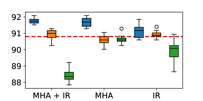
We compare three distillation strategies: last Transformer layer distillation (L-ILD), layer-to-layer distillation using uniform layer mapping (U-ILD), and optimal many-to-many layer mapping using the EMD (EMD-ILD) proposed in Li et al. (2020). In Figure 2, L-ILD (blue box) outperforms other baselines on all four datasets (MRPC, RTE, SST-2, QNLI) in terms of the test performance and variance reduction over the random trials. Note that the U-ILD, which is a commonly used mapping function Sun et al. (2019); Jiao et al. (2020), leads to performance degradation in most fine-tuning tasks.

We conduct same experiments on the student model with different initialization (BERT ${}_{\text{Small}}$ ; Turc et al. 2019) as shown in Figure 3. We observe that L-ILD has a higher performance regardless of the size of the dataset or initialized point. However, the performance gap between L-ILD and other mapping functions gets smaller when the dataset size becomes larger, and the student model is well pre-trained. On the other hand, although EMD-ILD alleviates the difficulties in layer mapping between the teacher and student, it exhibits lower performance than L-ILD. We find that performances of EMD-ILD vary across the pre-trained methods while performances of L-ILD are not. These results validate that the inaccurate layer mapping between the intermediate Transformer layers is not the primary problem of ILD; instead, intermediate Transformer layer distillation itself is the main problem in the fine-tuning stage.

Analysis.

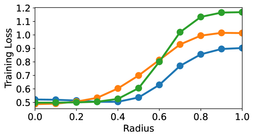
To better understand about the performance degradation of distilling the knowledge of intermediate Transformer layers, we evaluate the generalizability of the student models of different layer mapping functions by following Zhang et al. (2019); Jeong and Shin (2020). We add Gaussian noise over $\mathcal{N}(0,\sigma^{2}I)$ with different noise radius $\sigma$ to the embedding vectors of the three models (L-ILD, U-ILD, EMD-ILD) and then evaluate their cross-entropy loss on the training set. More generalizable models are robust to the noisy embeddings, hence they have a lower training loss although the magnitude of noise becomes larger.

As shown in Figure 4, transferring knowledge of the intermediate Transformer layers leads the student model to the flat minima that are robust of noise and more generalizable Hochreiter and Schmidhuber (1997); Keskar et al. (2016). We further conduct the loss surface Zhang et al. (2021) and linear probing Aghajanyan et al. (2021a) analyses for evaluating the generalizable representations of PLMs during fine-tuning and report the results in Appendix E.1.

3.2 Training Data: Use Supplementary Tasks

In this section, we investigate the performance of ILD in terms of training datasets for transferring knowledge from teacher to student model. We observe that conducting ILD even on the last Transformer layer has the risk of overfitting to the training dataset of target task (TT). The Previously suggested augmentation module in Jiao et al. (2020) generates 20 times the original data as augmented samples, requiring massive computational overhead for generating. From our observation, we find that conducting ILD via supplementary tasks (ST, Phang et al. 2018) is a simple and efficient method for overfitting problem. Based on our observation, we study to find the condition for appropriate ST, which robustly improves the performance of ILD.

Main Observations.

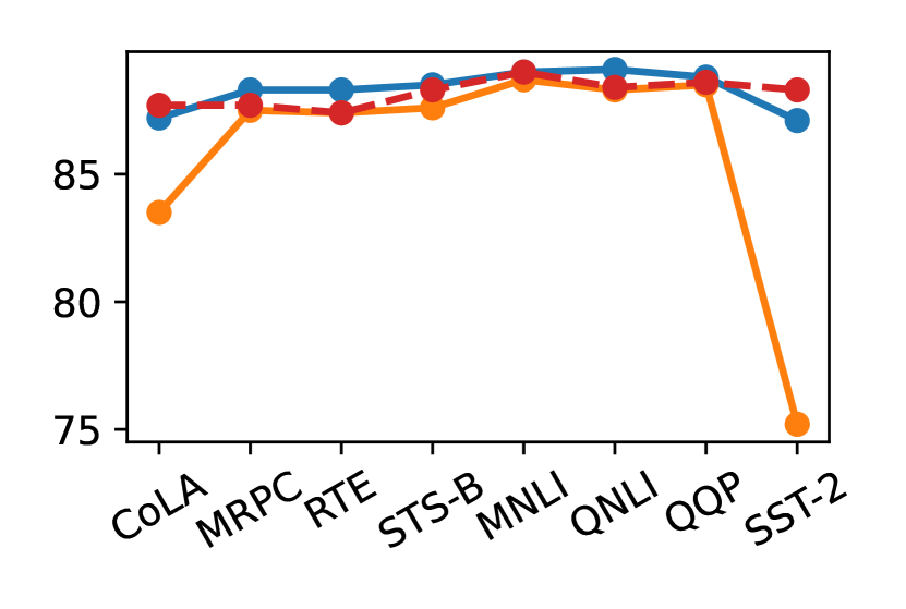
As shown in Figure 5, in most downstream tasks, except for STS-B, the performance of combining ILD with other STs is superior to that when using the original dataset. Among the tasks with small dataset (CoLA, MRPC, RTE, STS-B), although STS-B exhibits superiority as an ST for ILD, all student models with ILD on CoLA exhibit the worst performance for all TTs. For large tasks (MNLI, QNLI, QQP, SST-2) as STs, student models trained on MNLI and SST-2 exhibit the best and worst performance for all TTs.

Analysis.

To understand performance gain from using STs, we compare the loss dynamics for fine-tuning of RTE task using the cross-entropy loss after conducting ILD on the TT (RTE) and STs (MRPC, STS-B, QNLI). Notably, the student model with ILD on RTE shows a faster decrease and increase in the training and validation loss, respectively, than the student model with ILD on the STs, as shown in Figure 6. From the results, we verify that conducting ILD over TT incurs memorization of the student model to training data of TT while performing ILD over ST prevents this memorization yet effectively transfers knowledge of the teacher model.

3.2.1 Ablation Study

Although the combination of ST with ILD generally improves the performances of student models, decreased performances are observed in some cases. These results emphasize the need to select appropriate ST. In this section, we present exploratory experiments on synthetic datasets extracted from the English Wikipedia corpus to provide further intuition for the conditions of convincing STs.

Dataset Size.

According to the results in Figure 5, student models trained on STs with large datasets, such as MNLI and QQP, perform better. We conducted experiments on synthetic datasets extracted from the Wikipedia corpus with different dataset sizes to validate our observations. The results in Figure 7(a) and 7(b) indicate that as the size of the synthetic datasets grows larger, the performance of the student models improves.

Effective Sequence Length.

A surprising result of Figure 5 is that ILD on single sentence tasks such as SST-2 or CoLA exhibits lower performances than those of the smaller sentence pair tasks. This phenomenon is much more evident in U-ILD. Motivated by these results, we conducted experiments on synthetic datasets with the same dataset size of 30k and different effective sequence lengths (measured without considering [PAD] tokens). Figures 7(c) and 7(d) show that as the effective sequence length of the datasets increases, so do the performances of the student models.

Task Similarity.

Finally, we investigate the effect of task similarity between TTs and STs. We only use datasets in the GLUE benchmark for computing the similarity and do not use synthetic Wikipedia datasets. To measure the task similarity, we use the probing performance of the TT after performing ILD for each ST, following Pruksachatkun et al. (2020). We conduct ILD on different STs and then conduct probing and fine-tuning on the TT. Figure 7(e) and 7(f) summarize the correlation between the probing and fine-tuning performances for CoLA and STS-B as the TT. The fine-tuning performances get better as the probing performances get better, and it is proven that ILD is better when done on an ST that has a high correlation with the TT.

4 Method: Consistency Regularized ILD

In this section, we propose a simple yet effective ILD method for improving the robustness of the student models called consistency regularized ILD (CR-ILD) that applies interpolation-based regularization Sohn et al. (2020); Zheng et al. (2021) on MHA and IR of the student models. Our method efficiently enhances the generalization by leading the student model to the flat minima (Section 3.1) and introducing appropriate ST (Section 3.2). We first introduce the proposed method and then provide analyses of CR-ILD.

Algorithm 1 Consistency Regularized ILD

Input: embedding layers $\mathbf{W}_{e}^{T},\mathbf{W}_{e}^{S}$ , model parameters $\Theta_{T},\Theta_{S}$ , training dataset $\mathcal{D}$ , MixUp hyperparameter $\alpha$ , warmup iteration $T$ , regularization coefficient $w_{\text{MHA}}^{\text{CR}},w_{\text{IR}}^{\text{CR}}$
Output: $\Theta_{S}$

1:initialize

t\leftarrow 0

2:for each minibatch B do

3: sample

|\text{B}|

pairs of (

\mathbf{x}_{i},\mathbf{x}_{j}

) for

\mathbf{x}_{i},\mathbf{x}_{j}\in\text{B}

4: sample

\lambda\sim\text{Beta}(\alpha,\alpha)

\mathbf{h}_{i}^{S}=\mathbf{W}_{e}^{S}\mathbf{x}_{i},\mathbf{h}_{j}^{S}=\mathbf{W}_{e}^{S}\mathbf{x}_{j}

\mathbf{h}_{i}^{T}=\mathbf{W}_{e}^{T}\mathbf{x}_{i},\mathbf{h}_{j}^{T}=\mathbf{W}_{e}^{T}\mathbf{x}_{j}

\tilde{\mathbf{h}}_{i}^{S}=\texttt{Mix}_{\lambda}(\mathbf{h}_{i}^{S},\mathbf{h}_{j}^{S})

\tilde{\mathbf{h}}_{i}^{T}=\texttt{Mix}_{\lambda}(\mathbf{h}_{i}^{T},\mathbf{h}_{j}^{T})

9: compute

R_{\text{MHA}}

and

R_{\text{IR}}

from

\tilde{\mathbf{h}}_{i}^{S},\mathbf{h}_{i}^{S},\mathbf{h}_{j}^{S}

10: compute

\mathcal{L}_{\text{MHA}}

and

\mathcal{L}_{\text{IR}}

from

\tilde{\mathbf{h}}_{i}^{S},\tilde{\mathbf{h}}_{i}^{T}

11:

\tilde{w}_{\text{MHA}}^{\text{CR}}=\max(\frac{t}{T},1)\cdot w_{\text{MHA}}^{\text{CR}}

12:

\tilde{w}_{\text{IR}}^{\text{CR}}=\max(\frac{t}{T},1)\cdot w_{\text{IR}}^{\text{CR}}

13:

\mathcal{L}\leftarrow\sum_{k\in\{\text{MHA},\text{IR}\}}\mathcal{L}_{k}^{M}+\tilde{w}_{k}^{\text{CR}}R_{k}

14: update

\Theta_{S}

using gradient descent methods

15: update

t\leftarrow t+1

16:end for

4.1 Proposed Method: CR-ILD

To implement the CR, we apply MixUp Zhang et al. (2018), which is an interpolation-based regularizer to improve the robustness in NLP Chen et al. (2020). The direct application of MixUp to NLP is not as straightforward as images, because the input sentences consist of discrete word tokens. Instead, we perform MixUp on the word embeddings at each token by following Chen et al. (2020); Liang et al. (2021). Thus, MixUp samples with embeddings $\mathbf{h}_{i},\mathbf{h}_{j}$ from sentences $\mathbf{x}_{i},\mathbf{x}_{j}$ and $\lambda\in[0,1]$ are generated as:

\displaystyle\texttt{Mix}_{\lambda}(\mathbf{h}_{i},\mathbf{h}_{j})=\lambda\cdot\mathbf{h}_{i}+(1-\lambda)\cdot\mathbf{h}_{j},

Note that $\lambda\sim\text{Beta}(\alpha,\alpha)$ is randomly sampled value from Beta distribution with hyperparameter $\alpha\in(0,\infty)$ for every batch.

Then, we introduce our CR-ILD, as follows:

where $f_{\theta}$ denotes the Transformer layer outputs (e.g., MHA and IR) of the model with parameter $\theta$ and embedded input $\mathbf{h}_{i},\mathbf{h}_{j}$ . Note that $\texttt{Mix}_{\lambda}(f_{\theta}(\mathbf{h}_{i}),f_{\theta}(\mathbf{h}_{j}))=\lambda\cdot f_{\theta}(\mathbf{h}_{i})+(1-\lambda)\cdot f_{\theta}(\mathbf{h}_{j})$ is interpolation of outputs from $\mathbf{h}_{i},\mathbf{h}_{j}$ . $d(\cdot,\cdot)$ is a distance metric for regularization, with KLD for MHA and MSE for IR. For example, we have:

	$\displaystyle R_{\mathrm{MHA}}=\text{KLD}\big{(}\,$	$\displaystyle\text{MHA}(\texttt{Mix}_{\lambda}(\mathbf{h}_{i},\mathbf{h}_{j}))\,\|\|$
		$\displaystyle\texttt{Mix}_{\lambda}(\text{MHA}(\mathbf{h}_{i}),\text{MHA}(\mathbf{h}_{j}))\,\big{)}$
	$\displaystyle R_{\mathrm{IR}}=\text{MSE}\big{(}\,$	$\displaystyle\text{IR}(\texttt{Mix}_{\lambda}(\mathbf{h}_{i},\mathbf{h}_{j}))\,,$
		$\displaystyle\texttt{Mix}_{\lambda}(\text{IR}(\mathbf{h}_{i}),\text{IR}(\mathbf{h}_{j}))\big{)}$

for CR terms of MHA and IR. Hence, the overall loss function of CR-ILD is as follows:

\displaystyle\mathcal{L}=\mathcal{L}_{\text{MHA}}^{M}+\mathcal{L}_{\text{IR}}^{M}+\tilde{w}_{\text{MHA}}^{\text{CR}}R_{\text{MHA}}+\tilde{w}_{\text{IR}}^{\text{CR}}R_{\text{IR}},

where $\tilde{w}_{\text{MHA}}^{\text{CR}}$ and $\tilde{w}_{\text{IR}}^{\text{CR}}$ are coefficients for regularization. As the student models are underfitted to training dataset in the early training phase, we first set the coefficients to zero and gradually increase the values to $w_{\text{MHA}}^{\text{CR}}$ and $w_{\text{IR}}^{\text{CR}}$ , respectively. Note that both $\mathcal{L}_{\text{MHA}}^{M}$ and $\mathcal{L}_{\text{IR}}^{M}$ are computed by outputs from the teacher and student model with the same MixUp samples as inputs through Eq. (1) and Eq. (2). All ILD loss and CR term are computed from the last Transformer layer outputs based on Section 3. We describe the overall algorithm of CR-ILD in Algorithm 1.

Table 1: 6-layer student results on GLUE development set averaged over 4 runs.

\dagger

indicates reported results from the Park et al. (2021). Other results are from our re-implementation based on officially released code of original works Sun et al. (2019); Jiao et al. (2020); Li et al. (2020).

Model	#Parmas	#FLOPs	Speedup	CoLA	MNLI	SST-2	QNLI	MRPC	QQP	RTE	STS-B	AVG
BERT ${}_{\text{BASE}}$	110M	22.5B	1.0x	59.9	84.6	92.2	91.5	90.9	91.2	70.8	89.5	83.8
Truncated BERT Sun et al. (2019) as student model initialization
KD	67.5M	11.3B	2.0x	36.7	82.1	90.0	88.9	89.2	90.4	65.7	88.5	78.9
PKD	67.5M	11.3B	2.0x	37.4	82.2	90.2	89.1	89.3	90.3	66.3	87.4	79.0
TinyBERT	67.5M	11.3B	2.0x	31.4	81.3	89.2	86.7	87.1	90.2	57.2	84.8	76.0
BERT-EMD	67.5M	11.3B	2.0x	34.6	81.5	88.5	87.9	89.1	90.2	66.4	87.9	78.3
Ours	67.5M	11.3B	2.0x	40.4	82.3	91.1	90.1	89.6	90.7	67.9	89.0	80.1
BERT ${}_{\text{Small}}$ Turc et al. (2019) as student model initialization
KD^†	67.5M	11.3B	2.0x	-	82.5	91.1	89.4	89.4	90.7	66.7	-	-
PKD^†	67.5M	11.3B	2.0x	45.5	81.3	91.3	88.4	85.7	88.4	66.5	86.2	79.2
TinyBERT^†	67.5M	11.3B	2.0x	53.8	83.1	92.3	89.9	88.8	90.5	66.9	88.3	81.7
BERT-EMD	67.5M	11.3B	2.0x	50.5	83.5	92.4	90.4	89.4	90.8	68.3	88.5	81.7
CKD^†	67.5M	11.3B	2.0x	55.1	83.6	93.0	90.5	89.6	91.2	67.3	89.0	82.4
Ours	67.5M	11.3B	2.0x	55.6	83.9	92.7	91.4	90.5	91.2	70.2	88.8	83.0

4.2 Analysis on CR-ILD

In this section, we provide analytical results of CR-ILD to obtain further intuition on our proposed methods. Our CR-ILD regularizes the student model to not learn an undesirable bias by (1) encouraging generalizable student via incurring consistent predictions between MixUp and original samples and (2) generating appropriate ST through MixUp operation.

To validate that our CR-ILD makes more generalizable functions empirically, we conduct a similar experiment with Figure 4 for comparing three models (ILD, ILD+MixUp, CR-ILD) as shown in Figure 8. ILD+MixUp is the simple combination of ILD and MixUp, which is the same as CR-ILD with $w_{\text{MHA}}^{\text{CR}}$ , and $w_{\text{IR}}^{\text{CR}}$ for zero. Note that we only use the last Transformer layer for all ILD methods in Figure 8. From the results, we obtain that our CR-ILD effectively regularizes the student model not to overfit training data and to be robust to noise injected in embedding spaces. Moreover, it is noteworthy that this smooth regularization is from CR-ILD, whereas the naive application of MixUp does not regularize the student model efficiently.

Here, we introduce our theoretical analysis that CR-ILD explicitly leads the functions (i.e., MHA, IR) to be convex which is smooth for all data points.

Theorem 4.1 (Informal).

Assume that $f_{\theta}$ satisfies the Assumption A.2. With the second order Taylor approximation for $\lambda$ in Definition A.1, the $\mathcal{L}_{\mathrm{mix}}$ becomes $\hat{\mathcal{L}}_{\mathrm{mix}}$ which can be represented as:

	$\displaystyle\hat{\mathcal{L}}_{\mathrm{mix}}=\mathcal{L}_{\mathrm{std}}-\frac{2\alpha+1}{(4\alpha+4)\|I\|}\sum_{j\in I}D_{\ell,j}H_{\ell,j}^{-1}D_{\ell,j}^{\top}\,,$
	$\displaystyle+\frac{\alpha+1}{(8\alpha+4)\|I\|^{2}}\sum_{i,j\in I}R^{*}(f_{\theta}(\mathbf{h_{i}}),f_{\theta}(\mathbf{h_{j}}),\mathbf{y}_{i},\mathbf{y}_{j})$

where $H_{\ell,j}=\mathrm{Hess}_{\ell}(f_{\theta}(\mathbf{h}_{j}),\mathbf{y}_{j})$ , and $D_{\ell,j}=D_{\ell}(f_{\theta}(\mathbf{h}_{j}),\mathbf{y}_{j})$ .

The detailed form of $R^{*}(f_{\theta}(\mathbf{h_{i}}),f_{\theta}(\mathbf{h_{j}}),\mathbf{y}_{i},\mathbf{y}_{j})$ can be found in Appendix A. Theorem 4.1 states that the regularization effect of CR-ILD that makes the significant performance gain of CR-ILD. When we assume that the Hessian can be approximated by the gradient square or outer product of the gradients as in the Gauss-Newton method, the first negative term can be treated as nearly constant. We have the positive term, which performs regularization, and the near-constant negative term. As we discussed earlier, the trainable part of regularizing term reduces the offset related to curvature information. Furthermore, the regularization scheme of CR-ILD can be explained variously. If we assume that the set of data has a non-empty interior, $f(\mathbf{h})$ becomes a linear function, therefore, we can say there is a trend that the function is regularized as a simple smooth function.

Table 2: The performance averaged over 4 runs on the GLUE development set of 6-layer student models, which were trained on a 1k down-sampled GLUE training set or a GLUE training set under symmetric label noise. We use officially released codes for the re-implementation of PKD Sun et al. (2019), TinyBERT Jiao et al. (2020), and BERT-EMD Li et al. (2020). For label noise experiments, we do not consider STS-B for computing average values.

Model	#Parmas	#FLOPs	Speedup	CoLA	MNLI	SST-2	QNLI	MRPC	QQP	RTE	STS-B	AVG
1k down-sampled Zhang et al. (2021) for few-samples experiments
BERT ${}_{\text{BASE}}$	110M	22.5B	1.0x	41.6	61.1	85.8	80.8	88.2	75.9	66.1	87.6	73.4
KD	67.5M	11.3B	2.0x	17.6	58.0	83.4	78.9	86.2	74.8	59.6	83.9	67.8
PKD	67.5M	11.3B	2.0x	17.7	57.8	83.8	75.2	86.3	73.9	59.1	83.4	67.2
TinyBERT	67.5M	11.3B	2.0x	9.3	55.5	80.2	71.7	85.2	72.0	57.8	82.1	64.2
BERT-EMD	67.5M	11.3B	2.0x	18.8	58.0	84.2	78.5	86.3	74.3	62.1	84.8	68.4
Ours	67.5M	11.3B	2.0x	20.1	59.6	85.0	80.3	87.2	75.7	63.5	85.8	69.7
Under the presence of uniform (symmetric) label noise Jin et al. (2021); Liu et al. (2022) with 30% noise rate
BERT ${}_{\text{BASE}}$	110M	22.5B	1.0x	39.6	81.7	90.4	86.4	82.3	86.3	57.0	-	74.8
KD	67.5M	11.3B	2.0x	37.3	80.3	88.4	85.6	81.3	86.1	59.6	-	74.1
PKD	67.5M	11.3B	2.0x	36.8	80.0	87.6	85.4	81.1	86.2	56.2	-	73.3
TinyBERT	67.5M	11.3B	2.0x	29.7	79.9	87.2	84.6	81.2	85.7	51.6	-	71.4
BERT-EMD	67.5M	11.3B	2.0x	38.5	80.6	87.8	84.9	81.2	86.0	57.0	-	73.7
Ours	67.5M	11.3B	2.0x	39.6	81.2	89.1	86.0	82.3	86.9	61.8	-	75.3

Moreover, thanks to MixUp Zhang et al. (2018); Liang et al. (2021) operation, we can effectively generate the appropriate ST (Section 3.2.1) via:

•

From the MixUp operation, the possible number of MixUp samples can be increased infinitely with the choice of original samples and $\lambda$ . This operation increases the dataset size with high task similarity since the MixUp samples are created from the interpolation of the original target task.
•

If sentence $\mathbf{x}_{i}$ contains more word tokens than sentence $\mathbf{x}_{j}$ , then the extra word embeddings are mixed up with embeddings of [PAD] tokens. This operation lengthens the effective sequence length of the dataset in Section 3.2.1, which improves the performance of ILD.

From our analysis, we verify that our proposed CR-ILD can effectively transfer the knowledge of teacher models with less overfitting on the training dataset.

5 Experiments

To verify the effectiveness of CR-ILD, we compare the performance of ours with previous distillation methods on the standard GLUE and ill-conditioned GLUE benchmark. The descriptions for experimental setup are in Appendix B and C.

5.1 Main Results

Standard GLUE.

Following the standard setup Sun et al. (2019), we use the BERT ${}_{\text{BASE}}$ as the teacher and 6-layer Truncated BERT Sun et al. (2019) and BERT ${}_{\text{Small}}$ Turc et al. (2019) as the student models. Table 1 summarizes that Ours consistently achieve state-of-the-art performances for almost GLUE benchmark, except for SST-2 and STS-B for BERT ${}_{\text{Small}}$ . Despite the simplicity and efficiency of our proposed method, we obtain strong empirical performance.

Ill-conditioned GLUE.

To verify the robustness of our proposed method, we further conduct the experiments on ill-conditioned GLUE, a synthetic dataset with downsampling or injecting label noise to the GLUE benchmark. Since STS-B is a regression task, we cannot inject noise into STS-B. Hence, we do not consider the STS-B task in label noise experiments. The detailed descriptions for ill-conditioned GLUE are in Appendix B. Table 2 demonstrate that our proposed method alleviates the overfitting and enhances the performance of the student model under few-samples training datasets or the presence of 30% of label noise. The results for other noise rate are in Appendix C. The experimental results encourage us to use our method on real-world applications which have a high risk of overfitting on the training datasets. Notably, our proposed method achieve higher performance than the teacher model under the presence of label noise.

5.2 Ablation Study

To obtain further intuition on CR-ILD, we conduct an ablation study on each component (i.e., L-ILD, ST through MixUp, and CR) of our method. Our experiments are conducted on the standard GLUE benchmark with Truncated BERT Sun et al. (2019) as the student models and BERT ${}_{\text{BASE}}$ as the teacher models. Figure 9 summarizes that all our findings are meaningful, as the performance improves with each addition of a component.

6 Conclusion

This paper introduces a better use of ILD that transfer knowledge by using outputs of Transformer layers of the teacher and the student models. We found that existing ILD methods may lead the student model to overfit the training dataset of target tasks and degenerate the generalizability. Furthermore, we investigated that conducting the ILD (1) only for the last Transformer layer and (2) on supplementary tasks can alleviate the overfitting problems. Based on our observations, we proposed consistency-regularized ILD that incurs smoother functions and enhance the generalizability of the student models. Our proposed method effectively distills the knowledge of teacher models by (1) encouraging the flat minima of function from consistency regularization between original embeddings and MixUp embeddings of the student models and (2) efficiently generating appropriate supplementary tasks demonstrated in our findings via MixUp operation. The experimental results showed that our proposed method could achieve state-of-the-art performance on various datasets, such as the standard and ill-conditioned GLUE benchmarks.

Limitations

Our work handles the over-fitting of the student network caused by the layer mapping between the teacher and the student networks, which is widely used in Jiao et al. (2020); Li et al. (2020). Although we show that our proposed regularization technique can mitigate the over-fitting of the student, the relationship between layers inside the model and the hidden state of tokens in one layer Park et al. (2021) was not sufficiently considered. In addition, we back up our proposed idea with theoretical analysis and extensive experiments in sentence classification. We plan to perform token classification and question-answering experiments to expand our methods to other tasks.

Ethics Statement

Our work complies with all ethical considerations. We hope our work contributes to environmental issues by reducing the computation cost of large PLMs.

Acknowledgment

This work was supported by the “Research on model compression algorithm for Large-scale Language Models” project funded by KT (KT award B210001432, 50%). Also, this work was supported by Institute of Information & communications Technology Planning & Evaluation (IITP) grant funded by Korea government (MSIT) [No. 2021-0-00907, Development of Adaptive and Lightweight Edge-Collaborative Analysis Technology for Enabling Proactively Immediate Response and Rapid Learning, 45%] and [No. 2019-0-00075, Artificial Intelligence Graduate School Program (KAIST), 5%].

References

Aghajanyan et al. (2021a) Armen Aghajanyan, Akshat Shrivastava, Anchit Gupta, Naman Goyal, Luke Zettlemoyer, and Sonal Gupta. 2021a. Better fine-tuning by reducing representational collapse. In International Conference on Learning Representations.
Aghajanyan et al. (2021b) Armen Aghajanyan, Akshat Shrivastava, Anchit Gupta, Naman Goyal, Luke Zettlemoyer, and Sonal Gupta. 2021b. Better fine-tuning by reducing representational collapse. In International Conference on Learning Representations.
Bai et al. (2021) Haoli Bai, Wei Zhang, Lu Hou, Lifeng Shang, Jin Jin, Xin Jiang, Qun Liu, Michael Lyu, and Irwin King. 2021. BinaryBERT: Pushing the limit of BERT quantization. In Proceedings of the 59th Annual Meeting of the Association for Computational Linguistics and the 11th International Joint Conference on Natural Language Processing (Volume 1: Long Papers), pages 4334–4348, Online. Association for Computational Linguistics.
Chen et al. (2020) Jiaao Chen, Zichao Yang, and Diyi Yang. 2020. MixText: Linguistically-informed interpolation of hidden space for semi-supervised text classification. In Proceedings of the 58th Annual Meeting of the Association for Computational Linguistics, pages 2147–2157, Online. Association for Computational Linguistics.
Devlin et al. (2019) Jacob Devlin, Ming-Wei Chang, Kenton Lee, and Kristina Toutanova. 2019. BERT: Pre-training of deep bidirectional transformers for language understanding. In Proceedings of the 2019 Conference of the North American Chapter of the Association for Computational Linguistics: Human Language Technologies, Volume 1 (Long and Short Papers), pages 4171–4186, Minneapolis, Minnesota. Association for Computational Linguistics.
Hinton et al. (2015) Geoffrey Hinton, Oriol Vinyals, Jeff Dean, et al. 2015. Distilling the knowledge in a neural network. arXiv preprint arXiv:1503.02531, 2(7).
Hochreiter and Schmidhuber (1997) Sepp Hochreiter and Jürgen Schmidhuber. 1997. Flat minima. Neural computation, 9(1):1–42.
Howard and Ruder (2018) Jeremy Howard and Sebastian Ruder. 2018. Universal language model fine-tuning for text classification. In Proceedings of the 56th Annual Meeting of the Association for Computational Linguistics (Volume 1: Long Papers), pages 328–339, Melbourne, Australia. Association for Computational Linguistics.
Jafari et al. (2021) Aref Jafari, Mehdi Rezagholizadeh, Pranav Sharma, and Ali Ghodsi. 2021. Annealing knowledge distillation. In Proceedings of the 16th Conference of the European Chapter of the Association for Computational Linguistics: Main Volume, pages 2493–2504.
Jeong and Shin (2020) Jongheon Jeong and Jinwoo Shin. 2020. Consistency regularization for certified robustness of smoothed classifiers. Advances in Neural Information Processing Systems, 33:10558–10570.
Jiao et al. (2020) Xiaoqi Jiao, Yichun Yin, Lifeng Shang, Xin Jiang, Xiao Chen, Linlin Li, Fang Wang, and Qun Liu. 2020. TinyBERT: Distilling BERT for natural language understanding. In Findings of the Association for Computational Linguistics: EMNLP 2020, pages 4163–4174, Online. Association for Computational Linguistics.
Jin et al. (2021) Lifeng Jin, Linfeng Song, Kun Xu, and Dong Yu. 2021. Instance-adaptive training with noise-robust losses against noisy labels. In Proceedings of the 2021 Conference on Empirical Methods in Natural Language Processing, pages 5647–5663.
Keskar et al. (2016) Nitish Shirish Keskar, Dheevatsa Mudigere, Jorge Nocedal, Mikhail Smelyanskiy, and Ping Tak Peter Tang. 2016. On large-batch training for deep learning: Generalization gap and sharp minima. arXiv preprint arXiv:1609.04836.
Li et al. (2020) Jianquan Li, Xiaokang Liu, Honghong Zhao, Ruifeng Xu, Min Yang, and Yaohong Jin. 2020. BERT-EMD: Many-to-many layer mapping for BERT compression with earth mover’s distance. In Proceedings of the 2020 Conference on Empirical Methods in Natural Language Processing (EMNLP), pages 3009–3018, Online. Association for Computational Linguistics.
Liang et al. (2021) Kevin J Liang, Weituo Hao, Dinghan Shen, Yufan Zhou, Weizhu Chen, Changyou Chen, and Lawrence Carin. 2021. Mix{kd}: Towards efficient distillation of large-scale language models. In International Conference on Learning Representations.
Liu et al. (2022) Bo Liu, Wandi Xu, Yuejia Xiang, Xiaojun Wu, Lejian He, Bowen Zhang, and Li Zhu. 2022. Noise learning for text classification: A benchmark. In Proceedings of the 29th International Conference on Computational Linguistics, pages 4557–4567, Gyeongju, Republic of Korea. International Committee on Computational Linguistics.
Liu et al. (2019) Yinhan Liu, Myle Ott, Naman Goyal, Jingfei Du, Mandar Joshi, Danqi Chen, Omer Levy, Mike Lewis, Luke Zettlemoyer, and Veselin Stoyanov. 2019. Roberta: A robustly optimized bert pretraining approach. arXiv preprint arXiv:1907.11692.
Mao et al. (2020) Yihuan Mao, Yujing Wang, Chufan Wu, Chen Zhang, Yang Wang, Quanlu Zhang, Yaming Yang, Yunhai Tong, and Jing Bai. 2020. LadaBERT: Lightweight adaptation of BERT through hybrid model compression. In Proceedings of the 28th International Conference on Computational Linguistics, pages 3225–3234, Barcelona, Spain (Online). International Committee on Computational Linguistics.
Park et al. (2021) Geondo Park, Gyeongman Kim, and Eunho Yang. 2021. Distilling linguistic context for language model compression. In Proceedings of the 2021 Conference on Empirical Methods in Natural Language Processing, pages 364–378, Online and Punta Cana, Dominican Republic. Association for Computational Linguistics.
Phang et al. (2018) Jason Phang, Thibault Févry, and Samuel R Bowman. 2018. Sentence encoders on stilts: Supplementary training on intermediate labeled-data tasks. arXiv preprint arXiv:1811.01088.
Pruksachatkun et al. (2020) Yada Pruksachatkun, Jason Phang, Haokun Liu, Phu Mon Htut, Xiaoyi Zhang, Richard Yuanzhe Pang, Clara Vania, Katharina Kann, and Samuel R. Bowman. 2020. Intermediate-task transfer learning with pretrained language models: When and why does it work? In Proceedings of the 58th Annual Meeting of the Association for Computational Linguistics, pages 5231–5247, Online. Association for Computational Linguistics.
Radford et al. (2018) Alec Radford, Karthik Narasimhan, Tim Salimans, Ilya Sutskever, et al. 2018. Improving language understanding by generative pre-training.
Raffel et al. (2020) Colin Raffel, Noam Shazeer, Adam Roberts, Katherine Lee, Sharan Narang, Michael Matena, Yanqi Zhou, Wei Li, Peter J Liu, et al. 2020. Exploring the limits of transfer learning with a unified text-to-text transformer. J. Mach. Learn. Res., 21(140):1–67.
Rashid et al. (2021) Ahmad Rashid, Vasileios Lioutas, and Mehdi Rezagholizadeh. 2021. Mate-kd: Masked adversarial text, a companion to knowledge distillation. In Proceedings of the 59th Annual Meeting of the Association for Computational Linguistics and the 11th International Joint Conference on Natural Language Processing (Volume 1: Long Papers), pages 1062–1071.
Sohn et al. (2020) Kihyuk Sohn, David Berthelot, Nicholas Carlini, Zizhao Zhang, Han Zhang, Colin A Raffel, Ekin Dogus Cubuk, Alexey Kurakin, and Chun-Liang Li. 2020. Fixmatch: Simplifying semi-supervised learning with consistency and confidence. Advances in neural information processing systems, 33:596–608.
Sun et al. (2019) Siqi Sun, Yu Cheng, Zhe Gan, and Jingjing Liu. 2019. Patient knowledge distillation for bert model compression. In Proceedings of the 2019 Conference on Empirical Methods in Natural Language Processing and the 9th International Joint Conference on Natural Language Processing (EMNLP-IJCNLP), pages 4323–4332.
Sun et al. (2020) Zhiqing Sun, Hongkun Yu, Xiaodan Song, Renjie Liu, Yiming Yang, and Denny Zhou. 2020. Mobilebert: a compact task-agnostic bert for resource-limited devices. In Proceedings of the 58th Annual Meeting of the Association for Computational Linguistics, pages 2158–2170.
Turc et al. (2019) Iulia Turc, Ming-Wei Chang, Kenton Lee, and Kristina Toutanova. 2019. Well-read students learn better: On the importance of pre-training compact models. arXiv preprint arXiv:1908.08962.
Vaswani et al. (2017) Ashish Vaswani, Noam Shazeer, Niki Parmar, Jakob Uszkoreit, Llion Jones, Aidan N Gomez, Łukasz Kaiser, and Illia Polosukhin. 2017. Attention is all you need. Advances in neural information processing systems, 30.
Wang et al. (2019) Alex Wang, Amanpreet Singh, Julian Michael, Felix Hill, Omer Levy, and Samuel R. Bowman. 2019. GLUE: A multi-task benchmark and analysis platform for natural language understanding. In International Conference on Learning Representations.
Wang et al. (2021) Wenhui Wang, Hangbo Bao, Shaohan Huang, Li Dong, and Furu Wei. 2021. MiniLMv2: Multi-head self-attention relation distillation for compressing pretrained transformers. In Findings of the Association for Computational Linguistics: ACL-IJCNLP 2021, pages 2140–2151, Online. Association for Computational Linguistics.
Wang et al. (2020) Wenhui Wang, Furu Wei, Li Dong, Hangbo Bao, Nan Yang, and Ming Zhou. 2020. Minilm: Deep self-attention distillation for task-agnostic compression of pre-trained transformers. Advances in Neural Information Processing Systems, 33:5776–5788.
Wu et al. (2020) Yimeng Wu, Peyman Passban, Mehdi Rezagholizade, and Qun Liu. 2020. Why skip if you can combine: A simple knowledge distillation technique for intermediate layers. arXiv preprint arXiv:2010.03034.
Zhang et al. (2018) Hongyi Zhang, Moustapha Cisse, Yann N. Dauphin, and David Lopez-Paz. 2018. mixup: Beyond empirical risk minimization. In International Conference on Learning Representations.
Zhang et al. (2019) Linfeng Zhang, Jiebo Song, Anni Gao, Jingwei Chen, Chenglong Bao, and Kaisheng Ma. 2019. Be your own teacher: Improve the performance of convolutional neural networks via self distillation. In Proceedings of the IEEE/CVF International Conference on Computer Vision, pages 3713–3722.
Zhang et al. (2021) Tianyi Zhang, Felix Wu, Arzoo Katiyar, Kilian Q Weinberger, and Yoav Artzi. 2021. Revisiting few-sample {bert} fine-tuning. In International Conference on Learning Representations.
Zheng et al. (2021) Bo Zheng, Li Dong, Shaohan Huang, Wenhui Wang, Zewen Chi, Saksham Singhal, Wanxiang Che, Ting Liu, Xia Song, and Furu Wei. 2021. Consistency regularization for cross-lingual fine-tuning. In Proceedings of the 59th Annual Meeting of the Association for Computational Linguistics and the 11th International Joint Conference on Natural Language Processing (Volume 1: Long Papers), pages 3403–3417, Online. Association for Computational Linguistics.

Appendix

Revisiting Intermediate Layer Distillation for Compressing Language Models: An Overfitting Perspective

Appendix A Theoretical Analysis of CR-ILD

This section gives the theoretical argument that CR-ILD gives additional explicit regularization. We analyze the effect of the MixUp objective function beyond the standard loss function when the CR condition is satisfied. We use the below formulation for objective functions. For readability, we partially apply one column style for this section.

Definition A.1 (Objective Functions).

Let us define $\mathcal{D}_{\lambda}:=\mathrm{Beta}(\alpha,\alpha)$ , $\tilde{\mathbf{h}}_{ij}:=\lambda\mathbf{h}_{i}+(1-\lambda)\mathbf{h}_{j}$ , and $\tilde{\mathbf{y}}_{ij}:=\lambda\mathbf{y}_{i}+(1-\lambda)\mathbf{y}_{j}$ . Consider the index set $I$ . Then the objective functions can be written as:

\displaystyle\mathcal{L}_{\mathrm{std}}:=\frac{1}{|I|}\sum_{i\in I}\ell\big{(}f_{\theta}(\mathbf{h}_{i}),\mathbf{y}_{i}\big{)}\quad\mathcal{L}_{\mathrm{mix}}:=\mathbb{E}_{\lambda\sim\mathcal{D}_{\lambda}}\Big{[}\frac{1}{|I|^{2}}\sum_{i,j\in I}\ell\big{(}f_{\theta}(\tilde{\mathbf{h}}_{ij}),\tilde{\mathbf{y}}_{ij}\big{)}\Big{]}\,,

We assume that CR loss is always optimized during training. That is, if CR loss is $0$ , each pair of function values in the loss coincides. Therefore, we can write the first assumption as follows:

Assumption A.2 (Continuation of $f_{\theta}$ ( $\spadesuit$ )).

we assume that $f_{\theta}$ has continuation on the expanded domain $\{\lambda\mathbf{h}_{i}+(1-\lambda)\mathbf{h}_{j}:\lambda\in[0,1]\,,i,j\in I\}$ and the for any convex combination, function value becomes:

f_{\theta}(\lambda\mathbf{h}_{i}+(1-\lambda)\mathbf{h}_{j})=\lambda f_{\theta}(\mathbf{h}_{i})+(1-\lambda)f_{\theta}(\mathbf{h}_{j})

Note also that this continuation can always be well defined if $\{\mathbf{h}_{i}\}_{i\in I}$ are in general position. Under this assumption, the MixUp loss possesses a regularization effect, which stabilizes the functional outcomes.

Theorem A.3.

Assume that $f_{\theta}$ satisfies the Assumption A.2. With the second order Taylor approximation for $\lambda$ , the $\mathcal{L}_{\mathrm{mix}}$ becomes $\hat{\mathcal{L}}_{\mathrm{mix}}$ which can be represented as:

	$\displaystyle\hat{\mathcal{L}}_{\mathrm{mix}}=\mathcal{L}_{\mathrm{std}}$	$\displaystyle+\frac{\alpha+1}{(8\alpha+4)\|I\|^{2}}\sum_{i,j\in I}\left\\|(f_{\theta}(\mathbf{h}_{j}),\mathbf{y}_{j})-(f_{\theta}(\mathbf{h}_{i}),\mathbf{y}_{i})+(2\alpha+1)H_{\ell,j}^{-1}D_{\ell,j}^{\top})\right\\|_{H_{\ell,j}}^{2}$
		$\displaystyle-\frac{2\alpha+1}{(4\alpha+4)\|I\|}\sum_{j\in I}D_{\ell,j}H_{\ell,j}^{-1}D_{\ell,j}^{\top}\,,$

where $H_{\ell,j}=\mathrm{Hess}_{\ell}(f_{\theta}(\mathbf{h}_{j}),\mathbf{y}_{j})$ , and $D_{\ell,j}=D_{\ell}(f_{\theta}(\mathbf{h}_{j}),\mathbf{y}_{j})$ .

Note also that the expectation on higher order of $\lambda$ exponentially decreases as $\mathbb{E}_{\mathcal{D}_{\lambda}}[\lambda^{n}]\!\sim\!2^{-n}$ , if $\alpha$ is sufficiently large. The above formulation indicates that the MixUp training with consistency regularization gives further regularization terms, which stabilizes function values $f_{\theta}(\mathbf{h}_{i})$ .

A.1 Derivation of the Theorem A.3

Let us write $\mathbf{v}_{\theta,ij}^{x}=f_{\theta}(\mathbf{h}_{i})-f_{\theta}(\mathbf{h}_{j})$ , $\mathbf{v}_{\theta,ij}=(\mathbf{v}_{\theta,ij}^{x},\mathbf{y}_{i}-\mathbf{y}_{j})$ . We first state the second-order Taylor approximation of loss function $\ell$ :

	$\displaystyle\mathcal{L}_{\mathrm{mix}}$	$\displaystyle=\mathbb{E}_{\lambda\sim\mathcal{D}_{\lambda}}\Big{[}\frac{1}{\|I\|^{2}}\sum_{i,j\in I}\ell\big{(}f_{\theta}(\tilde{\mathbf{h}}_{ij}),\tilde{\mathbf{y}}_{ij}\big{)}\Big{]}$
		$\displaystyle\stackrel{{\scriptstyle\spadesuit}}{{=}}\mathbb{E}_{\lambda\sim\mathcal{D}_{\lambda}}\Big{[}\frac{1}{\|I\|^{2}}\sum_{i,j\in I}\ell\big{(}\lambda f_{\theta}(\mathbf{h}_{i})+(1-\lambda)f_{\theta}(\mathbf{h}_{j}),\lambda\mathbf{y}_{i}+(1-\lambda)\mathbf{y}_{j}\big{)}\Big{]}$
		$\displaystyle\stackrel{{\scriptstyle\mathrm{Taylor}}}{{=}}\underbrace{\frac{1}{\|I\|}\sum_{i\in I}\ell(f_{\theta}(\mathbf{h}_{i}),\mathbf{y})}_{=:\mathcal{L}_{\mathrm{std}}}+\frac{1}{\|I\|^{2}}\sum_{i,j\in I}\Big{[}\frac{1}{2}D_{\ell,j}\mathbf{v}_{\theta,ij}+\frac{1}{2}\frac{\alpha+1}{4\alpha+2}\mathbf{v}_{\theta,ij}^{\top}H_{\ell,j}\mathbf{v}_{\theta,ij}\Big{]},$

since $\mathbb{E}_{\lambda\sim\mathcal{D}_{\lambda}}[\lambda]=1/2$ and $\mathbb{E}_{\lambda\sim\mathcal{D}_{\lambda}}[\lambda^{2}]=(\alpha+1)/(4\alpha+2)$ . Then,

	$\displaystyle\mathcal{L}_{\mathrm{mix}}$	$\displaystyle\mathcal{L}_{\mathrm{std}}+\frac{1}{2\|I\|^{2}}\sum_{i,j\in I}\Big{[}D_{\ell,j}\mathbf{v}_{\theta,ij}+\frac{1}{2}\frac{\alpha+1}{2\alpha+1}\mathbf{v}_{\theta,ij}^{\top}H_{\ell,j}\mathbf{v}_{\theta,ij}\Big{]}$
		$\displaystyle=\mathcal{L}_{\mathrm{std}}+\frac{1}{2\|I\|^{2}}\sum_{i,j\in I}\Big{[}-\frac{2\alpha+1}{2\alpha+2}D_{\ell,j}H_{\ell,j}^{-1}D_{\ell,j}^{\top}+$
		$\displaystyle\qquad\qquad\qquad\qquad\ \frac{1}{2}\frac{\alpha+1}{2\alpha+1}(\mathbf{v}_{\theta,ij}+\frac{2\alpha+1}{\alpha+1}H_{\ell,j}^{-1}D_{\ell,j}^{\top})^{\top}H_{\ell,j}(\mathbf{v}_{\theta,ij}+\frac{2\alpha+1}{\alpha+1}H_{\ell,j}^{-1}D_{\ell,j}^{\top})\Big{]}$
		$\displaystyle=\mathcal{L}_{\mathrm{std}}+\frac{\alpha+1}{(8\alpha+4)\|I\|^{2}}\sum_{i,j\in I}\\|\mathbf{v}_{\theta,ij}+(2\alpha+1)H_{\ell,j}^{-1}D_{\ell,j}^{\top}\\|_{H_{\ell,j}}^{2}-\frac{2\alpha+1}{(4\alpha+4)\|I\|}\sum_{j\in I}D_{\ell,j}H_{\ell,j}^{-1}D_{\ell,j}^{\top}\,.$

Appendix B Dataset Description

Standard GLUE.

The GLUE benchmark Wang et al. (2019) cover four tasks: natural language inference (RTE, QNLI, MNLI), paraphrase detection (MRPC, QQP, STS-B), sentiment classification (SST-2), and linguistic acceptability (CoLA). We mainly focus on four tasks (RTE, MRPC, STS-B, CoLA) that have fewer than 10k training samples. While BERT fine-tuning on these datasets is known to be unstable, the ILD on few samples is under-explored. The evaluation metrics for each task of GLUE benchmark are accuracy (MNLI, SST-2, QNLI, QQP, RTE), Mcc (CoLA), F1 score (MRPC), and spearman correlation (STS-B). We utilize original split of train, validation (development) dataset for our experiments.

Ill-conditioned GLUE.

We use two types of modification on GLUE benchmark, including down-sampling for few-sample GLUE and injecting label noise for corrupted GLUE. For generating few-samples GLUE, we randomly down-sample 1k-sized dataset for each task by following Zhang et al. (2021). For corrupted GLUE, we follow the experimental setups of Jin et al. (2021) and inject uniform randomness into a fraction of labels. All other attributes are same for the standard GLUE. Also, we do not modify the development dataset of GLUE benchmark.

Extracted Wiki Corpus in Section 3.2.1

To generate synthetic data, we randomly generate the sample which is consist of two sentences from the Wikipedia corpus (version: enwiki-20200501 from Huggingface). We filter the generated sample by sequence length (for experiments of effectiveness of sequence length). We generate new dataset for every single experiment instead of conducting numerous experiment trials to reduce the randomness.

Appendix C Additional Description for Experiments

C.1 Scope of Empirical Study in Section 3

Transformer-based Language Models.

Transformer encodes contextual information for input tokens Vaswani et al. (2017). We denote the concatenation of input vectors $\left\{\mathbf{x}_{i}\right\}_{i=1}^{|x|}$ as $\mathbf{H}_{0}=\left[\mathbf{x}_{1},\ldots,\mathbf{x}_{|x|}\right]$ . Then, the computation for encoding vectors via stacked Transformer layers is via:

\displaystyle\mathbf{H}_{\ell}=\text{Transformer}_{\ell}(\mathbf{H}_{\ell-1}),\;\ell\in[1,L].

The attention mechanism in Transformer improves the performance of NLP significantly and becomes essential. For the $\ell$ -th Transformer layer, the output for a self-attention head $\mathbf{O}_{\ell,a},a\in\left[1,A_{h}\right]$ is via:

	$\displaystyle\mathbf{Q}_{\ell,a}=\mathbf{H}_{\ell-1}\mathbf{W}_{\ell,a}^{Q},\mathbf{K}_{\ell,a}=\mathbf{H}_{\ell-1}\mathbf{W}_{\ell,a}^{K},$
	$\displaystyle\mathbf{A}_{\ell,a}=\text{SoftMax}(\frac{\mathbf{Q}_{\ell,a}\mathbf{K}_{\ell,a}^{\intercal}}{\sqrt{d_{k}}}),$
	$\displaystyle\mathbf{V}_{\ell,a}=\mathbf{H}_{\ell-1}\mathbf{W}_{\ell,a}^{V},\mathbf{O}_{\ell,a}=\mathbf{A}_{\ell,a}\mathbf{V}_{\ell,a},$

where the previous layer’s outputs $\mathbf{H}_{\ell-1}\in\mathbb{R}^{|x|\times d_{h}}$ are linearly projected to a triple of queries, keys, and values using parameter matrices $\mathbf{W}_{\ell,a}^{Q},\mathbf{W}_{\ell,a}^{K},\mathbf{W}_{\ell,a}^{V}\in\mathbb{R}^{d_{h}\times d_{k}}$ , respectively. Note that $A_{h}$ is the number of attention heads.

Multi-Head Attention.

Many approaches Jiao et al. (2020); Sun et al. (2020); Wang et al. (2020) train the student, making the MHA of the student ( $\mathbf{A}^{S}$ ) imitate the MHA of the well-optimized teacher ( $\mathbf{A}^{T}$ ).

\displaystyle\mathcal{L}_{\text{MHA}}^{\ell^{S}}=\frac{1}{A_{h}}\sum_{a=1}^{A_{h}}\text{KLD}(\mathbf{A}_{m(\ell^{S}),a}^{T}||\mathbf{A}_{\ell^{S},a}^{S}),

where KLD is KL-divergence as the loss function. Note that $m(\cdot)$ is the layer mapping function for input as student layer $\ell^{S}\in[0,M]$ and output as teacher layer $m(\ell^{S})\in[1,L]$ . We compare the KLD and mean squared error (MSE) for the loss function, and report the results that KLD shows better performance in Table 3.

Table 3: Comparison between KLD and MSE as the loss function for MHA distillation.

	CoLA	MRPC	RTE	STS-B
MHA (KLD)	38.1 (1.5)	89.3 (0.5)	67.0 (0.8)	89.1 (0.1)
MHA (MSE)	37.6 (0.7)	89.1 (0.5)	66.5 (1.3)	89.0 (0.1)
MHA (KLD) + IR	38.4 (1.3)	89.3 (0.3)	67.2 (1.1)	89.1 (0.1)
MHA (MSE) + IR	38.0 (1.7)	89.1 (0.3)	66.3 (0.9)	89.1 (0.1)

Intermediate Representation.

Additionally, we study IR, common distillation objective regardless of the network architectures. The MSE between the IR of the teacher ( $\mathbf{H}^{T}$ ) and student ( $\mathbf{H}^{S}$ ) is used as the knowledge transfer objective:

\displaystyle\mathcal{L}_{\text{IR}}^{\ell^{S}}=\text{MSE}(\mathbf{H}_{m(\ell^{S})}^{T},\mathbf{W}^{H}\mathbf{H}_{\ell}^{S}).

Note that $\mathbf{W}^{H}$ is learnable weight matrix for matching the dimension between representations of the teacher and student. We further compare the IR and patience Sun et al. (2019) in Table 3.

Table 4: Comparisons between Pool and Patience as representation for IR distillation.

	RTE (RTE)	STS-B (STS-B)	RTE (MNLI)	STS-B (MNLI)
Pool	60.6 (1.2)	86.2 (0.3)	69.9 (0.8)	89.2 (0.1)
Patience	66.2 (1.0)	88.3 (0.4)	68.8 (0.5)	88.8 (0.2)
Pool + MHA	67.2 (1.1)	89.1 (0.1)	70.6 (1.0)	89.6 (0.1)
Patience + MHA	66.5 (1.5)	88.4 (0.2)	68.7 (1.2)	88.4 (0.2)

Prediction Layer.

The most standard form of KD is logit-based KD Hinton et al. (2015) for training prediction layer.

\displaystyle\mathcal{L}_{PL}=\text{CE}(\mathbf{z}^{T}/t,\mathbf{z}^{S}/t).

We use the cross-entropy (CE) as the loss function with inputs $z^{S}$ and $z^{T}$ as the logit vectors of the student and teacher. We compare the sequential and joint training ILD (i.e., MHA, IR) and prediction layer distillation (PLD) and report the results that sequential training shows better in Table 5.

Table 5: Comparisons between Sequential and Joint

	RTE (RTE)	STS-B (STS-B)	RTE (MNLI)	STS-B (MNLI)
Sequential	67.2 (1.1)	89.1 (0.1)	70.6 (1.0)	89.6 (0.1)
Joint	66.7 (1.5)	88.8 (0.2)	68.9 (1.4)	89.3 (0.2)

Appendix D Experimental Setup

In this section, we describe the setup for our experimental results. Note that all single experiments are conducted on a single NVIDIA GeForce RTX 2080Ti GPU.

D.1 Setup for Section 3 and Section 4

For teacher model, we fine-tune the uncased, 12-layer BERT ${}_{\text{BASE}}$ model with batch size 32, dropout 0.1, and peak learning rate $2\times 10^{-5}$ for three epochs. For student model, we mainly use with 6-layer BERT model with initialize point as Truncated BERT Sun et al. (2019) and BERT ${}_{\text{Small}}$ Turc et al. (2019). For fine-tuning student model, under the supervision of a fine-tuned BERT ${}_{\text{BASE}}$ , we firstly perform ILD for 20 epochs with batch size 32 and learning rate $5\times 10^{-5}$ as follows Jiao et al. (2020). Then, we conduct prediction layer distillation (PLD) for 4 epochs with choosing batch size 16 and learning rate from $2\times 10^{-5}$ . Unlike the logit-based KD, we only use PLD term and do not use supervision from true labels. while We utilize GLUE Wang et al. (2019) benchmark for exploratory experiments and set the maximum sequence length is set to 128 for all tasks.

Table 6: The performance averaged over 4 runs on the GLUE development set of 6-layer student models, which were trained on GLUE training set under symmetric label noise (10% and 20%). We use officially released codes for the re-implementation of PKD Sun et al. (2019), TinyBERT Jiao et al. (2020), and BERT-EMD Li et al. (2020). For label noise experiments, we do not consider STS-B for computing average values.

Model	#Parmas	#FLOPs	Speedup	CoLA	MNLI	SST-2	QNLI	MRPC	QQP	RTE	STS-B	AVG
Under the presence of uniform (symmetric) label noise Jin et al. (2021); Liu et al. (2022) with 10% noise rate
BERT ${}_{\text{BASE}}$	110M	22.5B	1.0x	54.0	83.1	91.1	90.0	90.6	89.7	67.5	-	80.9
KD	67.5M	11.3B	2.0x	44.9	81.6	90.6	88.9	88.7	89.6	65.0	-	78.5
PKD	67.5M	11.3B	2.0x	45.2	81.2	90.5	89.0	89.1	89.4	65.4	-	78.5
TinyBERT	67.5M	11.3B	2.0x	35.4	81.9	90.1	88.3	88.3	89.6	59.9	-	76.2
BERT-EMD	67.5M	11.3B	2.0x	48.2	81.3	90.5	88.0	89.2	89.1	66.1	-	78.9
Ours	67.5M	11.3B	2.0x	50.1	82.0	90.7	89.2	89.2	89.6	66.5	-	79.6
Under the presence of uniform (symmetric) label noise Jin et al. (2021); Liu et al. (2022) with 20% noise rate
BERT ${}_{\text{BASE}}$	110M	22.5B	1.0x	50.8	82.4	90.0	88.6	87.7	87.9	63.2	-	78.7
KD	67.5M	11.3B	2.0x	42.7	81.5	90.1	88.4	87.6	88.1	64.6	-	77.6
PKD	67.5M	11.3B	2.0x	41.8	81.4	89.4	87.9	87.5	88.0	63.0	-	77.3
TinyBERT	67.5M	11.3B	2.0x	31.6	81.8	89.0	87.7	87.6	88.0	56.7	-	74.6
BERT-EMD	67.5M	11.3B	2.0x	40.7	81.0	89.7	87.6	88.0	87.9	64.6	-	77.1
Ours	67.5M	11.3B	2.0x	44.6	81.9	89.8	88.6	88.1	88.2	65.2	-	78.1

D.2 Setup for Section 5

For achieve higher performance with our methods, we conduct hyper-parameter search as follows:

•

Peak learning rate (ILD): [ $2\times 10^{-5}$ , $5\times 10^{-5}$ ]
•

Batch size (PLD): [16, 32]
•

MixUp parameter ( $\alpha$ ): [0.5, 1.0, 2.0, 3.0]

For other hyper-parameter settings are not in the list, we use same parameter values as described in main text or Appendix D.1. We find that $2\times 10^{-5}$ is the best peak learning rate of ILD for all tasks except for STS-B. For batch size of PLD stage, RTE, MNLI and QNLI shows higher performance with batch size of 32 and other tasks shows higher performance with batch size of 16. For $\alpha$ , a hyperparameter for MixUp operation in CR-ILD, we choose the value of 1.0 by the result of our hyperparameter search. All hyperparameter search are conducted by using grid search with averaged three runs.

Appendix E Further Experiments on BERT

E.1 Further Observation for Section 3.1

Loss Surface Analysis.

To get further intuition about the performance degradation of distilling the knowledge of intermediate Transformer layers, we provide loss surface visualizations of the U-ILD and L-ILD settings. The parameters of the Truncated BERT, the Last model (student model trained with L-ILD), and the Uniform model (student model trained with U-ILD) are $\theta_{0},\theta_{1},\theta_{2}$ , respectively. In the subspace spanned by $\delta=\theta_{1}-\theta_{0}$ and $\delta=\theta_{2}-\theta_{0}$ , we plot two-dimensional loss surfaces $f(\alpha,\beta)=\mathcal{L}(\theta_{0}+\alpha\delta_{1}+\beta\delta_{2})$ centered on the weights of Truncated BERT $\theta_{0}$ . As shown in Figure 10, transferring knowledge of the intermediate Transformer layers leads the student model to sharp minima, which results in poorer generalization Hochreiter and Schmidhuber (1997); Keskar et al. (2016). Thus, the knowledge from the intermediate Transformer layer causes the student model to overfit the training dataset and reduce the generalization.

Linear Probing Analysis.

Probing experiments can be used for evaluating the degradation of the generalizable representations of PLMs during fine-tuning. Similar to Aghajanyan et al. (2021b), we conduct the probing method by first freezing the representations from the model trained on one downstream task, and then fine-tuning linear classifiers on top of all Transformer layers to measure the generalization performance of the layers of the teacher and student models.

Through probing experiments, we observe that the lower-level representations of the student model related to U-ILD are overfitted to the training dataset of the target task. Figure 11(a) shows that the probing performances for 1 to 3 layers of the student model with U-ILD are higher than those of the Last model on the training set of RTE. According to Howard and Ruder (2018); Zhang et al. (2021), it is crucial to train PLMs so that lower layers have general features and higher layers are specific to target tasks. The overfitting of lower layers to the target task leads to performance degradation in the higher layers, as illustrated in Figure 11(b). Moreover, for the other tasks, the student models with L-ILD have higher probing performance for all layers than the Uniform models, except for the performance of the first layer on MRPC as indicted in Figure 11(c) and 11(d).

E.2 Experimental Results for Different Label Noise Ratio

We conduct additional experiments on the GLUE benchmark with different label noise ratios (10% and 20% of uniform label noise) as shown in Table 6. While BERT-EMD Li et al. (2020) shows the second best performance in small noise ratio (10%) and achieve better performance than the original KD, the original KD and PKD Sun et al. (2019) present the higher performance in severe noise rate (20% in Table 6 and 30% in Table 2) than BERT-EMD. Surprisingly, our CR-ILD (Ours) shows the best performance for all noise ratios consistently which verifies that our proposed method encourages the distilling of the knowledge effectively and prevents overfitting on the training datasets.

Appendix F Further Experiments on Encoder-Decoder Models

F.1 T5: Study on Encoder-Decoder Models

In this section, we apply our approaches to T5 to generalize our result from the encoder-based model to the encoder-decoder model. First, we explain our experimental setup in the experiments conducted on T5. Secondly, we examine (1) two findings (last Transformer layer, supplementary task) and (2) our proposed method, CR-ILD suggested with the experiments on BERT can boost the performance of T5 model as well as the encoder-based model.

F.2 Experimental setup

We experiment with our proposed training strategies on the encoder-decoder model. As a teacher model, we use T5 ${}_{\text{BASE}}$ fine-tuned to the target task with batch size 8, learning rate $1\times 10^{-3}$ for ten epochs, which follows a training scheme for fine-tuning T5 on an individual GLUE task proposed in Raffel et al. (2020). As a student model, we use the pre-trained T5 ${}_{\text{Small}}$ . During the distillation, we distill the knowledge from the teacher model to the student model consecutively, similar to the training scheme described in the experimental setup of BERT distillation. We first distill the knowledge using the given distillation objective (i.e., attention, intermediate states) depending on the task. Unlike the BERT experiments, we fine-tune the T5 model on the target task after the ILD since the performance decreases in a few tasks when we apply logit-based KD Hinton et al. (2015). To distill the transformer layers and the intermediate states, we use methods proposed by Wang et al. (2021) and Jiao et al. (2020). Specifically, before distilling the attention scores, we applied relation heads proposed in Wang et al. (2021) and calculated attention scores since the number of attention heads of the student and the teacher differs. After matching the number of relation heads, we distill attention scores of relation head and the hidden states, using the methods of Jiao et al. (2020). Regarding the supplementary tasks, we use the same hyperparameters as the ILD experiments. In CR-ILD experiments, we set $w^{\texttt{CR}}_{MHA}$ as 0.2 and 0.3 for the MRPC and RTE task individually.

F.3 Experimental Results: Last Transformer Layer and Supplementary Task

In this section, we focus on whether two findings from the experiments on BERT show consistent results in the experiments on T5.

Last Transformer Layer.

We evaluate the superiority of distilling the last Transformer layer knowledge in T5 models. Unlike BERT, T5 has an additional Transformer layer of the decoder network and cross-attention (CA). Therefore, we also conduct additional comparisons between the distillation on the decoder network and the distillation on both the encoder and decoder network, as well as the comparison between the last Transformer layer mapping and uniform layer mapping. Furthermore, we examine the effectiveness of the distillation on the cross-attention when we distill the knowledge in the decoder network.

In 12(a), 12(b), and 12(c), the blue boxes, and the orange boxes denote the distillation on the decoder network, the distillation on both the encoder and decoder network, respectively. In most cases, distilling only from the decoder network tends to show higher results than distilling from the encoder and decoder network. In addition, distilling the last Transformer layer shows better performance than the distilling Transformer layers uniformly. Lastly, compared to distilling the self-attention and the cross-attention of the last Transformer decoder layer (green bar in Figure 12), distilling only the self-attention of the last Transformer decoder layer (the first blue bar) shows better performance. In conclusion, We observe that distilling knowledge from only the last layer of the decoder network shows the highest performance across the target tasks. This result is consistent with the previous results of the experiments on BERT.

Supplementary Task

We further evaluate the effectiveness of the supplementary tasks on ILD for the encoder-decoder models. 12(d) and 12(e) summarize the performance of RTE and MRPC tasks, dependiong on the supplementary task initialization. Blue, red and orange lines denote distilling self-attention of the last Transformer layer, logit-based distillation, and fine-tuning, respectively. Using the distillation on the self-attention of the last Transformer layer, initialization from the supplementary task training shows better performance than PLM initialization regardless of the supplementary task.

F.4 Experimental Results: CR-ILD

In this section, we examine whether our CR-ILD method could mitigate the over-fitting of the student model when the teacher and the student are T5 models. In 12(a), 12(b), and 12(c), the brown box denotes to distill the self attention of last Transformer decoder layer with the consistency regularization, CR-ILD. In order to see the difference according to the presence or absence of the consistency regularization, we compare the brown box and the first blue box, which denotes to distill the self attention of last Transformer decoder layer without CR-ILD. In the all tasks (MRPC, RTE, and SST-2), the consistency regularization boost the performance of the student model. That is, the effect of the consistency regularization is consistent with the result of the experiment on BERT.

	$\displaystyle\mathcal{L}_{\mathrm{mix}}$	$\displaystyle=\mathbb{E}_{\lambda\sim\mathcal{D}_{\lambda}}\Big{[}\frac{1}{\|I\|^{2}}\sum_{i,j\in I}\ell\big{(}f_{\theta}(\tilde{\mathbf{h}}_{ij}),\tilde{\mathbf{y}}_{ij}\big{)}\Big{]}$
		$\displaystyle\stackrel{{\scriptstyle\spadesuit}}{{=}}\mathbb{E}_{\lambda\sim\mathcal{D}_{\lambda}}\Big{[}\frac{1}{\|I\|^{2}}\sum_{i,j\in I}\ell\big{(}\lambda f_{\theta}(\mathbf{h}_{i})+(1-\lambda)f_{\theta}(\mathbf{h}_{j}),\lambda\mathbf{y}_{i}+(1-\lambda)\mathbf{y}_{j}\big{)}\Big{]}$
		$\displaystyle\stackrel{{\scriptstyle\mathrm{Taylor}}}{{=}}\underbrace{\frac{1}{\|I\|}\sum_{i\in I}\ell(f_{\theta}(\mathbf{h}_{i}),\mathbf{y})}_{=:\mathcal{L}_{\mathrm{std}}}+\frac{1}{\|I\|^{2}}\sum_{i,j\in I}\Big{[}\frac{1}{2}D_{\ell,j}\mathbf{v}_{\theta,ij}+\frac{1}{2}\frac{\alpha+1}{4\alpha+2}\mathbf{v}_{\theta,ij}^{\top}H_{\ell,j}\mathbf{v}_{\theta,ij}\Big{]},$

	$\displaystyle\mathcal{L}_{\mathrm{mix}}$	$\displaystyle\mathcal{L}_{\mathrm{std}}+\frac{1}{2\|I\|^{2}}\sum_{i,j\in I}\Big{[}D_{\ell,j}\mathbf{v}_{\theta,ij}+\frac{1}{2}\frac{\alpha+1}{2\alpha+1}\mathbf{v}_{\theta,ij}^{\top}H_{\ell,j}\mathbf{v}_{\theta,ij}\Big{]}$
		$\displaystyle=\mathcal{L}_{\mathrm{std}}+\frac{1}{2\|I\|^{2}}\sum_{i,j\in I}\Big{[}-\frac{2\alpha+1}{2\alpha+2}D_{\ell,j}H_{\ell,j}^{-1}D_{\ell,j}^{\top}+$
		$\displaystyle\qquad\qquad\qquad\qquad\ \frac{1}{2}\frac{\alpha+1}{2\alpha+1}(\mathbf{v}_{\theta,ij}+\frac{2\alpha+1}{\alpha+1}H_{\ell,j}^{-1}D_{\ell,j}^{\top})^{\top}H_{\ell,j}(\mathbf{v}_{\theta,ij}+\frac{2\alpha+1}{\alpha+1}H_{\ell,j}^{-1}D_{\ell,j}^{\top})\Big{]}$
		$\displaystyle=\mathcal{L}_{\mathrm{std}}+\frac{\alpha+1}{(8\alpha+4)\|I\|^{2}}\sum_{i,j\in I}\\|\mathbf{v}_{\theta,ij}+(2\alpha+1)H_{\ell,j}^{-1}D_{\ell,j}^{\top}\\|_{H_{\ell,j}}^{2}-\frac{2\alpha+1}{(4\alpha+4)\|I\|}\sum_{j\in I}D_{\ell,j}H_{\ell,j}^{-1}D_{\ell,j}^{\top}\,.$

Revisiting Intermediate Layer Distillation for Compressing Language Models: An Overfitting Perspective

Abstract

1 Introduction

2 Related Works

Model Compression of LMs.

Knowledge Distillation for LMs.

3 Observations: Two Things Everyone Should Know to Mitigate Overfitting

3.1 Layer Mapping: Distill Only the Last Transformer Layer

Main Observations.

Analysis.

3.2 Training Data: Use Supplementary Tasks

Main Observations.

Analysis.

3.2.1 Ablation Study

Dataset Size.

Effective Sequence Length.

Task Similarity.

4 Method: Consistency Regularized ILD

4.1 Proposed Method: CR-ILD

4.2 Analysis on CR-ILD

Theorem 4.1 (Informal).

5 Experiments

5.1 Main Results

Standard GLUE.

Ill-conditioned GLUE.

5.2 Ablation Study

6 Conclusion

Limitations

Ethics Statement

Acknowledgment

References

Appendix A Theoretical Analysis of CR-ILD

Definition A.1 (Objective Functions).

Assumption A.2 (Continuation of fθf_{\theta} (♠\spadesuit)).

Theorem A.3.

A.1 Derivation of the Theorem A.3

Appendix B Dataset Description

Standard GLUE.

Ill-conditioned GLUE.

Extracted Wiki Corpus in Section 3.2.1

Appendix C Additional Description for Experiments

C.1 Scope of Empirical Study in Section 3

Transformer-based Language Models.

Multi-Head Attention.

Intermediate Representation.

Prediction Layer.

Appendix D Experimental Setup

D.1 Setup for Section 3 and Section 4

D.2 Setup for Section 5

Appendix E Further Experiments on BERT

E.1 Further Observation for Section 3.1

Loss Surface Analysis.

Linear Probing Analysis.

E.2 Experimental Results for Different Label Noise Ratio

Appendix F Further Experiments on Encoder-Decoder Models

F.1 T5: Study on Encoder-Decoder Models

F.2 Experimental setup

F.3 Experimental Results: Last Transformer Layer and Supplementary Task

Last Transformer Layer.

Supplementary Task

F.4 Experimental Results: CR-ILD

Revisiting Intermediate Layer Distillation
for Compressing Language Models: An Overfitting Perspective

Assumption A.2 (Continuation of $f_{\theta}$ ( $\spadesuit$ )).