Revisiting 3D Flat Holography: Causality Structure and Modular Flow

BMS invariant field theory is a class of 2D ultra relativistic quantum field theories invariant under following spacetime reparametrizations Bagchi:2010zz ; Barnich:2012xq ,

$$\tilde{x}=f(x),\qquad\tilde{y}=yf^{\prime}(x)+g(x)$$

(2.1)

where $f(x)$ and $g(x)$ are arbitrary functions, and $(x,y)$ are coordinates of the plane the field theory lives. The infinitesimal BMS transformations are generated by following Fourier modes,

$$l_{n}=-x^{n+1}\partial_{x}-(n+1)yx^{n}\partial_{y}\quad m_{n}=-x^{n+1}\partial_{y}$$

(2.2)

Under Lie bracket they form the BMS₃ algebra without the centrally extension term. While the generators $L_{m}$ and $M_{n}$ implementing local coordinate transformations (2.2) on quantum fields form the centrally extended BMS₃ algebra,

	$\displaystyle[L_{n},L_{m}]=(n-m)L_{m+n}+\frac{c_{L}}{12}n(n^{2}-1)\delta_{m+n,0}$
	$\displaystyle[L_{n},M_{m}]=(n-m)M_{m+n}+\frac{c_{M}}{12}n(n^{2}-1)\delta_{m+n,0}$
	$\displaystyle[M_{n},M_{m}]=0$		(2.3)

where $c_{L}$ and $c_{M}$ are the central charges. The Einstein-Hilbert gravity in flat holography are expected to be dual to a BMS field theory with central charges $c_{L}=0,c_{M}=\frac{3}{G}$, while the field theory with more general value of central charges could be constructed by adding a Chern-Simons term to the Einstein-Hilbert action.

The generators $L_{m}$ and $M_{n}$ are also called BMS charges on the plane, which are the Fourier modes of the conserved currents $T(x)$ and $M(x)$,

	$\displaystyle L_{n}$	$\displaystyle=\frac{1}{2\pi i}\oint\left(x^{n+1}T(x)+(n+1)x^{n}yM(x)\right)$		(2.4)
	$\displaystyle M_{n}$	$\displaystyle=\frac{1}{2\pi i}\oint x^{n+1}M(x)$		(2.5)

where $\oint$ can be seen as the contour integral of the complexified $x$ coordinates. The conserved currents $T(x)$ and $M(x)$ generating the coordinate transformations (2.1) transform under the transformations as

	$\displaystyle\tilde{M}(x)$	$\displaystyle=f^{\prime 2}M(\tilde{x})+\frac{c_{M}}{12}\{f,x\}$		(2.6)
	$\displaystyle\tilde{T}(x,y)$	$\displaystyle=f^{\prime 2}T(\tilde{x},\tilde{y})+2f^{\prime}(g^{\prime}+yf^{\prime\prime})M(\tilde{x})+\frac{c_{L}}{12}\{f,x\}+\frac{c_{M}}{12}\left(y\frac{d}{dx}\{f,x\}+f^{\prime 2}\frac{\partial^{3}g}{\partial f^{3}}\right)$

where $\{,\}$ denotes the ordinary Schwarzian derivative and the last term denotes the BMS Schwarzian derivative

	$\displaystyle\{f,x\}=\frac{f^{\prime\prime\prime}}{f^{\prime}}-\frac{3}{2}\left(\frac{f^{\prime\prime}}{f^{\prime}}\right)^{2}$		(2.7)
	$\displaystyle f^{\prime 2}\frac{\partial^{3}g}{\partial f^{3}}=f^{\prime-1}\left(g^{\prime\prime\prime}-g^{\prime}\frac{f^{\prime\prime\prime}}{f^{\prime}}-3f^{\prime\prime}\left(\frac{g^{\prime}}{f^{\prime}}\right)^{\prime}\right)$		(2.8)

The infinite dimensional BMS₃ algebra not only have the singlet version of the highest weight representation (HWR), but also the multiplet version of the HWR Hao:2021urq . In the singlet version of HWR, a local primary operator $\mathcal{O}(0,0)$ at the origin is labelled by the eigenvalues of generators $L_{0}$ and $M_{0}$ which are the center of the BMS₃ symmetry algebra (2.3),

$$[L_{0},\mathcal{O}]=\Delta\mathcal{O},\quad[M_{0},\mathcal{O}]=\xi\mathcal{O}$$

(2.9)

where $\Delta$ denotes the conformal weight and $\xi$ denotes the boost charge. The HWR respect the following conditions,

$$[L_{n},\mathcal{O}]=0,\quad[M_{n},\mathcal{O}]=0,\quad n>0$$

(2.10)

The singlet primary operators transform under finite transformation (2.1) as follows,

$$\tilde{O}(\tilde{x},\tilde{y})=|f^{\prime}|^{-\Delta}e^{-\xi}\frac{g^{\prime}+yf^{\prime\prime}}{f^{\prime}}O(x,y)$$

(2.11)

By requiring the vacuum to be invariant under the global symmetry of BMS₃ field theory, the correlation functions on the plane have the following form,

	$\displaystyle\langle\phi(x_{1},y_{1})$	$\displaystyle\phi(x_{2},y_{2})\rangle=\delta_{\Delta_{1},\Delta_{2}}\delta_{\xi_{1},\xi_{2}}|x_{21}|^{-2\Delta_{1}}e^{-2\xi_{1}\frac{y_{21}}{x_{21}}}$		(2.12)
	$\displaystyle\langle\phi_{1}\phi_{2}\phi_{3}\rangle$	$\displaystyle=\frac{c_{123}}{|x_{12}|^{\Delta_{123}}|x_{23}|^{\Delta_{231}}|x_{31}|^{\Delta_{312}}}e^{-\xi_{123}\frac{y_{12}}{x_{12}}-\xi_{312}\frac{y_{13}}{x_{13}}-\xi_{231}\frac{y_{23}}{x_{23}}}$		(2.13)
	$\displaystyle\langle\phi_{1}\phi_{2}\phi_{3}\phi_{4}\rangle$	$\displaystyle=e^{\xi_{12}\left(\frac{t_{24}}{x_{24}}-\frac{t_{14}}{x_{14}}\right)+\xi_{34}\left(\frac{t_{14}}{x_{14}}-\frac{t_{13}}{x_{13}}\right)-(\xi_{1}+\xi_{2})\frac{t_{12}}{x_{12}}-(\xi_{3}+\xi_{4})\frac{t_{34}}{x_{34}}}$
		$\displaystyle\times\left|\frac{x_{24}}{x_{14}}\right|^{\Delta_{12}}\left|\frac{x_{14}}{x_{13}}\right|^{\Delta_{34}}\frac{\mathcal{F}(x,t)}{\left|x_{12}\right|^{\Delta_{1}+\Delta_{2}}\left|x_{34}\right|^{\Delta_{3}+\Delta_{4}}}$		(2.14)

where two point function of primary operators are properly normalized, $c_{123}$ is the coefficient of three-point function encoding dynamical information of the BMS₃ field theory and

$$x_{ij}=x_{i}-x_{j},\quad y_{ij}=y_{i}-y_{j},\quad\Delta_{ijk}=\Delta_{i}+\Delta_{j}-\Delta_{k},\quad\xi_{ijk}=\xi_{i}+\xi_{j}-\xi_{k}.$$

(2.15)

The $x$ and $t$ appearing in function ${\cal F}(x,t)$ are BMS invariant cross ratios

$$x=\frac{x_{12}x_{34}}{x_{13}x_{24}},\quad\frac{t}{x}=\frac{t_{12}}{x_{12}}+\frac{t_{34}}{x_{34}}-\frac{t_{13}}{x_{13}}-\frac{t_{24}}{x_{24}}$$

(2.16)

Entanglement entropy of BMS₃ field theory was first considered in Bagchi:2014iea using algebraic twist operator method Calabrese:2009qy . By generalizing the Rindler method to BMS₃ invariant field theory, Jiang:2017ecm not only gets the consistent entanglement entropy through an explicitly local modular flow expression, but also extends the calculation into the bulk getting the swing surface picture. We list some results related to entanglement entropy here for later convenience. BMS₃ field theory is not Lorentz invariant, thus a general spatial interval $\{(x_{1},y_{1})$ $(x_{2},y_{2})\}$ instead of an equal time interval is need to show the dependence of entanglement entropy on the choice of frame. In the plane vacuum state, the conformal weight $\Delta$ and boost charge $\xi$ in cyclic orbifold $\mathbf{Z}_{n}$ are,

$$\Delta_{n}=\frac{c_{L}}{24}(n-\frac{1}{n}),\quad\xi_{n}=\frac{c_{M}}{24}(n-\frac{1}{n}).$$

(2.17)

Then the partition function of the replica manifold $\Sigma_{n}$ and the entanglement entropy of single interval ${\cal A}$ are,

	$\displaystyle\text{Tr}\rho_{A}^{n}=k_{n}\langle\sigma_{n}(x_{1},y_{1})\tilde{\sigma}_{n}(x_{2},y_{2})\rangle^{plane}_{\text{BMS}^{\otimes n}}=k_{n}|x_{21}|^{-\frac{c_{L}}{12}(n-\frac{1}{n})}e^{-\frac{c_{M}}{12}(n-\frac{1}{n})\frac{y_{21}}{x_{21}}}$		(2.18)
	$\displaystyle S_{EE;vac}^{BMS}=-\lim_{n\to 1}\partial_{n}\text{Tr}\rho_{A}^{n}=\frac{c_{L}}{6}\log{\frac{\left|x_{21}\right|}{\delta_{x}}}+\frac{c_{M}}{6}\left(\frac{y_{21}}{x_{21}}\right)$		(2.19)

where $\delta_{x}>0$ is the $x$ direction UV regulator introduced by $k_{n}$ relating to the regularization of the divergent partition function $\text{Tr}\rho_{A}^{n}$. We can see from (2.19) that for the bulk correspondence of Einstein gravity with $c_{L}=0$, the entanglement entropy $S_{EE;vac}^{BMS}$ can be negative due to possible different sign of $y_{21}$ and $x_{21}$. When considering the finite temperature state on the plane, we use the following general thermal periodicity,

$$(\phi,u)\sim(\phi+i\beta_{\phi},u-i\beta_{u})$$

(2.20)

where $\{\phi,u\}$ denote the coordinates on the thermal cylinder. We can use the BMS conformal transformation to map from plane to cylinder Jiang:2017ecm ,

$$x=e^{\frac{2\pi\phi}{\beta_{\phi}}},\quad y=\frac{2\pi}{\beta_{\phi}}e^{\frac{2\pi\phi}{\beta_{\phi}}}\left(\phi\frac{\beta_{u}}{\beta_{\phi}}+u\right)$$

(2.21)

The two point function of twist operators evaluated on this cylinder then is given by

$$\langle\sigma_{n}(\phi_{1},u_{1})\tilde{\sigma}_{n}(\phi_{2},u_{2})\rangle^{cylinder}_{\text{BMS}^{\otimes n}}=k_{n}\big{(}\frac{\beta_{\phi}}{\pi\delta_{\phi}}\sinh{\frac{\pi\left|\phi_{21}\right|}{\beta_{\phi}}}\big{)}^{-2\Delta_{n}}e^{-2\xi_{n}\left(\frac{\pi(u_{21}+\frac{\beta_{u}}{\beta_{\phi}}\phi_{21})}{\beta_{\phi}}\coth{\frac{\pi\phi_{21}}{\beta_{\phi}}}-\frac{\beta_{u}}{\beta_{\phi}}\right)}$$

Thus the entanglement entropy of single interval ${\cal A}$ in the thermal state is,

$\displaystyle S_{EE;thermal}^{BMS}=\frac{c_{L}}{6}\log{\big{(}\frac{\beta_{\phi}}{\pi\delta_{\phi}}\sinh{\frac{\pi\left|\phi_{21}\right|}{\beta_{\phi}}}\big{)}}+\frac{c_{M}}{6}\bigg{[}\frac{\pi}{\beta_{\phi}}\big{(}u_{21}+\frac{\beta_{u}}{\beta_{\phi}}\phi_{21}\big{)}\coth{\big{(}\frac{\pi\phi_{21}}{\beta_{\phi}}\big{)}}-\frac{\beta_{u}}{\beta_{\phi}}\bigg{]}$

(2.22)

Comments: A key assumption in the above calculations is that the twist operators $\sigma_{n}$ and $\tilde{\sigma}_{n}$ belong to the singlet version of HWR of the BMS₃ algebra. It was noticed and proved in Hao:2021urq that primary fields can also be organized in a Jordan chain and form a multiplet which is a reducible but indecomposable module together with their descendants. Cyclic $\mathbf{Z}_{n}$ Orbifold theory of BMS field on replicated Carrollian geometry is a much unexplored area and could go beyond the usual expectations. For example, see Chen:2022fte for the subtleties about the Orbifold theory of 2D WCFT living in Newton-Cartan geometry. It is possible that the twist operators in BMS orbifold theory belong to the multiplet version of HWR, thus affect the final answer of entanglement entropy (2.19) and (2.22).

Instead of directly extend the HRT formula into the flat₃/BMSFT model, Jiang:2017ecm derive the swing surface configuration by the exact correspondence between boundary local modular flow generators and bulk killing vector fields. The advantage of this method is the holographic dictionary of the entanglement entropy is automatically consistent. While the disadvantage of this method is that the local modular flow can only exist for special entangled regions and special states. Due to the above reasons, Apolo:2020bld ; Apolo:2020qjm update the above method and propose a more general prescription to get the swing surface $\gamma_{{\cal A}}$ for holographic entanglement entropy by using the approximate modular flow in both the boundary and the bulk. Let us summarize the main steps of these developments in flat₃/BMSFT model following Apolo:2020bld ; Apolo:2020qjm closely.

For an interval ${\cal A}$ on the vacuum state of BMS₃ field theory, which is dual to a spacetime in the bulk invariant under the same set of symmetries, we can find a consistent boundary flow generator $\zeta$ and the corresponding bulk Killing field $\xi$,

$$\zeta=\sum_{i}a_{i}h_{i}\equiv\partial_{\tau_{B}},\quad\xi=\sum_{i}a_{i}H_{i}\equiv\partial_{\tau_{b}}$$

(2.23)

where $a_{i}$ are parameters depending on the entangling region ${\cal A}$, $\tau_{B},\tau_{b}$ are boundary and bulk Rindler time respectively satisfying periodicity conditions

$$\tau_{B,b}\sim\tau_{B,b}+2\pi i,$$

(2.24)

$h_{i}$ are the vacuum symmetry generators defined on the boundary, and $H_{i}$ are the corresponding bulk Killing vectors under the dictionary of flat₃/BMSFT holography satisfying $H_{i}\lvert_{\partial\mathcal{M}}=h_{i}$. The boundary modular flow generator $\zeta$ need satisfy following conditions: 1). The transformation $x\to\tilde{x}=f(x)$ is a symmetry of the field theory where the domain of $f(x)$ is the causal domain $D[{\cal A}]$; 2). The transformation $x\to\tilde{x}$ is invariant under a pure imaginary (thermal) identification $\left(\tilde{x}^{1},\tilde{x}^{2}\right)\sim\left(\tilde{x}^{1}+i\tilde{\beta}^{1},\tilde{x}^{2}+i\tilde{\beta}^{2}\right)$; 3). The one parameter flow $\tilde{x}^{i}[s]$ generated by $\zeta$ through the exponential map $e^{s\zeta}$ leave the causal domain $D[{\cal A}]$ and its boundary $\partial D[{\cal A}]$ invariant when $s$ is real.

The periodicity (2.24) is considered as a thermal identification, which implies that the bulk modular flow generator $\xi$ features bifurcating Killing horizons with surface gravity $2\pi$. We denote the bifurcating surface as $\gamma_{\xi}$ and two Killing horizons as $N_{l,r}$, which satisfy

	$\displaystyle\xi\lvert_{\gamma_{\xi}}=0$		(2.25)
	$\displaystyle\nabla^{\mu}\xi^{\nu}\lvert_{\gamma_{\xi}}=2\pi n^{\mu\nu}$		(2.26)
	$\displaystyle\xi^{\nu}\nabla_{\nu}\xi^{\mu}\lvert_{N_{l,r}}=\pm 2\pi\xi^{\mu}$		(2.27)
	$\displaystyle\xi_{[\mu}\nabla_{\nu}\xi_{\lambda]}\lvert_{N_{l,r}}=0$		(2.28)

where $n^{\mu}=n_{1}^{\mu}n_{2}^{\nu}-n_{2}^{\mu}n_{1}^{\nu}$ is the unit vector binormal to $\gamma_{\xi}$. (2.25) follows from the fact that $\gamma_{\xi}$ is an extremal surface; (2.26) shows that $\xi$ is the boost generator in the local Rindler frame near $\gamma_{\xi}$; (2.27) means the surface gravity is indeed a constant value $2\pi$; (2.28) is the Frobenius’ theorem guaranteeing the vector field is hypersurface orthogonal. Finally in this special case, the ropes $\gamma_{(p)}$ of the swing surface $\gamma_{{\cal A}}$ are null geodesics generated by bulk modular flow while the bench $\gamma$ of the swing surface is the set of fixed points of bulk modular flow generator $\xi$ that extremizes the distance between the ropes.

For more general states and boundary configurations, we need to consult to the approximate modular flow $\zeta^{(p)}$, which on the 2D boundary can be obtained from the expressions for single intervals on the vacuum by sending the other endpoint to infinity. For each end point of interval, it is possible to find the null geodesic whose tangent vector is an asymptotic Killing vector reducing to $\zeta^{(p)}$ at the conformal boundary. Then the general swing surface is the minimal extremal surface bounded by these null geodesics. One major difference compared to standard HRT surface in AdS/CFT is that, in flat₃/BMSFT model the fixed points of the boundary modular flow $\zeta$ are not the fixed points of the bulk modular flow $\xi$ meaning the bifurcating surface $\gamma_{\xi}$ is not attached to the interval ${\cal A}$ at the boundary.

comments:

• •

  In Apolo:2020bld the authors propose that the holographic dictionary of entanglement entropy in flat₃/BMSFT model is the area of swing surface $\gamma_{{\cal A}}$ (or bench $\gamma$)

  $$S_{{\cal A}}=\frac{\text{Area}(\gamma_{{\cal A}})}{4G}=\text{min}\,\underset{X_{\mathcal{A}}\sim\mathcal{A}}{\text{ext}}\frac{\text{Area}(X_{\mathcal{A})}}{4G},\quad X_{\mathcal{A}}=X\cup\gamma_{b\partial}$$

  (2.29)

  However as also been noticed by the same paper, the problem is how can the area term have negative value (2.19). In the next section, we would find that the holographic dictionary of $S_{{\cal A}}$ need more elements not just the pure gravity area property.

• •

  The descriptions of bifurcating horizons ¹¹1Note our notations are different from those in Apolo:2020bld . $N_{l,r}$ in section $(2.3)$ of Apolo:2020bld are not precise. According to the results in section 3, the bifurcating horizons $N_{l,r}$ connected to boundary interval ${\cal A}$ are both future directed and the killing horizons emitted from the finite bench $\gamma$ only touch the future null infinity $\mathscr{I}^{+}$ at two single points. Note that these unusual features seem to be unique for flat₃/BMSFT model, which is not due to the swing surface construction, see Chen:2022fte ; Wen:2018whg for comparison.

Since in this paper we just take the partial entanglement entropy (PEE) correspondence as a useful tool, so we only present the most basic elements of them. Please see Wen:2018whg ; Wen:2021qgx for more physical interpretations.

In Wen:2018whg , the author made two proposals about the holographic dictionary (PEE correspondence) for the entanglement contour of a single interval in the context of AdS₃/CFT₂. The first proposal states that the partial entanglement entropy $S_{A}(A_{2})$, see Figure 2, is given by a linear combination of entanglement entropies of relevant subsets inside interval ${\cal A}$ for general 2D theories

$$S_{A}(A_{2})=\frac{1}{2}\left(S_{A_{1}\cup A_{2}}+S_{A_{2}\cup A_{3}}-S_{A_{1}}-S_{A_{3}}\right)$$

(2.30)

The second proposal is a fine structure analysis about the entanglement wedge through boundary and bulk modular flow, which is used in this paper as a way to explore the ”entanglement wedge” of flat₃/BMSFT model. This bulk and boundary one-to-one correspondence can also be obtained by intersection of RT surfaces, see Figure 2. Finally the holographic dictionary about PEE says that

$$S_{A}(A_{i})=\frac{\text{Length}\left(\varepsilon_{i}\right)}{4G}$$

(2.31)

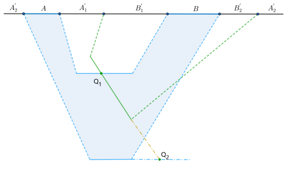
Comments: As rigorously said by Wen:2021qgx the bulk modular flows exactly settle at the boundary when they approach the boundary, so there are no orbits in the bulk. Thus to really find a boundary and bulk correspondence through local modular flow method, we should choose a cut-off surface, see Figure 2. Then there is a degree of freedom in choosing which modular flow line in the chosen cut-off surface correspond to a specific modular flow line at the asymptotic boundary. This freedom not only can affect the bulk point of PEE correspondence, i.e., $\epsilon_{i}$ in Figure 2, but also can affect the shape of the line between boundary and bulk corresponding points. Wen:2018whg make a good proposal on how to fix this freedom in AdS₃/CFT₂, but how to fix this freedom in flat₃/BMSFT model is not clear. As a byproduct in this paper, we find there is a consistent way to fix the d.o.f. in flat case although the underlying physical reasons need further study. In any case, this is not the focus of this paper and the intersection of RT like surfaces way turn out to be more general and less uncertain.

In 3D pure Einstein gravity, there is no propagating degree of freedom. The only way to construct different solutions is by taking quotient. Like the BTZ black holes are the discrete quotient manifolds of global AdS₃, the above mentioned zero mode backgrounds, i.e., the $M=0,J=0$ (the Poincaré vacuum), $M>0$ (FSC) and $M<0$ (including global Minkowski) zero mode backgrounds, are also the discrete quotient manifolds of global flat₃.

For each case we first give the coordinate transformations Apolo:2020bld that map that zero mode background to the global flat3 with coordinates $(t,x,y)$, then point out the corresponding boundaries or horizons of these quotient manifolds.

• •

  The Poincaré vacuum The coordinate transformations ²²2Note the transformations here are different with Apolo:2020bld ; Jiang:2017ecm , which depend on the boundary interval ${\cal A}$. are,

  $$t=\frac{(\alpha^{2}+4z^{2})r}{4\alpha}+\frac{2u}{\alpha},\quad x=zr+\frac{\beta}{\alpha},\quad y=\frac{(\alpha^{2}-4z^{2})r}{4\alpha}-\frac{2u}{\alpha}$$

  (3.6)

  for any value of $\alpha$ and $\beta$. Without loss of generality we choose $\alpha=1,\beta=0$ in this paper. In order to see the boundary of spacetime clearly, we need an inverse coordinate transformations

  $$u=\frac{t^{2}-x^{2}-y^{2}}{4(t+y)},\quad r=2(t+y),\quad z=\frac{x}{2(t+y)}.$$

  (3.7)

  So the Poincaré vacuum cover only the $t+y\geq 0$ part of the global Minkowski spacetime, see Figure 3 .

• •

  $M<0$ zero mode backgrounds The coordinate transformations are:

  		$\displaystyle t=\frac{1}{\sqrt{-M}}\left(r-Mu-\sqrt{-M}r_{c}\phi\right)$		(3.8)
  		$\displaystyle x=\frac{1}{\sqrt{-M}}\left[r\cos{\sqrt{-M}\phi}-r_{c}\sin{\sqrt{-M}\phi}\right]$
  		$\displaystyle y=\frac{1}{\sqrt{-M}}\left[r\sin{\sqrt{-M}\phi}-r_{c}\cos{\sqrt{-M}\phi}\right]$

  So we have the relation $x^{2}+y^{2}=(r^{2}+r_{c}^{2})/(-M)$, which leads to the boundary location $x^{2}+y^{2}=2r_{c}^{2}/(-M)$, See Figure 3. Note that if we have $J=r_{c}=0$, i.e., the whole Minkowski spacetime, then the codimension one boundary in Figure 3 would shrink to one dimensional line with $x=0,y=0$ excluding nothing from the global flat3 and consistent with the expectation.

• •

  $M>0$ zero mode backgrounds The coordinate transformations are:

  	$\displaystyle u=$	$\displaystyle\frac{1}{M}\left(r-\sqrt{M}y-\sqrt{M}r_{c}\phi\right),\quad r=\pm\sqrt{M(t^{2}-x^{2})+r_{c}^{2}}$
  		$\displaystyle\phi=-\frac{1}{M}\log{\left[\frac{\sqrt{M}(t-x)}{r+r_{c}}\right]}=\frac{1}{M}\log{\left[\frac{\sqrt{M}(t+x)}{r-r_{c}}\right]}$		(3.9)

  The spacetime region with $r>r_{c}$ exterior to Cauchy horizon locating at $r=r_{c}$ cover the parameter range

  $$t-x>0,\quad\quad t+x>0,$$

  (3.10)

  while the interior of the Cauchy horizon $0<r<r_{c}$ cover the parameter range

  $$t-x>0,\quad\quad t+x<0.$$

  (3.11)

  In Figure 3, the exterior of Cauchy horizon is above both the green and blue surfaces, and the interior of Cauchy horizon is the right part of the region enclosed by both the green and blue surfaces.

Note that if we draw the swing surface in the above compact Penrose diagrams, the finite bench would always penetrate the boundaries or horizons of the original spacetime. This curious phenomena is discussed in the last section.

The order of taking the infinite limit is a subtle issue in mathematics. Here is a good example due to the infinite range of both $r$ and $u$ coordinates in Bondi gauge. For the above coordinate transformations, if we take the limit $r>|u|\to\infty$ of Bondi coordinate, which is equivalent to keep coordinate $u$ a finite but arbitrary value and taking $r$ to infinity, the BMS field theory would always live on the future null infinity $\mathscr{I}^{+}$ for all $M=0$, $M>0$ and $M<0$ cases. However, we know that the global Minkowski spacetime with $M=-1,J=0$ contain not only the future null infinity $\mathscr{I}^{+}$ but also the past null infinity $\mathscr{I}^{-}$, which actually comes from another limit ³³3For simplicity in this subsection, we omit the mathematical proof of the statements, which can be obtained by following the same route as (4.11) and (4.18). $u<-r\to-\infty$. With the above observation, we explore the following limits

$$1).\;\;u<-r\to-\infty,\quad\quad 2).\;\;u>r\to\infty$$

(3.12)

in $M=0$, $M>0$ and $M<0$ solutions separately and summarize the new phenomena.

• •

  For the usual $r>|u|\to\infty$ limit, we have the expected Penrose diagram as 4 for all the zero mode solutions.

• •

  The Poincaré vacuum New phenomena only happen in the first limit of (3.12). As shown in 4, the $u<-r$ part of the boundary $\partial D[{\cal A}]$ of causal domain $D[{\cal A}]$ go around the spacelike infinity $i^{0}$ making now the boundary $\partial D[{\cal A}]$ a closed curve.

• •

  $M>0$ zero mode backgrounds New phenomena happen in both limits of (3.12). When $u<-r$ the $\partial D[{\cal A}]$ go around the spacelike infinity $i^{0}$ as in the case of the Poincaré vacuum; when $u>r$ the $\partial D[{\cal A}]$ go through the timelike infinity $i^{+}$, see 4, to a similar configuration symmetric about $\Phi=\frac{\pi}{2}$ axis. Thus the causal domain $D[{\cal A}]$ contains two disconnected parts, which is quite unusual.

• •

  $M<0$ zero mode backgrounds New phenomena happen only in the first limit of (3.12). As shown in 4, the $u<-r$ part of the $\partial D[{\cal A}]$ would plot a similar configuration on past null infinity $\mathscr{I}^{-}$ as the one on future null infinity $\mathscr{I}^{+}$. This is the only case that the field theory can touch $\mathscr{I}^{-}$ which is consistent with boundary of zero mode backgrounds in the last subsection.

If we consider the configurations of boundary interval ${\cal A}$ or the corresponding swing surface $\gamma_{{\cal A}}$ in the unusual limits (3.12), they are the limiting ones of the usual cases and do not affect our main conclusions.

We already observed that the entanglement entropy can be negative (2.19) in flat₃/BMSFT model. From the BMS field theory point of view, the reason and meaning of negative entanglement entropy need further solid explorations. However from the Einstein gravity point of view, the negative holographic entanglement entropy is already annoying enough and may ruin the correspondence of swing surface proposal. In this subsection, we give the mathematical derivation of negative sign of holographic entanglement entropy by identifying the entanglement entropy as a Noether surface charge ⁴⁴4Thank Wei Song for pointing out this viewpoint to us and Boyang Yu for early cooperation on this subsection. and explicitly using the swing surface construction. Also we would give the physical intuition about why the situations in flat₃/BMSFT model are different from the ones in AdS/CFT.

The holographic entanglement entropy can be viewed as an Noether surface charge evaluated along the HRT surface in AdS/CFT Faulkner:2013ica ,

$${\cal S}_{{\cal A}}={\cal Q}_{\xi}^{\gamma_{{\cal A}}}=-\frac{1}{16\pi G}\int_{\text{HRT}}\nabla^{\mu}\xi^{\nu}\epsilon_{\mu\nu\rho}dx^{\rho}=-\frac{1}{8}\int_{\text{HRT}}n^{\mu\nu}\epsilon_{\mu\nu\rho}dx^{\rho}$$

(3.13)

where $dx^{\rho}$ denotes the unit vector along the HRT surface, and $\xi^{\nu}$ denotes the bulk modular flow vector. We used the fact (2.26) in the third equality. The surface charge (3.13) is actually a line integral in 3D bulk, and to do the computation we should embed it into a specific coordinate system. Take the Poincaré coordinate of AdS/CFT as an example. If we fix the sign of $\epsilon_{txy}=1$ in Poincaré coordinates $(t,x,y)$ and integrate from the left endpoint of interval ${\cal A}$ to the right one, we would always have the following formulas

$$n^{\mu\nu}\epsilon_{\mu\nu\rho}\lvert_{\gamma_{{\cal A}}}=-2\hat{e}_{\rho},\quad{\cal Q}_{\xi}^{\gamma_{{\cal A}}}=\frac{1}{4G}\int_{left}^{right}\hat{e}_{\rho}dx^{\rho}=\frac{\text{Area}(\gamma_{{\cal A}})}{4G}.$$

(3.14)

In CFT the modular flow of a general boundary interval always have positive component along the positive direction of ordinate. While in BMS₃ field theory when fixing the abscissa, we can change the $u$ coordinate of the boundary interval to change the relative sign of the modular flow to the positive direction of ordinate. This global degree of freedom of boundary interval in flat₃/BMSFT model is the key to understand the negative sign of holographic entanglement entropy. Mathematically, using (4.49) we can get the parametrization equations of the bifurcating surface in Bondi coordinates of the Poincaré vacuum ⁵⁵5Note there are typos in (3.38) and (3.39) of Apolo:2020bld .

$$u(z)=\frac{-u_{r}(z-z_{l})^{2}+u_{l}(z-z_{r})^{2}}{(z_{l}-z_{r})(2z-z_{l}-z_{r})},\quad r(z)=-\frac{2(u_{l}-u_{r})}{(z_{l}-z_{r})(2z-z_{l}-z_{r})}$$

(3.15)

then the normalized directional vector $dx^{\rho}$ along the bench can be obtained as

$$dx^{\rho}=\text{sign}(u_{l}-u_{r})\left(\frac{(z-z_{l})(z-z_{r})}{z_{l}-z_{r}},\frac{2}{z_{l}-z_{r}},\frac{(z_{l}+z_{r}-2z)^{2}}{u_{l}-u_{r}}\right)$$

(3.16)

where we can see explicitly the sign of $dx^{\rho}$ depend on the relative value of $u_{l},u_{r}$ when we fix the values of $z_{l}$,$z_{r}$. The vector $\nabla^{\mu}\xi^{\nu}\epsilon_{\mu\nu\rho}$ can also be computed using (4.49)

$$\hat{e}_{\rho}=\nabla^{\mu}\xi^{\nu}\epsilon_{\mu\nu\rho}=\left(\frac{8\pi}{z_{l}-z_{r}},\frac{4\pi(z-z_{l})(z-z_{r})}{z_{l}-z_{r}},-\frac{8\pi(u_{l}-u_{r})}{(z_{l}-z_{r})^{2}}\right)$$

(3.17)

thus we have

$${\cal Q}_{\xi}^{\gamma_{{\cal A}}}=\frac{1}{4G}\int_{z_{l}}^{z_{r}}\hat{e}_{\rho}dx^{\rho}=\text{sign}(u_{l}-u_{r})\frac{\text{Area}(\gamma_{{\cal A}})}{4G}$$

(3.18)

which is indeed the expected form of holographic entanglement entropy in the Poincaré vacuum of the flat₃/BMSFT model Apolo:2020qjm ,

$${\cal S}_{{\cal A}}=\frac{u_{lr}}{2Gz_{lr}}=\text{sign}(u_{l}-u_{r})\frac{|2l_{u}|}{4Gl_{z}}={\cal Q}_{\xi}^{\gamma_{{\cal A}}}$$

(3.19)

where $u_{lr}=u_{l}-u_{r}$ and $z_{lr}=z_{l}-z_{r}$.

We emphasize that not only the entanglement entropy Apolo:2020bld , but also the reflected entropy Basak:2022cjs , entanglement negativity Basu:2021awn and PEE in flat₃/BMSFT model all can be negative. These key observations imply us that this is actually a general character of flat₃/BMSFT model. Although for the mixed state entanglement measures we do not have a local modular flow to mathematically prove the above statement.

In flat₃/BMSFT model the bulk theory is pure Einstein gravity, however we need other property of swing surface to match the expectation of being holographic entanglement entropy and have to consult to the Noether charge formalism. This is unusual to what we learned in AdS/CFT. We leave the discussion in the last section.

Due to the phenomena that swing surface always penetrate the boundary or horizon of the original spacetime, in the following we explore the causality structure in global flat₃ and overlook the quotient manifolds stuff momentarily. In order to specify which bulk region in global flat₃ have similar properties of entanglement wedge ${\cal W}_{{\cal E}}[{\cal A}]$ in AdS/CFT holography, we are facing two unavoidable questions. The first one is whether this region is a closed co-dimension zero bulk region. The other one is which part of the bifurcating surface is more fundamental, or at least more useful, the finite bench $\gamma$ or the infinite bifurcating surface $\gamma_{\xi}$.

Due to the non-local property in $u$ direction of boundary BMS field theory, which can be seen from the two point correlation function (2.12), it’s rather unclear that a closed bulk region related to the swing surface $\gamma_{{\cal A}}$ would exist. One example is the AdS₃/WCFT holographic model, the ”pre-entanglement wedge” is not closed in the $v$ direction due to the non-local feature in $z$ direction of boundary WCFT Chen:2022fte .

Related to the second question, there are two special bulk surfaces that we could grow null normal congruence from to construct the boundaries of a bulk region. One is the whole bifurcating surface $\gamma_{\xi}$ which is unbounded and invariant under the bulk modular flow $\xi$. Another one is the finite bench $\gamma$ which is a bounded portion of $\gamma_{\xi}$. Due to the homology condition between swing surface and boundary interval as well as the Noether charge formalism (3.13), the finite bench $\gamma$ may be more basic.

The above mentioned questions turn out to be closely related to each other in flat₃/BMSFT model. We approach these problems from more practical ways rather than the more philosophical homology condition. To be consistent with the presentation style of this section, we just show the observations.

The existing literature Basak:2022cjs ; Basu:2021awn only consider the symmetric two intervals on the boundary, where the EWCS would end on the finite bench $\gamma$. However when considering more general configurations of boundary two intervals, we observed that the endpoints of EWCS can exceed $\gamma$. We plot several new situations in Figure 5, where the usual expected entanglement wedge Apolo:2020bld ; Basak:2022cjs and true EWCS are plotted. We can see from the pictures that the not carefully defined connected entanglement wedge would lead to big problems.

Due to these observations, we see that the whole modular invariant bifurcating horizon $\gamma_{\xi}$ may be more basic. We would provide more evidence along this perspective through PEE, BPE and bulk modular flow in the next section.

There are several coordinate systems that we would go back and forth when trying to clearly show the causal relations between boundary field theory and bulk gravity theory.

• •

  Bondi coordinates of the original Poincare vacuum:

  $$\text{bulk}:(u,r,z),\quad\text{boundary}:(u,r\to\infty,z)$$

  (4.7)

• •

  Cartesian coordinates and Penrose coordinates of the covering global Minkowski spacetime:

  $$\text{Cartesian}:(t,x,y),\quad\text{Penrose}:(U,V,\Phi),\;(T,X,Y)$$

  (4.8)

  which are related by the standard textbook transformations,

  $$U=\arctan{(t-\sqrt{x^{2}+y^{2}})},\quad V=\arctan{(t+\sqrt{x^{2}+y^{2}})},\quad\Phi=\phi=\arctan{\frac{y}{x}}$$

  $$T=V+U,\quad X=(V-U)\cos{\Phi},\quad Y=(V-U)\sin{\Phi}$$

  (4.9)

From boundary to boundary

we first deal with the image of field interval ${\cal A}$ on the future null infinity $\mathscr{I}^{+}$ ⁶⁶6This is a choice of us, which means that we can also choose to map boundary field theory to the past null infinity $\mathscr{I}^{-}$ by putting minus signs in coordinate transformations (3.6). of Penrose diagram with coordinates $(U,V,\Phi)$. There are several facts about this map:

• •

  constant $z$ line of field theory would be mapped to constant $\Phi$ line on $\mathscr{I}^{+}$ of the Penrose diagram. So a strip like region which is the causal domain $D[{\cal A}]$ of field interval would map to a corner region on the boundary null cone. In particular, the $z=0$ axis would be mapped to $\Phi=\frac{\pi}{2}$ line. This can be seen from the following transformation,

  $$\Phi=\arctan{\frac{y}{x}}|_{r\to\pm\infty}=\arctan{\frac{1-4z^{2}}{4z}}.$$

  (4.10)

  When $z$ goes from $0$ to $\infty$, $\Phi$ would go from $\frac{\pi}{2}$ to $-\frac{\pi}{2}$. Because (4.10) is a monotonic decreasing function when $z>0$, then the map is one to one.

• •

  A symmetric interval about the origin $(u=0,z=0)$ would map to a symmetric interval about the point $(U=0,V=\frac{\pi}{2},\Phi=\frac{\pi}{2})$ on $\mathscr{I}^{+}$ of the Penrose diagram. This can be seen as follows:

  	$\displaystyle\sqrt{x^{2}+y^{2}}|_{r\to\pm\infty}=\frac{1}{4}(1+4z^{2})|r|+\frac{2u(1-4z^{2})}{1+4z^{2}}\frac{|r|}{r},$
  	$\displaystyle\text{when}\;r\to\infty,\quad U=\arctan{\frac{4u}{1+4z^{2}}},\quad V=\frac{\pi}{2}.$		(4.11)

  (4.10) and (4.11) give us a bijective map from the infinite $(u,z)$ plane where the original BMS field theory live to the whole future null infinity $\mathscr{I}^{+}$ of the compact Penrose diagram.