Review of proton and nuclear shape fluctuations at high energy
Abstract
Determining the inner structure of protons and nuclei in terms of their fundamental constituents has been one of the main tasks of high energy nuclear and particle physics experiments. This quest started as a mapping of the (average) parton densities as a function of longitudinal momentum fraction and resolution scale. Recently, the field has progressed to more differential imaging, where one important development is the description of the event-by-event quantum fluctuations in the wave function of the colliding hadron.
In this Review, recent developments on the extraction of proton and nuclear transverse geometry with event-by-event fluctuations from collider experiments at high energy is presented. The importance of this fundamentally interesting physics in other collider experiments like in studies of the properties of the Quark Gluon Plasma is also illustrated.
I Introduction
Determining the structure of protons and nuclei in terms of their fundamental constituents and their mutual interactions is one of the long term quests in particle physics. In the last decades, more and more detailed pictures of the (especially) proton structure have been obtained. The most important input for these studies is provided by deep inelastic scattering (DIS) experiments, in which simple pointlike leptons are used to probe the proton substructure. Traditionally, the partonic structure of the proton is presented in terms of the parton distribution functions that describe the quark and gluon densities as a function of longitudinal momentum fraction of the proton carried by the parton. In particular, thanks to the large amount of precise deep inelastic scattering data from HERA Aaron:2009aa ; Abramowicz:2015mha , the quark and gluon distribution functions for the proton are known down to low with good precision.
Beyond the one dimensional distributions (that depend on the longitudinal momentum fraction), it is fundamentally interesting to reveal the geometric structure of proton. In addition to the average size and shape, also the shape fluctuations are basic properties of the proton and should be determined. This knowledge is also crucial for the proper interpretation of many other experimental measurements. The average spatial distribution of partons is encoded in the generalized parton distribution functions Mueller:1998fv ; Ji:1996nm ; Radyushkin:1997ki ; Collins:1996fb . In this Review, however, a step beyond these distributions is taken and the event-by-event fluctuations of the proton (and nuclear) shape are considered, concentrating on the gluonic structure at small .
There are two different venues that have been recently used to access the geometric shape and shape fluctuations. One can look at particle correlations in high multiplicity collisions generated by the (possible) hydrodynamical response to the initial state spatial anisotropies. In heavy ion collisions, collective phenomena have been used to show the formation fo the Quark Gluon Plasma, and to determine its fundamental properties. In heavy ion collisions the geometry is dominated by the shapes of the colliding nuclei, and the effects sensitive to the nucleon shape (and shape fluctuations) are less important. In proton-lead and proton-proton collisions the initial state geometry is controlled by the single proton, and the shape fluctuations can potentially be observed more clearly assuming that a hydrodynamically evolving fluid is produced. However, the applicability of hydrodynamics when describing such a small systems produced in proton-proton or proton-lead collisions is not completely established and is currently under an intensive research.
An another approach is to look at observables that directly probe the event-by-event fluctuations in the target wave function. As will be discussed in detail in this Review, one of these processes is incoherent diffraction in deep inelastic scattering. In these events, the target proton or nucleus dissociates and a rapidity gap exists between the target remnants and the diffractively produced system (e.g. a vector meson). In addition, one can consider fully elastic scattering processes to obtain more indirect evidence of the proton shape fluctuations.
In this review the focus in on the proton and nuclear shape fluctuations at high energy (small momentum fraction ). In Sec. II it is shown how diffractive processes can be used to constrain the average shape of the target, as well as probe the event-by-event fluctuations at different distance scales. A theoretical framework used to describe these high energy processes based on the Color Glass Condensate effective theory of QCD is shortly introduced in Sec. III. Based on this discussion, in Sec. IV we review the recent progress in using the diffractive vector meson production to constrain the proton shape fluctuations. Elastic proton-proton scattering, and particle correlations in high-multiplicity proton-proton collisions, are discussed in the context of fluctuating proton structure in Sec. V. Fluctuating nucleons in nuclei in the context of diffractive vector meson production and hydrodynamical simulations of the Quark Gluon Plasma production in proton-lead collisions are reviewed in Sec. VI.
II Exclusive scattering as a probe of transverse geometry
As discussed above, the total cross section in DIS can be studied to measure the total partonic densities in protons and nuclei. To obtain a more detailed picture of the target, more differential observables are needed. One especially powerful process is exclusive production of a vector meson with the same quantum numbers as the photon in deep inelastic scattering:
| (1) |
Here refers to a vector meson (), and the target can be a proton or a nucleus . An experimental signature is a rapidity gap (empty detector) between the produced vector meson and the target. The target can either remain in the same quantum state or dissociate, these processes will be later considered separately. In general, these processes are called diffractive.
There are two main advantages that make vector meson production powerful. First, in order to produce the vector meson and nothing else, there can not be a net color charge transfer to the target. This requires at least two gluons to be exchanged with the target, and the cross section consequently scales approximatively as the gluon density squared Ryskin:1992ui . The other advantage is that only in the exclusive scattering process it is possible to measure the total momentum transfer , and interpret that as the Fourier conjugate to the impact parameter. Consequently, these processes probe not only the density of partons, but also their spatial distribution.
Let us first consider coherent diffraction, in which the target remains in the same quantum state after the interaction. In this case, the cross section is calculated by applying the Good-Walker formalism Good:1960ba , which states that the cross section is determined by the average interaction of the states that diagonalize the scattering matrix with the target. At high energies, these states are the Fock states of the incoming virtual photon with a fixed number of partons (at leading order a quark-antiquark pair) at fixed transverse coordinates, probing a fixed configuration of the target. This formalism can then be generalized to also include fluctuating target configuration. The cross section then reads Miettinen:1978jb (following the notation of Ref. Kowalski:2006hc )
| (2) |
where refers to the target proton or nucleus, is the squared four momentum transfer (at high energies ) and is the amplitude for the diffractive scattering (the same amplitude also enters in the calculation where the target dissociates, as demonstrated shortly). As the average is taken over all possible configurations of the incoming proton or nucleus, the scattering amplitude is sensitive to the average interaction of the quark dipole with the target. This, in turn, is controlled by the average distribution of small- gluons in the target wave function. Thus, the coherent cross section generally probes the average structure of the target. We will return to the calculation of later in Sec. III.
Let us then consider the class of events in which the outgoing proton or nucleus is not in the same quantum state as the incoming particle following Ref. Caldwell:2009ke . These events are called incoherent, and the experimental manifestation is that the target dissociates into a system of particles, maintaining the rapidity gap to the produced vector meson. To describe these events, the scattering amplitude in the case where initial state is and the final state is is expressed as (we use a shorthand notation to refer to the diffractive scattering amplitude ). The initial and final states are required to be different. The squared transition amplitude, which enters in the cross section, reads
| (3) |
To get the last line the completeness of states, , is used. Note that the sum over final states includes all possible states for the final state proton, and not only the different spatial configurations of its ground state. To get the cross section, the squared amplitude must be averaged over the possible initial states . The first term in Eq. (3) then becomes the squared diffractive scattering amplitude averaged over the initial configurations, and the second term gives the average of the diffractive scattering amplitude squared. The resulting incoherent cross section then reads
| (4) |
Here denotes the final state proton or nucleus in a state which differs from the initial state. Due to the different ordering of the squaring and averaging of the amplitude , the incoherent cross section measures how much the scattering amplitude fluctuates between the different possible initial state configurations. Because the total momentum transfer is measurable and the Fourier conjugate to the impact parameter, this property can be used to constrain the geometry fluctuations in the target at different length scales as demonstrated shortly. When applying Eq. (4) away from where it is strictly applicable Frankfurt:1994hf ( being the target size), a specific model for the fluctuating structure in the transverse plane is needed, as originally presented in Ref. Miettinen:1978jb . Additionally, one has to assume that the non-zero momentum transfer does not mix the states with different transverse structure that are used to diagonalize the scattering matrix. Up to how large this extension is valid is not yet completely determined.
An analogous process to the exclusive vector meson production is deeply virtual compton scattering (DVCS), in which a real photon is produced. At high energies where the target is dominated by gluons, the DVCS process is also sensitive to the small- gluons and their spatial distribution in the target. The difference to the exclusive vector meson production is that one does not need to model the non-perturbative vector meson formation process, and the mass of the meson does not provide a hard perturbative scale. On the other hand, one can also work in terms of the generalized parton distribution functions or GPDs (see Ref. Diehl:2003ny for a review), that depend both on the longitudinal momentum fraction and transverse coordinate. For the possibilities to use DVCS to constrain the quark and gluon GPDs in the future Electron-Ion Collider, see e.g. Ref. Accardi:2012qut .
To summarize, the diffractive processes provide unique constraints on the target structure. First, the coherent cross section measures the average parton distribution. In exclusive scattering where the impact parameter dependence is probed, coherent vector meson production gives access to the spatial distribution of small- partons (dominantly gluons). Simultaneously, incoherent vector meson production where the target dissociates measures the degree of fluctuations in the scattering amplitude (at the length scale controlled by the inverse momentum transfer) is measured. In Sec. IV it is show how the proton geometry fluctuations can be obtained by applying these two constrains simultaneously111In these analyses no constraints on the impact parameter are imposed. However, as proposed in Ref. Lappi:2014foa , it may also be possible to analyze incoherent diffraction at different centrality classes..
III Dipoles probing protons and nuclei at high energy

At high energies, the lifetime of the quark-antiquark fluctuation is much longer than the timescale of the dipole-target interaction. Consequently, the production cross section factorizes, and it becomes natural to describe the scattering processes in the dipole picture Mueller:1993rr ; Nikolaev:1991et . First, the incoming photon splits to a quark-antiquark dipole, which is a simple QED process Kovchegov:2012mbw . Subsequently, the dipole scatters elastically off the target. Long after the interaction, non-perturbative vector meson formation from the quark dipole takes place. This factorization makes it possible to write the diffractive scattering amplitude in the Color Glass Condensate framework (for a review, see e.g. Refs. Iancu:2003xm ; Gelis:2010nm ; Albacete:2014fwa ; Blaizot:2016qgz ) as Kowalski:2006hc
| (5) |
illustrated in Fig. 1. Here, the virtual photon wave function describes the photon to dipole splitting, and its overlap with the vector meson wave function controls the contribution of different dipole sizes and longitudinal momentum fractions at fixed virtuality . The dipole-target scattering is described by the dipole amplitude , which depends on the particular configuration of the target . The transverse momentum transfer is the Fourier conjugate to the impact parameter (center of the dipole) as discussed earlier, with the correction taking into account that the vector meson wave function is not taken in the forward kinematics Bartels:2003yj 222It has recently been argued in Ref. Hatta:2017cte that the conjugate to the momentum transfer should be , instead of . However, numerical results are almost identical in both cases.. The target structure is probed at the longitudinal momentum fraction
| (6) |
which is analogous to the Bjorken- of DIS. Here is the center-of-mass energy for the photon-nucleon scattering, the vector meson mass, the photon virtuality and the nucleon mass.
The connection to the transverse geometry is apparent in Eq. (5), as the dipole-target scattering amplitude is Fourier transformed from the coordinate space to the momentum space. When the coherent cross section is calculated, one first takes the average of over different target configurations. This averaging results in average dipole-target scattering amplitude . As the dipole amplitude is approximatively proportonal to the gluon density at the given impact parameter , the distribution of the coherent cross section is approximatively the 2-dimensional Fourier transform of the spatial gluon distribution. The extraction of the impact parameter dependence of the dipole amplitude was discussed for the first time in Ref. Munier:2001nr (see also Ref. Ralston:2001xs ), inspired by the determination of the proton density profile based on elastic proton-proton collision measurements presented in Ref. Amaldi:1979kd .
It is customary to include two corrections in phenomenological studies of exclusive vector meson production following Ref. Kowalski:2006hc . First, one usually assumes that the dipole amplitude is purely real and consequently the vector meson production amplitude (5) imaginary. By requiring that the scattering amplitude is an analytical complex function, the real part can be recovered and included as a numerically small (generally at the cross section level) correction. Additionally, the so called skewedness correction which takes into account the fact that in the two-gluon exchange limit the two gluons carry a different fraction of the target longitudinal momentum Shuvaev:1999ce . This correction is numerically large (generically up to , see e.g. Ref. Mantysaari:2017dwh ), and its applicability in the dipole picture discussed here where the two quarks undergo multiple scattering in the target color field is not completely established.
A major advantage of the CGC approach is that both inclusive and diffractive observables can be described in the same framework in terms of same degrees of freedom. This is not the case in collinear factorization approach, as the parton distribution functions are by definition inclusive, and relating them to exclusive processes is not straightforward (see however Guzey:2013qza ). In CGC, the QCD dynamics is described in terms of the dipole-target scattering amplitude which includes all information about the target structure. As an illustration, let us consider Eq. (5) in the case where the final state is a virtual photon, and write where is the photon wave function. Now, the optical theorem states that the total photon-proton cross section is related to the imaginary part of the forward scattering amplitude (). As the dipole amplitude is generally assumed to be real and the cross section is obtained by averaging over all possible target configurations, the total photon-proton (or photon-nucleus) cross section becomes
| (7) |
We immediately note that unlike diffractive cross sections, inclusive cross section entering e.g. in the structure functions is only sensitive to the gluon density integrated over the whole target. As such, it can not distinguish between different impact parameter distributions of the same overall gluon density. In general, determining the collision centrality in deep inelastic scattering is challenging, see however Ref. Zheng:2014cha where the forward neutron multiplicity is proposed to act as a proxy for the centrality in the future Electron Ion Collider.
In the Color Glass Condensate framework, the dipole-target scattering amplitude satisfies perturbative evolution equations, such as the JIMWLK JalilianMarian:1996xn ; JalilianMarian:1997jx ; JalilianMarian:1997gr ; Iancu:2001md equation (named aver Jalilian-Marian, Iancu, McLerran, Weigert, Leonidov and Kovner). This equation, or its NLO version Balitsky:2013fea ; Kovner:2013ona , is equivalent to the infinite hierarchy or coupled differential equations known as the Balitsky hierarchy, which reduces to a closed equation in the mean field and large- limit, known as the Balitsky-Kovchegov (BK) equation Kovchegov:1999yj ; Balitsky:1995ub also available at the NLO accuracy Balitsky:2008zza ; Balitsky:2013fea . The initial condition, describing e.g. the dipole amplitude at the initial Bjorken-, is a non-perturbative input to the evolution and is usually obtained by fitting the HERA deep inelastic scattering data as in Refs. Albacete:2010sy ; Lappi:2013zma ; Ducloue:2019jmy . A challenge in this approach is to describe the evolution of the target geometry, as the perturbative evolution equations produce long-distance Coulomb tails that result in cross sections growing much faster than seen in the measurements. This growth should be tamed by confinement scale effects, whose implementation is challenging, see e.g. Berger:2011ew ; Mantysaari:2018zdd . Consequently, in phenomenological applications one often applies parametrizations for the dipole amplitude that include dependence on the proton geometry, and are matched to perturbative QCD in the dilute region. A common choice is the IPsat parametrization Kowalski:2003hm with free parameters fitted to HERA data in Rezaeian:2012ji ; Mantysaari:2018nng . In this parametrization the dipole amplitude is written as
| (8) |
with
| (9) |
Here is the proton density profile with possible event-by-event fluctuations (normalized such that ), and the gluon distribution which satisfies the DGLAP equation Gribov:1972ri ; Gribov:1972rt ; Altarelli:1977zs ; Dokshitzer:1977sg to guarantee a smooth matching to perturbative QCD at small dipoles corresponding to the dilute region.
Finally, to conclude this Section let us briefly mention the connection to the collinear factorization. In the non-relativistic limit, where the quark and antiquark carry the same longitudinal momentum () and when the multiple interactions with the target are neglected, one recovers the so called Ryskin result Ryskin:1992ui for the coherent cross section as shown explicitly in Ref. Anand:2018zle :
| (10) |
In this form the sensitivity on the small- gluons is apparent, as the cross section is proportional to the squared gluon density (although the skewedness correction discussed above could be applied), and the dependence is parametrized in terms of the target form factor . However, this simple treatment neglects the fact that the inclusive structure functions can not be directly used when describing exclusive processes. Here is the leptonic decay width of the vector meson having mass , and the momentum scale of the process.
IV Proton structure fluctuations from diffraction
IV.1 Constraining the fluctuations at small
In Sec. II it was discussed how the coherent cross section is sensitive to the average structure of the target, and how the incoherent cross section measures the amount of event-by-event fluctuations. In this section, the recent progress in constraining the fluctuating transverse geometry of the proton based on HERA vector meson production data is reviewed.
Coherent and incoherent vector meson production has been extensively measured at HERA (where the incoherent process is usually called proton dissociation), where electrons and positrons were collided with protons at center-of-mass energy . This translates into photon-proton center-of-mass energies in the range . Both H1 and ZEUS measured diffractive production in the photoproduction () and electroproduction () regions Breitweg:1999jy ; Chekanov:2002xi ; Aktas:2003zi ; Chekanov:2004mw ; Aktas:2005xu ; Chekanov:2009ab ; Alexa:2013xxa . In addition to , exclusive production of lighter Adloff:1999kg ; Aid:1996ee ; Chekanov:2007zr ; Aaron:2009xp and Chekanov:2005cqa ; Aaron:2009xp mesons as well as heavier upsilons Breitweg:1998ki ; Chekanov:2009zz ; Adloff:2000vm has also been measured.
The possibility to constrain the event-by-event fluctuations in the proton was pioneered in Ref. Mantysaari:2016ykx based on ideas discussed in Refs. Miettinen:1978jb ; Caldwell:2009ke , first by using the IPsat parametrization, Eq. (8), to describe the dipole-proton interaction. In this case, if there are no fluctuations in the proton density profile , the incoherent cross section (4) vanishes. On the other hand, the coherent spectrum is sensitive to the proton profile. As the mass of the vector meson suppresses contributions from large dipoles , one can approximatively linearize the IPsat dipole (8), substitute that to the diffractive scattering amplitude (5) and obtain an estimate for the dependence of the coherent cross section:
| (11) |
when the proton density profile is assumed to be Gaussian:
| (12) |
Thus, the slope directly measures the size of the proton: the transverse proton radius is . In practice, as the impact parameter profile is more complicated in the IPsat parametrization, the Fourier transform results in diffractive minima at large (outside the range where H1 and ZEUS were able to measure the spectra), see discussion in Ref. Armesto:2014sma . This is a general feature in diffractive scattering, and the location of the first minimum is controlled by the size of the target as .
To obtain also a non-zero incoherent cross section, the proton density profile was taken to have event-by-event fluctuations in Ref. Mantysaari:2016ykx . The simplest ansatz, motivated by the picture where the three constituent quarks emit small- gluons around them, is to assume that the proton consists of hot spots at random locations (see also Ref. Mitchell:2016jio for a more detailed discussion of possible ways to sample constituent quark structure). In this case, the density profile is written as
| (13) |
In a simple case, inspired by the constituent quark model, one can take , but other choices are also possible Mantysaari:2016jaz ; Cepila:2016uku . The distances for the hot spots from the center of the proton are sampled from a Gaussian distribution whose width is a free parameter, as is the size of the hot spot . Requiring a simultaneous description of both coherent and incoherent production data, optimal values for these parameters can be determined.

Coherent and incoherent photoproduction () spectra computed using a spherical proton (in which case the incoherent cross section vanishes) and a fluctuating proton with the optimal parameters and from Ref. Mantysaari:2016jaz are shown in Fig. 2. Note that the Bjorken- probed here is approximatively . As the characteristic hot spot separation turns out to be much larger than the hot spot size , large spatial geometry fluctuations are needed to obtain a good fit to the HERA data. Although the structure fluctuations mostly affect the incoherent cross section (which would otherwise vanish in this calculation), the coherent cross section is also somewhat modified by the substructure fluctuations. As the coherent cross section is only sensitive to the average structure of the target, or to the average dipole-target scattering amplitude, it would also be possible in principle to construct a parametrization for the fluctuating proton structure which leaves the average dipole-target interaction intact. Note that Eq. (13) modifies the average proton shape, due to the non-linear dependence on the density function in the dipole amplitude (8). Consequently, the different results for the coherent cross section should not be taken to quantify the effect of proton shape fluctuations on coherent J/ production.
At large the slope of the incoherent spectrum is controlled by the size of the smallest object that fluctuates as shown explicitly in Ref. Lappi:2010dd . At small , on the other hand, one is sensitive to the fluctuations at long distance scale . With only geometry fluctuations included in the model, the small- part of the incoherent spectra is underestimated. To improve the description of the HERA data, in Ref. Mantysaari:2016ykx additional density fluctuations were implemented following Ref. McLerran:2015qxa , by allowing the density of each of the hot spots to fluctuate independently. As can be seen in Fig. 2, when the density (labeled as ) fluctuations are included on top of geometry fluctuations, an improved description of the HERA data is obtained at all .
It is crucial to note that the hot spot picture applied above is only one possible fluctuating density profile for the proton compatible with the HERA vector meson production data. The incoherent cross section measures how large fluctuations there are in the diffractive scattering amplitude, and the distance scale probed is set by . There are multiple different fluctuating geometries that result in the same variance. This was explicitly demonstrated in Ref. Mantysaari:2016jaz where instead of a hot spot structure, the proton density profile was constructed based on a lattice QCD inspired picture where the constituent quarks are connected via color flux tubes that merge at a specific point inside the proton Bissey:2006bz . Fixing again the free parameters, the tube width and the width of the distribution from which the constituent quark positions are sampled, it is possible to obtain an equally good description of the coherent and incoherent production data. This means that the average proton shape and the amount of fluctuations are approximatively the same as in the hot spot parametrization.
In addition to geometry and density fluctuations, one expects to have individual color charge fluctuations in the proton. To estimate their contribution to the incoherent cross section, one needs to go beyond the IPsat parametrization. One possible approach is to apply the McLerran-Venugopalan model in the CGC framework McLerran:1993ni . Here, the fluctuating color charges are included by assuming that the color charges are local random Gaussian variables, with the width of the distribution proportional to the local density, characterized by the saturation scale . The color charge density (where is the color index) in the MV model is thus sampled from a distribution
| (14) |
with the expectation value zero. The color charge density is taken to be directly proportional to the local saturation scale which can be extracted from the IPsat parametrization. The geometry and density fluctuations can thus be included by introducing them in the IPsat parametrization as discussed above.
In practice, in this approach one samples the color charges for each event, and then solves the classical Yang-Mills equations to obtain the Wilson lines at each point on the transverse plane. The Wilson lines describe the color rotation of a high energy quark when it propagates through the target at fixed transverse coordinate , and the dipole-target amplitude is obtained as a trace of two Wilson lines:
| (15) |
The color charge fluctuations result in a finite incoherent cross section even if no geometry fluctuations are introduced. However, this contribution is small (suppressed by ) Dominguez:2008aa ; Marquet:2009vs and in practice results in an incoherent cross section significantly underestimating the HERA data on photoproduction as shown by dashed lines in Fig. 3.
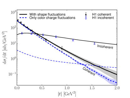
In Ref. Mantysaari:2016jaz , geometry and density fluctuations were added to the CGC framework described above. Using the hot spot geometry with three hot spots and fitting the hot spot size and their average separation it is possible to obtain an excellent description of the H1 photoproduction spectra as shown in Fig. 3 (solid lines). The resulting proton fluctuations (at corresponding to the kinematics of the H1 data) are illustrated in Fig. 4, where four examples of the sampled protons are shown. The proton density is illustrated by showing . Note that as individual Wilson lines are not gauge invariant (unlike ), this should be considered only as an illustration in arbitrary units. However, the conclusion is similar as in the simpler framework where the IPsat parametrization is used: large event-by-event fluctuations are needed to describe the incoherent vector meson data from HERA, even when the color charge fluctuations are included. Additionally, it is shown that by just introducing large overall density fluctuations it is not possible to obtain a correct incoherent spectrum Mantysaari:2016jaz .

This relatively simple geometry has been further developed in Ref. Traini:2018hxd using an explicit quark model calculation for the wave function of the valence quarks, where correlations between the constituent quarks have been taken into account. The spin dependence of the forces between the quarks results in both attractive and repulsive interactions. All parameters except the size of the small- gluon cloud around the valence quark can be fixed by the low energy proton and neutron structure data, and consequently only one parameter (size of the gluon cloud) needs to be adjusted to simultaneously describe the coherent and incoherent vector meson production data from HERA. The proton shape fluctuations extracted in Ref. Traini:2018hxd are very similar to the results summarized above.
IV.2 Energy dependence of the fluctuating structure
In the discussion above the proton shape fluctuations were constrained at fixed Bjorken-, without considering the dependence of the proton structure. On the other hand, there are clear measurements that show that the transverse size of the proton grows with decreasing . For example, when the slope of the coherent photoproduction cross section, see Eq. (11), is extracted at different center-of-mass energies (corresponding to different ), a clear logarithmic dependence on the energy is observed:
| (16) |
The parameters measured by H1 Aktas:2005xu are and .
In addition to the growing proton size, fluctuations should evolve in energy. At asymptotically large energies, where the black disc limit is excepted to be reached e.g. as a result of the small- evolution described in the Color Glass Condensate framework, the probability for the dipole to scatter saturates to unity, and there are no event-by-event fluctuations. In this limit, the incoherent cross section is expected to be suppressed, as event-by-event fluctuations are only possible at the dilute edge of the proton. The energy dependence of the coherent and incoherent cross section measured at HERA Alexa:2013xxa show that the incoherent-to-coherent cross section ratio decreases with increasing center-of-mass energy. Recently, the ALICE collaboration has studied photoproduction at different photon-proton center-of-mass energies TheALICE:2014dwa ; Acharya:2018jua in ultraperipheral collisions Bertulani:2005ru ; Klein:2019qfb . The energy dependence of the incoherent cross section is not measured so far, but the two muon (decay products of ) transverse momentum distributions are compatible with the incoherent cross section being suppressed compared to the coherent one at high energies.
In phenomenological calculations different approaches have been taken to describe the energy dependence of the fluctuations. In the framework developed in Ref. Cepila:2016uku and further applied in Refs. Cepila:2017nef ; Cepila:2018zky the proton is assumed to consist of hot spots, whose number depends on the Bjorken- as
| (17) |
This functional form is motivated by a generally used parametrization of the gluon distribution at the initial scale used in parton distribution function fits (see also Refs. Liou:2016mfr ; Domine:2018myf for a recent discussion of the gluon density fluctuations in dilute hadrons). The number of gluons is then related to the number of hot spots, and the locations for the hot spots are sampled randomly similarly as described in Sec. IV.1. The model parameters , and have been fixed by comparing to energy dependence of the incoherent photoproduction data form H1 Alexa:2013xxa . In this approach a good description of the energy dependence of both coherent and incoherent H1 data is obtained Cepila:2016uku .
A genuine prediction of this framework is that as the number of hot spots in a fixed transverse area increases, the event-by-event fluctuations will eventually disappear. This results in an incoherent cross section which has a maximum at the center-of-mass energy (in case of photoproduction), after which it decreases with increasing energy, as shown in Fig. 5. In ultraperipheral proton-lead collisions at the LHC, center of mass energies in the TeV range for the photon-proton system can be achieved. A future measurement of the energy dependence of the cross section ratio will be a crucial test for the model. However, as the proton size evolution is not included in this framework, the model would not reproduce the experimentally observed evolution of the slope of the coherent cross section shown in Eq. (16).

A different approach to the energy evolution was taken in Ref. Mantysaari:2018zdd , where the perturbative JIMWLK evolution equation describing the Bjorken- dependence was applied. There, using the Color Glass Condensate framework described above the proton fluctuating structure at initial Bjorken- was constrained by comparing with the production data at . On top of geometry fluctuations, also overall density fluctuations for each of the three hot spots sampled at initial are included. Then, the different proton configurations were separately evolved to smaller by solving the JIMWLK equation, and using the evolved protons the cross sections at higher center-of-mass energies were obtained.


The calculated incoherent-to-coherent cross section ratio as a function of photon-proton center-of mass energy is shown in Fig. 6. The decreasing ratio shows that the evolution washes out the initial hot-spot structure. This can be seen from the actual evolution of a one particular proton configuration illustrated in Fig. 7. The free parameters in the evolution, the value for the fixed QCD coupling constant and the infrared regulator limiting the unphysical growth of the proton size due to the missing confinement scale effects, are fixed by requiring a compatible evolution speed with the inclusive charm structure function data. However, a disadvantage of this approach is that the simultaneous description of both inclusive and exclusive observables is not possible without introduction of a non-perturbative contribution, due to the numerically large contributions from non-perturbatively large dipoles (see Mantysaari:2018nng for a detailed analysis of large dipole contributions).
V Proton shape from proton-proton collisions
So far it has been discussed how the proton shape fluctuations can be constrained based on exclusive vector meson production in deep inelastic scattering. Qualitatively similar results have been obtained based on analyses of other observables, and these findings support the picture developed above where the proton shape has large event-by-event fluctuations.
V.1 Elastic scattering
In Ref. Albacete:2016pmp elastic proton-proton scattering at small momentum transfer is studied. This process is measured at and center-of-mass energy at the LHC Antchev:2011zz ; Antchev:2018rec ; Antchev:2018edk (only data is used in the analysis of Ref. Albacete:2016pmp ), and at smaller at ISR Amaldi:1979kd . As there is no hard scale, perturbative calculations can not be applied to describe this process. Instead, the real and imaginary part of the scattering amplitude can be parametrized, and the values for the unknown parameters can be constrained by fitting the spectra and requiring that that the real-to-imaginary part ratio satisfies the measured value333In case of LHC, the authors use an extrapolated value from Cudell:2002xe which is compatible with the more recent TOTEM measurement (depending on physics assumptions) Antchev:2017yns ..
A striking observation in elastic scattering processes is the so called Hollowness or grayness effect Alkin:2014rfa ; Dremin:2015ujt ; Troshin:2016frs ; Arriola:2016bxa : the inelasticity density describing how different impact parameters contribute to the inelastic cross section has a maximum at a non-zero impact parameter at LHC energies444The hollowness effect could be seen to suggest that the black disk limit discussed in Sec. IV.2 it not necessarily reached at asymptotically high energies.. On the other hand, at lower ISR energies the maximum is at at ISR energies. The inelasticity density is defined in terms of the elastic scattering amplitude as
| (18) |
Access to the proton geometry is obtained by assuming that the proton consists of hot spots, and when the two hot spots collide, the scattering amplitude is assumed to be Gaussian in the transverse distance between the two hot spots. The positions for the hot spots are sampled from a Gaussian distribution, on top of which correlations are included. The distribution for the hot spots is given as
| (19) |
where are the transverse positions for the hot spots, is a Gaussian distribution and parametrizes the range of short-range repulsive correlations. Note that in the limit this is similar to the hot spot structure parametrization of Eq. (13).

In Ref. Albacete:2016pmp it is shown that it is only possible to reproduce the Hollowness effect in this picture if there are repulsive short range correlations between the hot spots. The extracted inelasticity densities at ISR and LHC energies are shown in Fig. 8, using the proton geometry with parameter to set the scale for repulsive interactions. Compared to the exclusive photoproduction discussed above, the proton size is much larger in Ref. Albacete:2016pmp which is obtained mainly by having a much longer distance between the hot spots. A larger proton is required, as the elastic proton-proton spectrum is much more steep than the coherent spectrum.The parameters can not be directly compared, however. The photoproduction probes the gluon density at perturbative scales, whereas elastic proton-proton scattering is a non-perturbative process in the applied kinematics. Additionally, these processes are sensitive to the proton structure at different Bjorken-. However, the hot spots are constrained in Ref. Albacete:2016pmp to be much smaller than the proton size which is qualitatively compatible with the large event-by-event fluctuations constrained by studying the photoproduction.
V.2 Symmetric cumulants
The same proton geometry that is constrained by elastic proton-proton data discussed above was applied in studies of symmetric flow cumulants in a hydrodynamical model in Ref. Albacete:2017ajt . The (normalized) symmetric cumulant is defined as
| (20) |
and it measures how the flow harmonics characterizing collective features of the event are correlated. In the absence of correlations, NSC. The flow harmonics are obtained when the azimuthal angle distribution of particles is written as a Fourier decomposition
| (21) |
Here refers to the event plane angle, defined as the first angle where the th harmonic has its maximum value. In heavy ion collisions, the initial state spatial anisotropy can be translated into momentum space anisotropies (quantified by the coefficients) as a result of the hydrodynamical evolution of the produced Quark Gluon Plasma.
The approach in Ref. Albacete:2017ajt is to calculate the initial state spatial eccentricities and relate those to the final state momentum space anisotropies. To determine the eccentricities, one first samples which hot spots collide. The collision probability is obtained from the inelasticity density, Eq. (18), with the scattering amplitude where is the hot spot size constrained by the elastic proton-proton scattering data. Subsequently, each collided hot spot deposits a random amount of entropy around it. The eccentricities are then calculated from the total entropy deposition profile. These initial state geometric anisotropies are then translated into momentum space by assuming that the hydrodynamical response to the initial state anisotropies is linear. In case of lowest harmonic coefficients and , this is a good approximation in high multiplicitly nuclear collisions Niemi:2012aj , and an approximatively linear relation is found also in hydrodynamical simulations of proton-lead collisions Bozek:2013uha (see also Ref. Schenke:2019pmk ) .

The ALICE and CMS collaborations have observed that the correlation between and becomes negative in proton-proton collisions in the highest multiplicity bins Sirunyan:2017uyl ; Acharya:2019vdf . In Ref. Albacete:2017ajt , the total entropy production is taken to serve as a proxy for the experimental multiplicity (or centrality) classes. The calculated symmetric cumulants NSC are shown in Fig. 9. The calculation corresponds to the case where there are no repulsive short range correlations in the proton structure. As a result, the correlation between the second and third order cumulants is always positive. Instead, when a relatively large short range repulsive correlation is included, the correlation becomes negative in most central collisions, which is qualitatively compatible with the CMS data. Note that the same repulsive correlation was required to describe the Hollowness effect as discussed above. Including the full hydrodynamical evolution in the framework is underway Albacete:2018rzf .
VI Fluctuating nucleons in nuclei
VI.1 Vector meson production
So far the in this Review the focus has been on the role of proton shape fluctuations on exclusive, elastic and collective observables. However, there is nothing special about the proton target, and similar analyses can be performed with both light and heavy nuclei. In nuclei, fluctuations are excepted to take place at multiple different distance scales. At longest distances, the positions of the nucleons fluctuate, following the Woods-Saxon distribution in heavy nuclei. At shorter scales, the nucleon shape fluctuations as discussed above can become visible. Additionally, there are color charge fluctuations in the hadrons, and the color charges are correlated over the distance scale , where is the saturation scale. At high energies or in heavy nuclei where the saturation scale is large (we have an approximate scaling ), the color charge fluctuations manifest themselves at distance scale much smaller than the hot spot size.

Taking into account the nucleon shape fluctuations, exclusive vector meson production off light nuclei (deteuron and helium) has been studied in Ref. Mantysaari:2019jhh . Heavy nuclei, gold and lead, were first considered in Ref. Mantysaari:2017dwh by extending the calculations of Refs. Caldwell:2009ke ; Lappi:2010dd ; Toll:2012mb ; Lappi:2013am to include the nucleon shape fluctuations on top of the fluctuating nucleon positions from the Woods-Saxon distribution. Additional contribution to the incoherent cross section from the fluctuating nucleon shape was found to improve the simultaneous description of both the coherent and incoherent cross sections measured in ultraperipheral collisions at the LHC. Later the framework where the number of hot spots depends on Bjorken- was also generalized to this setting Cepila:2017nef ; Cepila:2018zky .
In exclusive vector meson production the distance scale is set by the momentum transfer . As shown in Ref. Lappi:2010dd , if the incoherent cross section is parametrized as , then the slope is set by the size of the object that is fluctuating. As discussed above, there are (at least) two different distance scales at which fluctuations take place: the nucleon size, and the substructure size. In Fig. 10 the predicted photoproduction cross section is shown as a function of , with (black solid lines) and without (blue dashed lines) nucleon substructure.
The coherent cross section is found to be similar with and without nuclear substructure fluctuations as expected, as the average shape of the nucleus does not change significantly when the nucleon substructure fluctuations are included, see discussion in Sec. IV.1. The fact that the average density profiles are not exactly identical result in some deviations in the coherent spectra at larger . On the other hand, in incoherent scattering the slopes are clearly different at , which corresponds to the distance scale , which is the scale of the hot spots (see Fig. 4).
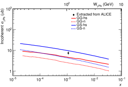
The LHC experiments have only measured the integrated cross sections, as the experimental methods are based on template fits. For the incoherent photoproduction, there exists only one datapoint from ALICE at at midrapidity Abbas:2013oua . At midrapidity there is no ambiquity in determining the Bjorken-, and the photoproduction cross section at can be extracted as the photon flux is known. In Fig. 11 the predicted incoherent photoproduction cross section as a function of is shown, based on Ref. Cepila:2017nef . The predictions from the calculations that both include and do not include nucleon substructure fluctuations (where the number of hot spots depends on , see Eq. (17)) are shown. The substructure is shown to enhance the incoherent cross section almost by a factor of , which is consistent with the ALICE data. It is important to note that the predicted absolute normalization depends strongly on the applied wave function, and simultaneous comparison to both coherent and incoherent data is necessary. Cross section ratios are theoretically more robust. In Ref. Mantysaari:2017dwh it was shown that the wave function uncertainty almost cancels in the incoherent-to-coherent ratio, and the nucleon substructure fluctuations improve the description of the ALICE data, which still has a quite large uncertainty (see also Ref. Sambasivam:2019gdd ).
VI.2 Nucleon substructure and flow in heavy ion collisions
Collective phenomena are traditionally seen as a proof of the formation of the Quark Gluon Plasma (QGP) in heavy ion collisions at high energy. However, recently similar signals have been also observed in high multiplicity proton-proton and proton-nucleus collisions. This suggests that a hydrodynamically evolving medium may be produced also in smaller collision systems. As the proton shape fluctuations result in initial state anisotropies Welsh:2016siu , the event-by-event fluctuating proton structure can in principle be constrained by comparing hydrodynamical simulations including proton shape fluctuations with experimental data. However, there are additional sources of momentum correlations that do not require a medium formation and could contribute significantly to the measured collective effects. Also, not all effects traditionally associated with the QGP production are seen in small system collisions. For example, production of high transverse momentum particles is suppressed in heavy ion collisions, and this effect is understood to be caused by partons losing energy when propagating through the medium. Similar effects are not seen in even the highest multiplicity proton-proton and proton-nucleus collisions. For a review, the reader is referred to Ref. Dusling:2015gta .
Theoretically it is also not a priori clear if a locally thermalised fluid can be produced in such a small systems. The applicability of hydrodynamics can also be limited by the presence of large density gradients Niemi:2014wta , at least if the multiplicities are not very high. The highest multiplicity events, on the other hand, may only be produced by a subset of rare proton configurations Coleman-Smith:2013rla .
In Sec. IV.1 it was shown how the Wilson lines, encoding all the information about the small- structure, can be constrained based on diffractive vector meson production data. This can be taken as an input for hydrodynamical simulations of the proton-nucleus (and in principle proton-proton) collisions e.g. in the framework developed in Ref. Schenke:2012wb . There, the developed IP-Glasma model is first used to determine the initial state after the collision, and to solve the early time evolution (see also Refs. Giacalone:2019kgg ; Giacalone:2019vwh for a recent develompent of the fluctuating initial condition for the hydrodynamical evolution from the CGC framework). When the system is close to the local thermal equilibrium, hydrodynamical evolution is applied using the relativistic viscous hydrodynamic simulation MUSIC Schenke:2010nt ; Schenke:2010rr . After the hydrodynamical phase the final final stages of the evolution for the produced particles are simulated by using the UrQMD model which implements the microscopic Boltzmann equation Bass:1998ca ; Bleicher:1999xi .
In general, as the hydrodynamical evolution translates spatial anisotropies into the momentum space correlations, if the colliding proton is spherical, only small momentum space anisotropies can be expected. In the IP-Glasma+hydrodynamics framework this expectation was confirmed in Ref. Schenke:2014zha . When the proton shape fluctuations determined in Sec. IV.1 were used, a good description of the measured elliptic and triangular flow coefficient and defined in Eq. (21) in high-multiplicity proton-lead collisions were obtained Mantysaari:2017cni . Similarly, in Ref. Weller:2017tsr it was found that a three valence quark structure for the nucleons is necessary in hydrodynamical simulations of proton-proton, proton-lead and lead-lead collisions. For the effect of proton substructure on the initial state structure (e.g. eccentricities), see Ref. Welsh:2016siu .
Another approach to determine the proton shape fluctuations is to first consider hydrodynamical simulations of lead-lead and proton-lead collisions with different nucleon shape fluctuations, and by comparing with experimental measurements to deduce the preferred shape fluctuations. A major complication in this approach is that the hydrodynamical simulations are computationally intensive, and it is in practice not possible to produce enough statistics with different descriptions of the fluctuating initial state to perform a straightforward minimization procedure.
A powerful approach that can be used to determine the initial state is based on Bayesian statistics. In the context of heavy ion collisions, this approach has been used recently to constrain the fundamental properties of the produced Quark Gluon Plasma (QGP). These properties include, for example, the temperature dependence of the shear and bulk viscosities and the temperature at which the hydrodynamical evolution ends and the medium is converted into particles whose subsequent evolution is also included by using the UrQMD model. The method developed in Ref. Bernhard:2016tnd (see recent highlights in Ref. Bernhard:2019bmu ) uses a Gaussian process emulator that is trained to effectively interpolate in the multi dimensional parameter space. Applying Bayesian statistics and numerically light emulator techniques, it becomes possible to construct the likelihood distributions for the model parameters. As a result, fundamental properties of the QGP with uncertainty estimates are obtained.
To determine the proton shape fluctuations based on high-multiplicity proton-nucleus data from RHIC and from the LHC, this approach was generalized in Ref. Moreland:2018gsh to include a hot spot structure for the nucleons. The number of hot spots, as well as their size, are model parameters along with the QGP properties mentioned above. Important observables sensitive to the hot spot structure that are used to calibrate the Gaussian emulator are e.g. mean transverse momenta and flow cumulant measurements made in proton-lead collisions. Also, data from lead-lead collisions is included in the analysis.
From the obtained posterior distributions, it is possible to sample the most likely parametrizations describing the nucleon structure fluctuations, as well as QGP properties and the correlations between the different parameters. In Fig. 12 the centrality dependence of the elliptic () and triangular () flow coefficients are calculated from 100 random parametrizations sampled from the posterior distribution, and compared with the CMS data Chatrchyan:2013nka (also used to train the emulator). A reasonable description of the flow harmonics, as well as of the centrality dependence of the charge particle yield, are obtained. Simultaneously, e.g. the flow harmonics measured in lead-lead collisions are described accurately and with a much smaller variation between the different parametrizations sampled from the posterior distribution than in the case of proton-lead collisions.
For the nucleon, the analysis in Ref. Moreland:2018gsh prefers many hot spots (). For the hot spot size, and for the size of the nucleon, the posterior distribution is illustrated in Fig. 13. When comparing these results with the proton shapes constrained by diffractive production data and succesfully used to describe proton-lead collisions in the IP-Glasmahydrodynamics framework, one notices that the obtained protons and hot spot sizes seem to be much larger. However, the density profiles can not be directly compared. The analysis of Ref. Moreland:2018gsh prefers the entropy production to be proportional to the geometric mean of the density profiles of the two nuclei. Thus, in proton-nucleus collisions the initial entropy deposition scales as , where and are the transverse density profiles for the nucleus and for the proton, respectively. On the other hand, in the IP-Glasma framework the initial entropy deposition scales as .
In central (high multiplicity) collisions the nuclear density is approximatively constant and dependence on is weak. Consequently, one should compare the squared proton density profile from Ref. Moreland:2018gsh to the IP-Glasma density profile. For example, the Gaussian width for the hot spot size obtained in Ref. Moreland:2018gsh is (when the hot spot profile is ). The squared density profile then corresponds to a Gaussian distribution that has a width parameter . This should be compared to the hot spot width obtained by fitting the data as discussed in Sec. IV.1. Although the parametrizations are still not exactly compatible, qualitatively they suggest a similar fluctuating substructure for the proton. On the other hand, the differences demonstrate the limitations of the current approaches to quantitatively extract the fluctuating nucleon shapes from hadronic collisions, as the results depend on the details of the particle production mechanism.


VII Outlook
Multiple measurements from different collider experiments suggest that there are significant quantum mechanical event-by-event fluctuations in the transverse profile of the proton at small Bjorken-. This picture is obtained by analysing elastic and diffractive scattering processes, as well as correlations observed in high multiplicity proton-proton and proton-lead collisions.
Even though the qualitative picture pointing towards sizeable event-by-event fluctuations is the same based on all these observables, different processes that probe the proton structure at different scales result in e.g. different sizes for the hot spots. At this point it is not clear how, for example, results from elastic low momentum transfer proton-proton collisions can be related to the proton shape fluctuations extracted by studying exclusive production of heavy vector mesons which is a perturbative process. Similarly, in analyses of collective phenomena in high multiplicity collisions one is actually sensitive to the initial energy density or entropy production before the hydrodynamical evolution, which may differ from the transverse shape of the proton.
In heavy nuclei, the proton and neutron shape fluctuations are usually suppressed, and the fluctuating nucleonic structure dominates many observables that are sensitive to the initial state fluctuations. However, there are processes such as exclusive vector meson production at high momentum transfer that probe fluctuations at small distance scales and as such, can be used to determine if the fluctuating structure of protons and neutrons is modified in the nuclear environment.
In the near future, large amounts of new data is expected to help constraining proton shape fluctuations in more detail. Detailed correlation measurements form high multiplicity proton-proton and proton-nucleus collisions at the LHC, as well as proton-light ion or light-heavy-ion collisions at RHIC will provide useful data. Photoproduction studies in ultra peripheral collisions at the LHC, and DIS experiments in a next generation Electron Ion Collider in the US Boer:2011fh ; Accardi:2012qut ; Aschenauer:2017jsk , Europe AbelleiraFernandez:2012cc or China Chen:2018wyz will provide vast amounts of precise data probing the structure of protons and nuclei with high precision.
On the theory side, developments need to stay in pace with the experimental advances. Existing Monte Carlo event generators, such as Sarre Toll:2012mb ; Toll:2013gda which simulates exclusive vector meson production at the EIC, could be updated to include nucleon shape fluctuations. More generally, there are two important paths for theory developments. First, perturbative calculations need to be developed to next-to-leading order accuracy in the QCD coupling to achieve precision level (see e.g. Refs. Balitsky:2008zza ; Balitsky:2010ze ; Balitsky:2013fea ; Kovner:2013ona ; Lappi:2015fma ; Lappi:2016fmu ; Boussarie:2016bkq ; Hanninen:2017ddy ; Ducloue:2017ftk ; Beuf:2017bpd ; Ducloue:2019ezk ; Kang:2019ysm for recent developments in the Color Glass Condensate framework). Additionally, new more differential observables are needed to probe the proton and nuclear structure in more detail. For example, dijet production at high energies is a promising observable in ultraperipheral collisions at the LHC ATLAS:2017kwa and in a future Electron-Ion Collider Dumitru:2018kuw , as the second momentum vector provides an additional handle to the geometry and potentially enables more precise extraction of the proton and nuclear shape fluctuations. It may even be possible to extract properties of the Wigner distribution that describes how partons are distributed both as a function of transverse coordinate and transverse momentum Hatta:2016dxp ; Hagiwara:2017fye ; Salazar:2019ncp ; Mantysaari:2019csc ; Mantysaari:2019hkq . The effect of nucleon substructure fluctuations on multi particle interactions (MPIs) should also be studied, as these processes can potentially provide complementary constraints on the shape fluctuations.
Acknowledgements
This work was supported by the Academy of Finland project 314764. I thank B. Schenke for useful comments and T. Lappi for a careful reading of the manuscript.
References
- (1) H1, ZEUS collaboration, F. D. Aaron et. al., Combined Measurement and QCD Analysis of the Inclusive Scattering Cross Sections at HERA, JHEP 01 (2010) 109 [arXiv:0911.0884 [hep-ex]].
- (2) H1, ZEUS collaboration, H. Abramowicz et. al., Combination of measurements of inclusive deep inelastic scattering cross sections and QCD analysis of HERA data, Eur. Phys. J. C75 (2015) no. 12 580 [arXiv:1506.06042 [hep-ex]].
- (3) D. Müller, D. Robaschik, B. Geyer, F. M. Dittes and J. Hořejši, Wave functions, evolution equations and evolution kernels from light ray operators of QCD, Fortsch. Phys. 42 (1994) 101 [arXiv:hep-ph/9812448 [hep-ph]].
- (4) X.-D. Ji, Deeply virtual Compton scattering, Phys. Rev. D55 (1997) 7114 [arXiv:hep-ph/9609381 [hep-ph]].
- (5) A. V. Radyushkin, Nonforward parton distributions, Phys. Rev. D56 (1997) 5524 [arXiv:hep-ph/9704207 [hep-ph]].
- (6) J. C. Collins, L. Frankfurt and M. Strikman, Factorization for hard exclusive electroproduction of mesons in QCD, Phys. Rev. D56 (1997) 2982 [arXiv:hep-ph/9611433 [hep-ph]].
- (7) M. G. Ryskin, Diffractive J / psi electroproduction in LLA QCD, Z. Phys. C57 (1993) 89.
- (8) M. L. Good and W. D. Walker, Diffraction disssociation of beam particles, Phys. Rev. 120 (1960) 1857.
- (9) H. I. Miettinen and J. Pumplin, Diffraction Scattering and the Parton Structure of Hadrons, Phys. Rev. D18 (1978) 1696.
- (10) H. Kowalski, L. Motyka and G. Watt, Exclusive diffractive processes at HERA within the dipole picture, Phys. Rev. D74 (2006) 074016 [arXiv:hep-ph/0606272 [hep-ph]].
- (11) A. Caldwell and H. Kowalski in Elastic and Diffractive Scattering. Proceedings, 13th International Conference, Blois Workshop, CERN, Geneva, Switzerland, June 29-July 3, 2009, pp. 190–192, 2009. arXiv:0909.1254 [hep-ph].
- (12) L. L. Frankfurt, G. A. Miller and M. Strikman, The Geometrical color optics of coherent high-energy processes, Ann. Rev. Nucl. Part. Sci. 44 (1994) 501 [arXiv:hep-ph/9407274 [hep-ph]].
- (13) M. Diehl, Generalized parton distributions, Phys. Rept. 388 (2003) 41 [arXiv:hep-ph/0307382 [hep-ph]].
- (14) A. Accardi et. al., Electron Ion Collider: The Next QCD Frontier, Eur. Phys. J. A52 (2016) no. 9 268 [arXiv:1212.1701 [nucl-ex]].
- (15) T. Lappi, H. Mäntysaari and R. Venugopalan, Ballistic protons in incoherent exclusive vector meson production as a measure of rare parton fluctuations at an Electron-Ion Collider, Phys. Rev. Lett. 114 (2015) no. 8 082301 [arXiv:1411.0887 [hep-ph]].
- (16) A. H. Mueller, Soft gluons in the infinite momentum wave function and the BFKL pomeron, Nucl. Phys. B415 (1994) 373.
- (17) N. Nikolaev and B. G. Zakharov, Pomeron structure function and diffraction dissociation of virtual photons in perturbative QCD, Z. Phys. C53 (1992) 331.
- (18) Y. V. Kovchegov and E. Levin, Quantum chromodynamics at high energy, Camb. Monogr. Part. Phys. Nucl. Phys. Cosmol. 33 (2012) 1.
- (19) E. Iancu and R. Venugopalan in Quark-gluon plasma 4 (R. C. Hwa and X.-N. Wang, eds.), pp. 249–3363. 2003. arXiv:hep-ph/0303204 [hep-ph].
- (20) F. Gelis, E. Iancu, J. Jalilian-Marian and R. Venugopalan, The Color Glass Condensate, Ann. Rev. Nucl. Part. Sci. 60 (2010) 463 [arXiv:1002.0333 [hep-ph]].
- (21) J. L. Albacete and C. Marquet, Gluon saturation and initial conditions for relativistic heavy ion collisions, Prog. Part. Nucl. Phys. 76 (2014) 1 [arXiv:1401.4866 [hep-ph]].
- (22) J.-P. Blaizot, High gluon densities in heavy ion collisions, Rept. Prog. Phys. 80 (2017) no. 3 032301 [arXiv:1607.04448 [hep-ph]].
- (23) J. Bartels, K. J. Golec-Biernat and K. Peters, On the dipole picture in the nonforward direction, Acta Phys. Polon. B34 (2003) 3051 [arXiv:hep-ph/0301192 [hep-ph]].
- (24) Y. Hatta, B.-W. Xiao and F. Yuan, Gluon Tomography from Deeply Virtual Compton Scattering at Small-x, Phys. Rev. D95 (2017) no. 11 114026 [arXiv:1703.02085 [hep-ph]].
- (25) S. Munier, A. M. Stasto and A. H. Mueller, Impact parameter dependent S matrix for dipole proton scattering from diffractive meson electroproduction, Nucl. Phys. B603 (2001) 427 [arXiv:hep-ph/0102291 [hep-ph]].
- (26) J. P. Ralston and B. Pire, Femtophotography of protons to nuclei with deeply virtual Compton scattering, Phys. Rev. D66 (2002) 111501 [arXiv:hep-ph/0110075 [hep-ph]].
- (27) U. Amaldi and K. R. Schubert, Impact Parameter Interpretation of Proton Proton Scattering from a Critical Review of All ISR Data, Nucl. Phys. B166 (1980) 301.
- (28) A. G. Shuvaev, K. J. Golec-Biernat, A. D. Martin and M. G. Ryskin, Off diagonal distributions fixed by diagonal partons at small x and xi, Phys. Rev. D60 (1999) 014015 [arXiv:hep-ph/9902410 [hep-ph]].
- (29) H. Mäntysaari and B. Schenke, Probing subnucleon scale fluctuations in ultraperipheral heavy ion collisions, Phys. Lett. B772 (2017) 832 [arXiv:1703.09256 [hep-ph]].
- (30) V. Guzey and M. Zhalov, Exclusive production in ultraperipheral collisions at the LHC: constrains on the gluon distributions in the proton and nuclei, JHEP 10 (2013) 207 [arXiv:1307.4526 [hep-ph]].
- (31) L. Zheng, E. C. Aschenauer and J. H. Lee, Determination of electron-nucleus collision geometry with forward neutrons, Eur. Phys. J. A50 (2014) no. 12 189 [arXiv:1407.8055 [hep-ex]].
- (32) J. Jalilian-Marian, A. Kovner, L. D. McLerran and H. Weigert, The Intrinsic glue distribution at very small x, Phys. Rev. D55 (1997) 5414 [arXiv:hep-ph/9606337 [hep-ph]].
- (33) J. Jalilian-Marian, A. Kovner, A. Leonidov and H. Weigert, The BFKL equation from the Wilson renormalization group, Nucl. Phys. B504 (1997) 415 [arXiv:hep-ph/9701284 [hep-ph]].
- (34) J. Jalilian-Marian, A. Kovner, A. Leonidov and H. Weigert, The Wilson renormalization group for low x physics: Towards the high density regime, Phys. Rev. D59 (1998) 014014 [arXiv:hep-ph/9706377 [hep-ph]].
- (35) E. Iancu and L. D. McLerran, Saturation and universality in QCD at small x, Phys. Lett. B510 (2001) 145 [arXiv:hep-ph/0103032 [hep-ph]].
- (36) I. Balitsky and G. A. Chirilli, Rapidity evolution of Wilson lines at the next-to-leading order, Phys. Rev. D88 (2013) 111501 [arXiv:1309.7644 [hep-ph]].
- (37) A. Kovner, M. Lublinsky and Y. Mulian, Jalilian-Marian, Iancu, McLerran, Weigert, Leonidov, Kovner evolution at next to leading order, Phys. Rev. D89 (2014) no. 6 061704 [arXiv:1310.0378 [hep-ph]].
- (38) Y. V. Kovchegov, Small x F(2) structure function of a nucleus including multiple pomeron exchanges, Phys. Rev. D60 (1999) 034008 [arXiv:hep-ph/9901281 [hep-ph]].
- (39) I. Balitsky, Operator expansion for high-energy scattering, Nucl. Phys. B463 (1996) 99 [arXiv:hep-ph/9509348 [hep-ph]].
- (40) I. Balitsky and G. A. Chirilli, Next-to-leading order evolution of color dipoles, Phys. Rev. D77 (2008) 014019 [arXiv:0710.4330 [hep-ph]].
- (41) J. L. Albacete, N. Armesto, J. G. Milhano, P. Quiroga-Arias and C. A. Salgado, AAMQS: A non-linear QCD analysis of new HERA data at small-x including heavy quarks, Eur. Phys. J. C71 (2011) 1705 [arXiv:1012.4408 [hep-ph]].
- (42) T. Lappi and H. Mäntysaari, Single inclusive particle production at high energy from HERA data to proton-nucleus collisions, Phys. Rev. D88 (2013) 114020 [arXiv:1309.6963 [hep-ph]].
- (43) B. Ducloué, E. Iancu, G. Soyez and D. N. Triantafyllopoulos, HERA data and collinearly-improved BK dynamics, Phys. Lett. B803 (2020) 135305 [arXiv:1912.09196 [hep-ph]].
- (44) J. Berger and A. M. Stasto, Small x nonlinear evolution with impact parameter and the structure function data, Phys. Rev. D84 (2011) 094022 [arXiv:1106.5740 [hep-ph]].
- (45) H. Mäntysaari and B. Schenke, Confronting impact parameter dependent JIMWLK evolution with HERA data, Phys. Rev. D98 (2018) no. 3 034013 [arXiv:1806.06783 [hep-ph]].
- (46) H. Kowalski and D. Teaney, An Impact parameter dipole saturation model, Phys. Rev. D68 (2003) 114005 [arXiv:hep-ph/0304189 [hep-ph]].
- (47) A. H. Rezaeian, M. Siddikov, M. Van de Klundert and R. Venugopalan, Analysis of combined HERA data in the Impact-Parameter dependent Saturation model, Phys. Rev. D87 (2013) no. 3 034002 [arXiv:1212.2974 [hep-ph]].
- (48) H. Mäntysaari and P. Zurita, In depth analysis of the combined HERA data in the dipole models with and without saturation, Phys. Rev. D98 (2018) 036002 [arXiv:1804.05311 [hep-ph]].
- (49) V. N. Gribov and L. N. Lipatov, Deep inelastic e p scattering in perturbation theory, Sov. J. Nucl. Phys. 15 (1972) 438. [Yad. Fiz.15,781(1972)].
- (50) V. N. Gribov and L. N. Lipatov, e+ e- pair annihilation and deep inelastic e p scattering in perturbation theory, Sov. J. Nucl. Phys. 15 (1972) 675. [Yad. Fiz.15,1218(1972)].
- (51) G. Altarelli and G. Parisi, Asymptotic Freedom in Parton Language, Nucl. Phys. B126 (1977) 298.
- (52) Y. L. Dokshitzer, Calculation of the Structure Functions for Deep Inelastic Scattering and e+ e- Annihilation by Perturbation Theory in Quantum Chromodynamics., Sov. Phys. JETP 46 (1977) 641. [Zh. Eksp. Teor. Fiz.73,1216(1977)].
- (53) S. Anand and T. Toll, Exclusive diffractive vector meson production: A comparison between the dipole model and the leading twist shadowing approach, Phys. Rev. C100 (2019) no. 2 024901 [arXiv:1807.10888 [hep-ph]].
- (54) ZEUS collaboration, J. Breitweg et. al., Measurement of diffractive photoproduction of vector mesons at large momentum transfer at HERA, Eur. Phys. J. C14 (2000) 213 [arXiv:hep-ex/9910038 [hep-ex]].
- (55) ZEUS collaboration, S. Chekanov et. al., Exclusive photoproduction of J / psi mesons at HERA, Eur. Phys. J. C24 (2002) 345 [arXiv:hep-ex/0201043 [hep-ex]].
- (56) H1 collaboration, A. Aktas et. al., Diffractive photoproduction of mesons with large momentum transfer at HERA, Phys. Lett. B568 (2003) 205 [arXiv:hep-ex/0306013 [hep-ex]].
- (57) ZEUS collaboration, S. Chekanov et. al., Exclusive electroproduction of J/psi mesons at HERA, Nucl. Phys. B695 (2004) 3 [arXiv:hep-ex/0404008 [hep-ex]].
- (58) H1 collaboration, A. Aktas et. al., Elastic J/psi production at HERA, Eur. Phys. J. C46 (2006) 585 [arXiv:hep-ex/0510016 [hep-ex]].
- (59) ZEUS collaboration, S. Chekanov et. al., Measurement of J/psi photoproduction at large momentum transfer at HERA, JHEP 05 (2010) 085 [arXiv:0910.1235 [hep-ex]].
- (60) H1 collaboration, C. Alexa et. al., Elastic and Proton-Dissociative Photoproduction of J/psi Mesons at HERA, Eur. Phys. J. C73 (2013) no. 6 2466 [arXiv:1304.5162 [hep-ex]].
- (61) H1 collaboration, C. Adloff et. al., Elastic electroproduction of rho mesons at HERA, Eur. Phys. J. C13 (2000) 371 [arXiv:hep-ex/9902019 [hep-ex]].
- (62) H1 collaboration, S. Aid et. al., Elastic electroproduction of and mesons at large Q2 at HERA, Nucl. Phys. B468 (1996) 3 [arXiv:hep-ex/9602007 [hep-ex]]. [Erratum: Nucl. Phys.B548,639(1999)].
- (63) ZEUS collaboration, S. Chekanov et. al., Exclusive rho0 production in deep inelastic scattering at HERA, PMC Phys. A1 (2007) 6 [arXiv:0708.1478 [hep-ex]].
- (64) H1 collaboration, F. D. Aaron et. al., Diffractive Electroproduction of rho and phi Mesons at HERA, JHEP 05 (2010) 032 [arXiv:0910.5831 [hep-ex]].
- (65) ZEUS collaboration, S. Chekanov et. al., Exclusive electroproduction of phi mesons at HERA, Nucl. Phys. B718 (2005) 3 [arXiv:hep-ex/0504010 [hep-ex]].
- (66) ZEUS collaboration, J. Breitweg et. al., Measurement of elastic Upsilon photoproduction at HERA, Phys. Lett. B437 (1998) 432 [arXiv:hep-ex/9807020 [hep-ex]].
- (67) ZEUS collaboration, S. Chekanov et. al., Exclusive photoproduction of upsilon mesons at HERA, Phys. Lett. B680 (2009) 4 [arXiv:0903.4205 [hep-ex]].
- (68) H1 collaboration, C. Adloff et. al., Elastic photoproduction of J / psi and Upsilon mesons at HERA, Phys. Lett. B483 (2000) 23 [arXiv:hep-ex/0003020 [hep-ex]].
- (69) H. Mäntysaari and B. Schenke, Evidence of strong proton shape fluctuations from incoherent diffraction, Phys. Rev. Lett. 117 (2016) no. 5 052301 [arXiv:1603.04349 [hep-ph]].
- (70) N. Armesto and A. H. Rezaeian, Exclusive vector meson production at high energies and gluon saturation, Phys. Rev. D90 (2014) no. 5 054003 [arXiv:1402.4831 [hep-ph]].
- (71) J. T. Mitchell, D. V. Perepelitsa, M. J. Tannenbaum and P. W. Stankus, Tests of constituent-quark generation methods which maintain both the nucleon center of mass and the desired radial distribution in Monte Carlo Glauber models, Phys. Rev. C93 (2016) no. 5 054910 [arXiv:1603.08836 [nucl-ex]].
- (72) H. Mäntysaari and B. Schenke, Revealing proton shape fluctuations with incoherent diffraction at high energy, Phys. Rev. D94 (2016) no. 3 034042 [arXiv:1607.01711 [hep-ph]].
- (73) J. Cepila, J. G. Contreras and J. D. Tapia Takaki, Energy dependence of dissociative photoproduction as a signature of gluon saturation at the LHC, Phys. Lett. B766 (2017) 186 [arXiv:1608.07559 [hep-ph]].
- (74) T. Lappi and H. Mantysaari, Incoherent diffractive J-production in high energy nuclear DIS, Phys. Rev. C83 (2011) 065202 [arXiv:1011.1988 [hep-ph]].
- (75) L. McLerran and P. Tribedy, Intrinsic Fluctuations of the Proton Saturation Momentum Scale in High Multiplicity p+p Collisions, Nucl. Phys. A945 (2016) 216 [arXiv:1508.03292 [hep-ph]].
- (76) F. Bissey, F.-G. Cao, A. R. Kitson, A. I. Signal, D. B. Leinweber, B. G. Lasscock and A. G. Williams, Gluon flux-tube distribution and linear confinement in baryons, Phys. Rev. D76 (2007) 114512 [arXiv:hep-lat/0606016 [hep-lat]].
- (77) L. D. McLerran and R. Venugopalan, Computing quark and gluon distribution functions for very large nuclei, Phys. Rev. D49 (1994) 2233 [arXiv:hep-ph/9309289 [hep-ph]].
- (78) F. Dominguez, C. Marquet and B. Wu, On multiple scatterings of mesons in hot and cold QCD matter, Nucl. Phys. A823 (2009) 99 [arXiv:0812.3878 [nucl-th]].
- (79) C. Marquet and B. Wu in Proceedings, 17th International Workshop on Deep-Inelastic Scattering and Related Subjects (DIS 2009): Madrid, Spain, April 26-30, 2009, p. 176, 2009. arXiv:0908.4180 [hep-ph].
- (80) M. C. Traini and J.-P. Blaizot, Diffractive incoherent vector meson production off protons: a quark model approach to gluon fluctuation effects, Eur. Phys. J. C79 (2019) no. 4 327 [arXiv:1804.06110 [hep-ph]].
- (81) ALICE collaboration, B. B. Abelev et. al., Exclusive photoproduction off protons in ultra-peripheral p-Pb collisions at TeV, Phys. Rev. Lett. 113 (2014) no. 23 232504 [arXiv:1406.7819 [nucl-ex]].
- (82) ALICE collaboration, S. Acharya et. al., Energy dependence of exclusive photoproduction off protons in ultra-peripheral p–Pb collisions at TeV, Eur. Phys. J. C79 (2019) no. 5 402 [arXiv:1809.03235 [nucl-ex]].
- (83) C. A. Bertulani, S. R. Klein and J. Nystrand, Physics of ultra-peripheral nuclear collisions, Ann. Rev. Nucl. Part. Sci. 55 (2005) 271 [arXiv:nucl-ex/0502005 [nucl-ex]].
- (84) S. R. Klein and H. Mäntysaari, Imaging the nucleus with high-energy photons, Nature Rev. Phys. 1 (2019) no. 11 662 [arXiv:1910.10858 [hep-ex]].
- (85) J. Cepila, J. G. Contreras and M. Krelina, Coherent and incoherent photonuclear production in an energy-dependent hot-spot model, Phys. Rev. C97 (2018) no. 2 024901 [arXiv:1711.01855 [hep-ph]].
- (86) J. Cepila, J. G. Contreras, M. Krelina and J. D. Tapia Takaki, Mass dependence of vector meson photoproduction off protons and nuclei within the energy-dependent hot-spot model, Nucl. Phys. B934 (2018) 330 [arXiv:1804.05508 [hep-ph]].
- (87) T. Liou, A. H. Mueller and S. Munier, Fluctuations of the multiplicity of produced particles in onium-nucleus collisions, Phys. Rev. D95 (2017) no. 1 014001 [arXiv:1608.00852 [hep-ph]].
- (88) L. Dominé, G. Giacalone, C. Lorcé, S. Munier and S. Pekar, Gluon density fluctuations in dilute hadrons, Phys. Rev. D98 (2018) no. 11 114032 [arXiv:1810.05049 [hep-ph]].
- (89) J. L. Albacete and A. Soto-Ontoso, Hot spots and the hollowness of proton–proton interactions at high energies, Phys. Lett. B770 (2017) 149 [arXiv:1605.09176 [hep-ph]].
- (90) TOTEM collaboration, G. Antchev et. al., Proton-proton elastic scattering at the LHC energy of s** (1/2) = 7-TeV, EPL 95 (2011) no. 4 41001 [arXiv:1110.1385 [hep-ex]].
- (91) TOTEM collaboration, G. Antchev et. al., Elastic differential cross-section at and implications on the existence of a colourless C-odd three-gluon compound state, Eur. Phys. J. C80 (2020) no. 2 91 [arXiv:1812.08610 [hep-ex]].
- (92) TOTEM collaboration, G. Antchev et. al., Elastic differential cross-section measurement at TeV by TOTEM, Eur. Phys. J. C79 (2019) no. 10 861 [arXiv:1812.08283 [hep-ex]].
- (93) COMPETE collaboration, J. R. Cudell, V. V. Ezhela, P. Gauron, K. Kang, Yu. V. Kuyanov, S. B. Lugovsky, E. Martynov, B. Nicolescu, E. A. Razuvaev and N. P. Tkachenko, Benchmarks for the forward observables at RHIC, the Tevatron Run II and the LHC, Phys. Rev. Lett. 89 (2002) 201801 [arXiv:hep-ph/0206172 [hep-ph]].
- (94) TOTEM collaboration, G. Antchev et. al., First determination of the parameter at TeV: probing the existence of a colourless C-odd three-gluon compound state, Eur. Phys. J. C79 (2019) no. 9 785 [arXiv:1812.04732 [hep-ex]].
- (95) A. Alkin, E. Martynov, O. Kovalenko and S. M. Troshin, Impact-parameter analysis of TOTEM data at the LHC: Black disk limit exceeded, Phys. Rev. D89 (2014) no. 9 091501 [arXiv:1403.8036 [hep-ph]].
- (96) I. M. Dremin, Will protons become gray at 13 TeV and 100 TeV?, Bull. Lebedev Phys. Inst. 44 (2017) no. 4 94 [arXiv:1511.03212 [hep-ph]].
- (97) S. M. Troshin and N. E. Tyurin, The new scattering mode emerging at the LHC?, Mod. Phys. Lett. A31 (2016) no. 13 1650079 [arXiv:1602.08972 [hep-ph]].
- (98) E. Ruiz Arriola and W. Broniowski, Proton–Proton On Shell Optical Potential at High Energies and the Hollowness Effect, Few Body Syst. 57 (2016) no. 7 485 [arXiv:1602.00288 [hep-ph]].
- (99) J. L. Albacete, H. Petersen and A. Soto-Ontoso, Symmetric cumulants as a probe of the proton substructure at LHC energies, Phys. Lett. B778 (2018) 128 [arXiv:1707.05592 [hep-ph]].
- (100) H. Niemi, G. S. Denicol, H. Holopainen and P. Huovinen, Event-by-event distributions of azimuthal asymmetries in ultrarelativistic heavy-ion collisions, Phys. Rev. C87 (2013) no. 5 054901 [arXiv:1212.1008 [nucl-th]].
- (101) P. Bozek and W. Broniowski, Collective dynamics in high-energy proton-nucleus collisions, Phys. Rev. C88 (2013) no. 1 014903 [arXiv:1304.3044 [nucl-th]].
- (102) B. Schenke, C. Shen and P. Tribedy, Hybrid Color Glass Condensate and hydrodynamic description of the Relativistic Heavy Ion Collider small system scan, Phys. Lett. B803 (2020) 135322 [arXiv:1908.06212 [nucl-th]].
- (103) CMS collaboration, A. M. Sirunyan et. al., Observation of Correlated Azimuthal Anisotropy Fourier Harmonics in and Collisions at the LHC, Phys. Rev. Lett. 120 (2018) no. 9 092301 [arXiv:1709.09189 [nucl-ex]].
- (104) ALICE collaboration, S. Acharya et. al., Investigations of Anisotropic Flow Using Multiparticle Azimuthal Correlations in pp, p-Pb, Xe-Xe, and Pb-Pb Collisions at the LHC, Phys. Rev. Lett. 123 (2019) no. 14 142301 [arXiv:1903.01790 [nucl-ex]].
- (105) J. L. Albacete, H. Niemi, H. Petersen and A. Soto-Ontoso, Correlated gluonic hot spots meet symmetric cumulants data at LHC energies, Nucl. Phys. A982 (2019) 463 [arXiv:1807.05866 [hep-ph]].
- (106) H. Mäntysaari and B. Schenke, Accessing the gluonic structure of light nuclei at a future electron-ion collider, Phys. Rev. C101 (2020) no. 1 015203 [arXiv:1910.03297 [hep-ph]].
- (107) T. Toll and T. Ullrich, Exclusive diffractive processes in electron-ion collisions, Phys. Rev. C87 (2013) no. 2 024913 [arXiv:1211.3048 [hep-ph]].
- (108) T. Lappi and H. Mantysaari, production in ultraperipheral Pb+Pb and +Pb collisions at energies available at the CERN Large Hadron Collider, Phys. Rev. C87 (2013) no. 3 032201 [arXiv:1301.4095 [hep-ph]].
- (109) ALICE collaboration, E. Abbas et. al., Charmonium and pair photoproduction at mid-rapidity in ultra-peripheral Pb-Pb collisions at =2.76 TeV, Eur. Phys. J. C73 (2013) no. 11 2617 [arXiv:1305.1467 [nucl-ex]].
- (110) B. Sambasivam, T. Toll and T. Ullrich, Investigating saturation effects in ultraperipheral collisions at the LHC with the color dipole model, Phys. Lett. B803 (2020) 135277 [arXiv:1910.02899 [hep-ph]].
- (111) K. Welsh, J. Singer and U. W. Heinz, Initial state fluctuations in collisions between light and heavy ions, Phys. Rev. C94 (2016) no. 2 024919 [arXiv:1605.09418 [nucl-th]].
- (112) K. Dusling, W. Li and B. Schenke, Novel collective phenomena in high-energy proton–proton and proton–nucleus collisions, Int. J. Mod. Phys. E25 (2016) no. 01 1630002 [arXiv:1509.07939 [nucl-ex]].
- (113) H. Niemi and G. S. Denicol, How large is the Knudsen number reached in fluid dynamical simulations of ultrarelativistic heavy ion collisions?, arXiv:1404.7327 [nucl-th].
- (114) C. E. Coleman-Smith and B. Müller, Mapping the proton’s fluctuating size and shape, Phys. Rev. D89 (2014) 025019 [arXiv:1307.5911 [hep-ph]].
- (115) B. Schenke, P. Tribedy and R. Venugopalan, Fluctuating Glasma initial conditions and flow in heavy ion collisions, Phys. Rev. Lett. 108 (2012) 252301 [arXiv:1202.6646 [nucl-th]].
- (116) G. Giacalone, P. Guerrero-Rodríguez, M. Luzum, C. Marquet and J.-Y. Ollitrault, Fluctuations in heavy-ion collisions generated by QCD interactions in the color glass condensate effective theory, Phys. Rev. C100 (2019) no. 2 024905 [arXiv:1902.07168 [nucl-th]].
- (117) G. Giacalone, F. Gelis, P. Guerrero-Rodríguez, M. Luzum, C. Marquet and J.-Y. Ollitrault, Evolution of fluctuations in the initial state of heavy-ion collisions from RHIC to LHC, arXiv:1911.04720 [nucl-th].
- (118) B. Schenke, S. Jeon and C. Gale, (3+1)D hydrodynamic simulation of relativistic heavy-ion collisions, Phys. Rev. C82 (2010) 014903 [arXiv:1004.1408 [hep-ph]].
- (119) B. Schenke, S. Jeon and C. Gale, Elliptic and triangular flow in event-by-event (3+1)D viscous hydrodynamics, Phys. Rev. Lett. 106 (2011) 042301 [arXiv:1009.3244 [hep-ph]].
- (120) S. A. Bass et. al., Microscopic models for ultrarelativistic heavy ion collisions, Prog. Part. Nucl. Phys. 41 (1998) 255 [arXiv:nucl-th/9803035 [nucl-th]]. [Prog. Part. Nucl. Phys.41,225(1998)].
- (121) M. Bleicher et. al., Relativistic hadron hadron collisions in the ultrarelativistic quantum molecular dynamics model, J. Phys. G25 (1999) 1859 [arXiv:hep-ph/9909407 [hep-ph]].
- (122) B. Schenke and R. Venugopalan, Eccentric protons? Sensitivity of flow to system size and shape in p+p, p+Pb and Pb+Pb collisions, Phys. Rev. Lett. 113 (2014) 102301 [arXiv:1405.3605 [nucl-th]].
- (123) H. Mäntysaari, B. Schenke, C. Shen and P. Tribedy, Imprints of fluctuating proton shapes on flow in proton-lead collisions at the LHC, Phys. Lett. B772 (2017) 681 [arXiv:1705.03177 [nucl-th]].
- (124) R. D. Weller and P. Romatschke, One fluid to rule them all: viscous hydrodynamic description of event-by-event central p+p, p+Pb and Pb+Pb collisions at TeV, Phys. Lett. B774 (2017) 351 [arXiv:1701.07145 [nucl-th]].
- (125) J. E. Bernhard, J. S. Moreland, S. A. Bass, J. Liu and U. Heinz, Applying Bayesian parameter estimation to relativistic heavy-ion collisions: simultaneous characterization of the initial state and quark-gluon plasma medium, Phys. Rev. C94 (2016) no. 2 024907 [arXiv:1605.03954 [nucl-th]].
- (126) J. E. Bernhard, J. S. Moreland and S. A. Bass, Bayesian estimation of the specific shear and bulk viscosity of quark–gluon plasma, Nature Phys. 15 (2019) no. 11 1113.
- (127) J. S. Moreland, J. E. Bernhard and S. A. Bass, Bayesian calibration of a hybrid nuclear collision model using p-Pb and Pb-Pb data at energies available at the CERN Large Hadron Collider, Phys. Rev. C101 (2020) no. 2 024911 [arXiv:1808.02106 [nucl-th]].
- (128) CMS collaboration, S. Chatrchyan et. al., Multiplicity and Transverse Momentum Dependence of Two- and Four-Particle Correlations in pPb and PbPb Collisions, Phys. Lett. B724 (2013) 213 [arXiv:1305.0609 [nucl-ex]].
- (129) D. Boer et. al., Gluons and the quark sea at high energies: Distributions, polarization, tomography, arXiv:1108.1713 [nucl-th].
- (130) E. C. Aschenauer, S. Fazio, J. H. Lee, H. Mantysaari, B. S. Page, B. Schenke, T. Ullrich, R. Venugopalan and P. Zurita, The electron–ion collider: assessing the energy dependence of key measurements, Rept. Prog. Phys. 82 (2019) no. 2 024301 [arXiv:1708.01527 [nucl-ex]].
- (131) LHeC Study Group collaboration, J. L. Abelleira Fernandez et. al., A Large Hadron Electron Collider at CERN: Report on the Physics and Design Concepts for Machine and Detector, J. Phys. G39 (2012) 075001 [arXiv:1206.2913 [physics.acc-ph]].
- (132) X. Chen, A Plan for Electron Ion Collider in China, PoS DIS2018 (2018) 170 [arXiv:1809.00448 [nucl-ex]].
- (133) T. Toll and T. Ullrich, The dipole model Monte Carlo generator Sarre 1, Comput. Phys. Commun. 185 (2014) 1835 [arXiv:1307.8059 [hep-ph]].
- (134) I. Balitsky and G. A. Chirilli, Photon impact factor in the next-to-leading order, Phys. Rev. D83 (2011) 031502 [arXiv:1009.4729 [hep-ph]].
- (135) T. Lappi and H. Mäntysaari, Direct numerical solution of the coordinate space Balitsky-Kovchegov equation at next to leading order, Phys. Rev. D91 (2015) no. 7 074016 [arXiv:1502.02400 [hep-ph]].
- (136) T. Lappi and H. Mäntysaari, Next-to-leading order Balitsky-Kovchegov equation with resummation, Phys. Rev. D93 (2016) no. 9 094004 [arXiv:1601.06598 [hep-ph]].
- (137) R. Boussarie, A. V. Grabovsky, D. Yu. Ivanov, L. Szymanowski and S. Wallon, Next-to-Leading Order Computation of Exclusive Diffractive Light Vector Meson Production in a Saturation Framework, Phys. Rev. Lett. 119 (2017) no. 7 072002 [arXiv:1612.08026 [hep-ph]].
- (138) H. Hänninen, T. Lappi and R. Paatelainen, One-loop corrections to light cone wave functions: the dipole picture DIS cross section, Annals Phys. 393 (2018) 358 [arXiv:1711.08207 [hep-ph]].
- (139) B. Ducloué, H. Hänninen, T. Lappi and Y. Zhu, Deep inelastic scattering in the dipole picture at next-to-leading order, Phys. Rev. D96 (2017) no. 9 094017 [arXiv:1708.07328 [hep-ph]].
- (140) G. Beuf, Dipole factorization for DIS at NLO: Combining the and contributions, Phys. Rev. D96 (2017) no. 7 074033 [arXiv:1708.06557 [hep-ph]].
- (141) B. Ducloué, E. Iancu, A. H. Mueller, G. Soyez and D. N. Triantafyllopoulos, Non-linear evolution in QCD at high-energy beyond leading order, JHEP 04 (2019) 081 [arXiv:1902.06637 [hep-ph]].
- (142) Z.-B. Kang and X. Liu, Power Counting the Small- Observables, arXiv:1910.10166 [hep-ph].
- (143) ATLAS collaboration, T. A. collaboration, Photo-nuclear dijet production in ultra-peripheral Pb+Pb collisions, .
- (144) A. Dumitru, V. Skokov and T. Ullrich, Measuring the Weizsäcker-Williams distribution of linearly polarized gluons at an electron-ion collider through dijet azimuthal asymmetries, Phys. Rev. C99 (2019) no. 1 015204 [arXiv:1809.02615 [hep-ph]].
- (145) Y. Hatta, B.-W. Xiao and F. Yuan, Probing the Small- x Gluon Tomography in Correlated Hard Diffractive Dijet Production in Deep Inelastic Scattering, Phys. Rev. Lett. 116 (2016) no. 20 202301 [arXiv:1601.01585 [hep-ph]].
- (146) Y. Hagiwara, Y. Hatta, R. Pasechnik, M. Tasevsky and O. Teryaev, Accessing the gluon Wigner distribution in ultraperipheral collisions, Phys. Rev. D96 (2017) no. 3 034009 [arXiv:1706.01765 [hep-ph]].
- (147) F. Salazar and B. Schenke, Diffractive dijet production in impact parameter dependent saturation models, Phys. Rev. D100 (2019) no. 3 034007 [arXiv:1905.03763 [hep-ph]].
- (148) H. Mäntysaari, N. Mueller and B. Schenke, Diffractive Dijet Production and Wigner Distributions from the Color Glass Condensate, Phys. Rev. D99 (2019) no. 7 074004 [arXiv:1902.05087 [hep-ph]].
- (149) H. Mäntysaari, N. Mueller, F. Salazar and B. Schenke, Multi-Gluon Correlations and Evidence of Saturation from Dijet Measurements at an Electron Ion Collider, Phys. Rev. Lett. 124 (2020) no. 11 112301 [arXiv:1912.05586 [nucl-th]].