Reverse Diffusion Monte Carlo
Abstract
We propose a Monte Carlo sampler from the reverse diffusion process. Unlike the practice of diffusion models, where the intermediary updates—the score functions—are learned with a neural network, we transform the score matching problem into a mean estimation one. By estimating the means of the regularized posterior distributions, we derive a novel Monte Carlo sampling algorithm called reverse diffusion Monte Carlo (rdMC), which is distinct from the Markov chain Monte Carlo (MCMC) methods. We determine the sample size from the error tolerance and the properties of the posterior distribution to yield an algorithm that can approximately sample the target distribution with any desired accuracy. Additionally, we demonstrate and prove under suitable conditions that sampling with rdMC can be significantly faster than that with MCMC. For multi-modal target distributions such as those in Gaussian mixture models, rdMC greatly improves over the Langevin-style MCMC sampling methods both theoretically and in practice. The proposed rdMC method offers a new perspective and solution beyond classical MCMC algorithms for the challenging complex distributions.
1 Introduction
Recent success of diffusion models has shown great promise for the the reverse diffusion processes in generating samples from a complex distribution (Song et al., 2020; Rombach et al., 2022). In the existing line of works, one is given samples from the target distribution and aims to generate more samples from the same target. One would diffuse the target distribution into a standard normal one, and use score matching to learn the transitions between the consecutive intermediary distributions (Ho et al., 2020; Song et al., 2020). Reversing the learned diffusion process leads us back to the target distribution. The benefit of the reverse diffusion process lies in the efficiency of convergence from any complex distribution to a normal one (Chen et al., 2022a; Lee et al., 2023). For example, diffusing a target multi-modal distribution into a normal one is not harder than diffusing a single mode. Backtracking the process from the normal distribution directly yields the desired multi-modal target. If one instead adopts the forward diffusion process from a normal distribution to the multi-modal one, there is the classical challenge of mixing among the modes, as illustrated in Figure 1. This observation motivates us to ask:
Can we create an efficient, general purpose Monte Carlo sampler from reverse diffusion processes?
For Monte Carlo sampling, while we have access to an unnormalized density function , samples from the target distribution are unavailable (Neal, 1993; Jerrum & Sinclair, 1996; Robert et al., 1999). As a result, we need a different and yet efficient method of score estimation to perform the reverse SDE. This leads to the first contribution of this paper. We leverage the fact that the diffusion process from our target distribution towards a standard normal one is an Ornstein-Uhlenbeck (OU) process, which admits explicit solutions. We thereby transform the score matching problem into a non-parametric mean estimation one, without training a parameterized diffusion model. We name this new algorithm as reverse diffusion Monte Carlo (rdMC).
To implement rdMC and solve the aforementioned mean estimation problem, we propose two approaches. One is to sample from a normal distribution —determined at each time by the transition kernel of the OU process—then compute the mean estimates weighted by the target . This approach translates all the computational challenge to the sample complexity in the importance sampling estimator. The iteration complexity required to achieve an overall TV accuracy is , under minimal assumptions. Another approach is to use Unadjusted Langevin Algorithm (ULA) to generate samples from the product distribution of the target density and the normal one . This approach greatly reduces sample complexity in high dimensions, and yet is a better conditioned algorithm than ULA over due to the multiplication of the normal distribution. In our experiments, we find that a combination of the two approaches excels at distributions with multiple modes.
We then analyze the efficacy and efficiency of our rdMC method. We study the benefits of the reverse diffusion approach for both multi-modal distributions and high dimensional heavy-tail distributions that breaks the isoperimetric properties (Gross, 1975; Poincaré, 1890; Vempala & Wibisono, 2019). In multi-modal distributions, the Langevin algorithm based MCMC approaches suffer from an exponential cost for the need of barrier crossing, which makes mixing time extremely long. The rdMC approach can circumvent the hurdle and solve the problem. For high-dimensional heavy-tail distributions, our rdMC method circumvents the often-required isoperimetric properties of the target distributions, thereby avoiding the curse of dimensionality.
 |
 |
 |
 |
 |
 |
 |
 |
 |
 |
Contributions. We propose a non-parametric sampling algorithm that leverages the reverse SDE of the OU process. Our proposed approach involves estimating the score function by a mean estimation sub-problem for posteriors, enabling the efficient generation of samples through the reverse SDE. We focus on the complexity of the sub-problems and establish the convergence of our algorithm. We found that our approach effectively tackles sampling tasks with ill-conditioned log-Sobolev constants. For example, it excels in challenging scenarios characterized by multi-modal and long-tailed distributions. Our analysis sheds light on the varying complexity of the sub-problems at different time points, providing a fresh perspective for revisiting score estimation in diffusion-based models.
2 Preliminaries
In this section, we begin by introducing related work from the perspectives of Markov Chain Monte Carlo (MCMC) and diffusion models, and we discuss the connection between these works and the present paper. Next, we provide a notation for the reverse process of diffusion models, which specifies the stochastic differential equation (SDE) that particles follow in rdMC.
We first introduce the related works as below.
Langevin-based MCMC. The mainstream gradient-based sampling algorithms are mainly based on the continuous Langevin dynamics (LD) for sampling from a target distribution . The Unadjusted Langevin Algorithm (ULA) discretizes LD using the Euler-Maruyama scheme and obtains a biased stationary distribution. Due to its simplicity, ULA is widely used in machine learning. Its convergence has been investigated for different criteria, including Total Variation (TV) distance, Wasserstein distances (Durmus & Moulines, 2019), and Kullback-Leibler (KL) divergence (Dalalyan, 2017; Cheng & Bartlett, 2018; Ma et al., 2019; Freund et al., 2022), in different settings, such as strongly log-concave, log-Sobolev inequality (LSI) (Vempala & Wibisono, 2019), and Poincaré inequality (PI) (Chewi et al., 2021). Several works have achieved acceleration convergence for ULA by decreasing the discretization error with higher-order SDE, e.g., underdamped Langevin dynamics (Cheng et al., 2018; Ma et al., 2021; Mou et al., 2021), and aligning the discretized stationary distribution to the target , e.g., Metropolis-adjusted Langevin algorithm (Dwivedi et al., 2018) and proximal samplers (Lee et al., 2021b; Chen et al., 2022b; b; Altschuler & Chewi, 2023). Liu & Wang (2016); Dong et al. (2023) also attempt to perform sampling tasks with deterministic algorithms whose limiting ODE is derived from the Langevin dynamics.
Regarding the convergence guarantees, most of these works have landscape assumptions for the target distribution , e.g., strong log-concavity, LSI, or PI. For more general distributions, Erdogdu & Hosseinzadeh (2021) and Mousavi-Hosseini et al. (2023) consider KL convergence in modified LSI and weak PI. These extensions allow for slower tail-growth of negative log-density , compared to the quadratic or even linear case. Although these works extend ULA to more general distributions, the computational burden of ill-conditioned isoperimetry still exists, e.g., exponentially dependent on the dimension (Raginsky et al., 2017). In this paper, we introduce another SDE to guide the sampling algorithm, which is non-Markovian and time-inhomogeneous. Our algorithm discretizes such an SDE and can reduce the isoperimetric and dimension dependence wrt TV convergence.
Diffusion Models and Stochastic Localization. In recent years, diffusion models have gained significant attention due to their ability to generate high-quality samples (Ho et al., 2020; Rombach et al., 2022). The core idea of diffusion models is to parameterize the score, i.e., the gradient of the log-density, during the entire forward OU process from the target distribution . In this condition, the reverse SDE is associated with the inference process in diffusion models to perform unnormalized sampling for intricate target distributions. Apart from conventional MCMC trajectories, the most desirable property of this process is that, if the score function can be well approximated, it can sample from a general distribution Chen et al. (2022a); Lee et al. (2022; 2023). This implies the reverse SDE has a lower dependency on the isoperimetric requirement for the target distribution, which inspires the designs of new sampling algorithms. On the other hand, stochastic localization framework (Eldan, 2013; 2020; 2022; El Alaoui et al., 2022; Montanari, 2023) formalizes the general reverse diffusion and discusses the relationship with current diffusion models. Along this line, Montanari & Wu (2023) consider the unnormalized sampling for the symmetric spiked model. However, for the properties of the general unnormalized sampling, the investigation is limited.
This work employs the backward path of diffusion models to design a sampling strategy which we can prove to be more effective than the forward path of Langevin algorithm under suitable conditions. Several other recent studies (Vargas et al., 2023a; Berner et al., 2022; Zhang et al., 2023; Vargas et al., 2023c; b) have also utilized the diffusion path in their posterior samplers. Instead of the closed form MC sampling approach, the above works learns an approximate score function via a parametrized model, following the standard practice of the diffusion generative models. The resulting approximate distribution following the backward diffusion path is akin to the ones obtained from variational inference, and contains errors that depend on the expressiveness of the parametric models for the score functions. In addition, the convergence of the sampling process using such an approach depends on the generalization error of learned score functions (Tzen & Raginsky, 2019) (See Appendix for more details). It remains open how to bound sample complexity of such approaches, due to the need for bounding the error of the learned score function along the entire trajectory.
In contrast, rdMC proposed in this paper can be directly analyzed. Specifically, our algorithm draws samples from the unnormalized distribution without training data and the algorithm is designed to avoid learning based score function estimation. We are interested in the comparisons between rdMC and conventional MCMC algorithms. Thus, we analyze the complexity to estimate the score by drawing samples from the posterior distribution and found that our proposed algorithm is much more efficient in certain cases when the log-Sobolev constant of the target distribution is small.
Reverse SDE in Diffusion Models. In this part, we introduce the notations and formulation of the reverse SDE associated with the inference process in diffusion models, which will also be commonly used in the following sections. We begin with an OU process starting from formulated as
| (1) |
where is Brownian motion and is assigned as . This is similar to the forward process of diffusion models (Song et al., 2020) whose stationary distribution is and we can track the random variable at time with density function .
According to Cattiaux et al. (2021), under mild conditions in the following forward process the reverse process also admits an SDE description. If we fix the terminal time and set the process satisfies the SDE where the reverse drift satisfies the relation In this condition, the reverse process of Eq. (1) is as Thus, once the score function is obtained, the reverse SDE induce a sampling algorithm.
Discretization and realization of the reverse process. To numerically solve the previous SDE, suppose for any , we approximate the score function with for . This modification results in a new SDE, given by
| (2) |
Specifically, when , we set to be sampled from , which can approximate .To find the closed form of the solution by setting an auxiliary random variable as , we have
where the equalities are derived by the Itô’s Lemma. Then, we set the initial value , and integral on both sides of the equation. We have
| (3) |
For the specific construction of to approximate the score, we defer it to Section 3.
3 The Reverse Diffusion Monte Carlo Approach
As shown in SDE (2), we introduce an estimator to implement the reverse diffusion. This section is dedicated to exploring viable estimators and the benefits of the reverse diffusion process. We found that we can reformulate the score as an expectation with the transition kernel of the forward OU process. We also derive the intuition that rdMC can reduce the isoperimetric dependence of the target distribution compared with conventional Langevin algorithm. Lastly, we introduce the detailed implementation of rdMC in real practice with different score estimators.
3.1 Score function is the expectation of the posterior
We start with the formulation of . In general SDEs, the score functions do not have an analytic form. However, our forward process is an OU process (SDE (1)) whose transition kernel is given as Such conditional density presents the probability of obtaining given in SDE (1). Note that , we can use the property to derive other score formulations. Bayes’ theorem demonstrates that the score can be reformulated as an expectation by the following Lemma.
Lemma 1.
Assume that Eq. (1) defines the forward process. The score function can be rewritten as
| (4) | ||||
The proof of Lemma 1 is presented in Appendix C.1. For any , we observe that incorporates an additional quadratic term. In scenarios where adheres to the log-Sobolev inequality (LSI), this term enhances ’s log-Sobolev (LSI) constant, thereby accelerating convergence. Conversely, with heavy-tailed (where ’s growth is slower than a quadratic function), the extra term retains quadratic growth, yielding sub-Gaussian tails and log-Sobolev properties. Notably, as approaches , the quadratic component becomes predominant, rendering strongly log-concave and facilitating sampling. In summary, every exhibits a larger LSI constant than . As increases, this constant grows, ultimately leading towards strong convexity. Consequently, this provides a sequence of distributions with LSI constants surpassing those of , enabling efficient score estimation for .
From Lemma 1, the expectation formula of can be obtained by empirical mean estimator with sufficient samples from . Thus, the gradient complexity required in this sampling subproblem becomes the bottleneck of our algorithm. Suppose is samples drawn from when for any , the construction of in Eq. (2) can be presented as
| (5) |
 |
 |
 |
3.2 Reverse SDE vs Langevin dynamics: Intuition
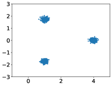
From Figure 1, we observe that the rdMC method deviates significantly from the conventional gradient-based MCMC techniques, such as Langevin dynamics. It visualizes the paths from a Gaussian distribution to a mixture of Gaussian distributions. It can be observed that Langevin dynamics, being solely driven by the gradient information of the target density , tends to get trapped in local regions, resulting in uneven sampling of the mixture of Gaussian distribution. More precisely, admits a small LSI constant due to the separation of the modes (Ma et al., 2019; Schlichting, 2019; Menz & Schlichting, 2014). Consequently, the convergence of conventional MCMC methods becomes notably challenging in such scenarios (Tosh & Dasgupta, 2014).
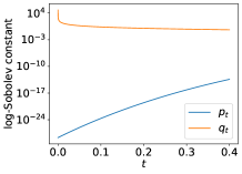
To better demonstrate the effect of our proposed SDE, we compute the LSI constant estimates for - case in Figure 2. Due to the shrinkage property of the forward process, the LSI constant of can be exponentially better than the original one. Meanwhile, for a , the LSI constant of is also well-behaved. In our algorithm, a well-conditioned LSI constant for both and reduces the computation overhead. Thus, we can choose a intermediate to connect those local modes and perform reverse SDE towards . rdMC can distribute samples more evenly across different modes and enjoy faster convergence in those challenging cases. Moreover, if the growth rate of is slower than the quadratic function (heavy tail), we can choose a large and use to estimate . Then, all have quadratic growth, which implies log-Sobolev property. These intuitions also explain why diffusion models excel in modeling complex distributions in high-dimensional spaces. We will provide the quantitative explanation in Section 4.
3.3 Algorithms for score estimation with
According to the expectation form of scores shown in Lemma 1, a detailed reverse sampling algorithm can be naturally proposed in Algorithm 1. Specifically, it can be summarized as the following steps: (1) choose proper and such that . This step can be done by either for large or performing the ULA for (Algorithm 3 in Appendix); (2) sample from a distribution that approximate (Step 4 of Algorithm 1); (3) follow with the approximated samples (Step 5 of Algorithm 1); (4) repeat until . After (4), we can also perform Langevin algorithm to fine-tune the steps when the gradient complexity limit is not reached.
The key of implementing Algorithm 1 is to estimate the scores via Step 4 with samples from . In what follows, we discuss the implementation that combines the importance weight sampling with the adjusted Langevin algorithm (ULA).
Importance weighted score estimator. We first consider importance sampling approach for estimating the score . From Eq. (4), we know that the key is to estimate:
and where Note that sampling from takes negligible computation resource. The main challenge is the sample complexity of estimating the two expectations.
Since is Gaussian with variance , we know that as long as is -Lipschitz, the sample complexity scales as for the resulting errors of the two mean estimators to be less than (Wainwright, 2019). However, the sample size required of the importance sampling method to achieve an overall small error is known to scale exponentially with the KL divergence between and (Chatterjee & Diaconis, 2018), which can depend on the dimension. In our current formulation, this is due to the fact that the true denominator can be as little as . As a result, to make the overall score estimation error small, the error tolerance and in turn the sample size required for estimating can scale exponentially with the dimension.
ULA score estimator. An alternative score estimator considers that the mean of the underlying distribution of these samples needs to sufficiently approach , which can be achieved by closing the gap of KL divergence or Wasserstein distance between and . Since the additional quadratic term shown in Eq. (4) helps improve a quadratic tail growth for , which implies the establishment of the isoperimetric condition. We expect the convergence can be achieved by performing the ULA on a sampling subproblem whose target distribution is . We provide the detailed implementation in Algorithm 2.
ULA score estimator with importance sampling initialization. Inspired by the previous estimators, we can combine the importance sampling approach with the ULA. In particular, we first implement the importance sampling method to form a rough score estimator. We then perform ULA at the mean estimator and obtain a refined accurate score estimate. Via this combination, we are able to efficiently obtain accurate score estimation by virtue of the ULA algorithm when is close to . When is close to , we are able to quickly obtain rough score estimates via the importance sampling approach. We discover empirically that this combination generally perform well when interpolates the two regimes (Figure 3 in Section 4).
4 Analyses and Examples of the rdMC Approach
In this section, we analyze the overall complexity of the rdMC via ULA inner loop estimation. Since the complexity of the importance sampling estimate is discussed in Section 3.3, we only consider Algorithm 1 with direct ULA sampling of rather than the smart importance sampling initialization to make our analysis clear.
To provide the analysis of the convergence of rdMC, we make the following assumptions.
-
[A1]
For all , the score is -Lipschitz.
-
[A2]
The second moment of the target distribution is upper bounded, i.e., .
These assumptions are standard in diffusion analysis to guarantee the convergence to the target distribution (Chen et al., 2022a). Specifically, Assumption [A1] governs the smoothness characteristics of the forward process, which ensure the feasibility of numerical discretization methods used for approximating the solution of continuous SDE. In addition, Assumption [A2] introduces essential constraints on the moments of the target distribution. These constraints effectively prevent an excessive accumulation of probability mass in the tail region, thereby ensuring a more balanced and well-distributed target distribution.
4.1 Outer loop complexity
According to Algorithm 1, the overall gradient complexity depends on the number of outer loops , as well as the complexity to achieve accurate score estimations (Line 5 in Algorithm 1). When the score is well-approximated and satisfies , the overall error in TV distance, , can be made by choosing a small . Under this condition, the number of outer loops satisfies , which shares the same complexity as that in diffusion analysis (Chen et al., 2022a; Lee et al., 2022; 2023). Such a complexity of the score estimation oracles is independent of the log-Sobolev (LSI) constant of the target density , which means that the isoperimetric dependence of rdMC is dominated by the subproblem of sampling from . Specifically, the following theorem demonstrates the conditions for achieving .
Theorem 1.
For any , assume that for some , as suggested in Algorithm 1, . If the OU process induced by satisfies Assumption [A1], [A2], and satisfies the log-Sobolev inequality (LSI) with constant (). We set
| (6) |
where is the number of samples to estimate the score, and is the KL error tolerence for the inner loop. With probability at least , Algorithm 1 converges in TV distance with error.
Therefore, the key points for the convergence of rdMC can be summarized as
-
•
The LSI of target distributions of sampling subproblems, i.e., is maintained.
-
•
The initialization of the reverse process is sufficiently close to .
4.2 Overall computation complexity
In this section, we consider the overall computation complexity of rdMC. Note that the LSI constants of depend on the properties of . As a result we consider more specific assumptions that bound the LSI constants for . In particular, we demonstrate the benefits of using for targets with infinite or exponentially large LSI constants. Compared with ULA, rdMC improves the gradient complexity, due to the improved LSI constant of over that of in finite . Even for heavy-tailed that does not satisfy the Poincaré inequality, target distributions of sampling subproblems, i.e., , can still preserve the LSI property, which helps rdMC to alleviate the exponential dimension dependence of gradient complexity for achieving TV distance convergence.
Specifically, Section 4.2.1 consider the case that the LSI constant of depend on the radius exponentially, which can usually be found in mixture models. Our proposed rdMC can reduce the exponent by a factor. Section 4.2.2 consider the case that is not LSI, but rdMC can create an LSI subproblem sequence which makes the dimension dependency polynomial.
We first provide an estimate for the LSI constant of under general Lipschitzness assumption [A1].
Lemma 2.
Under [A1], the LSI constant for in the forward OU process is when . This estimation indicate that when quadratic term dominate the log-density of , the log-Sobolev property is well-guaranteed.
4.2.1 Improving the LSI constant dependence for mixture models
Apart from Assumption [A1], [A2], we study the case where satisfies the following assumption:
-
[A3]
There exists , such that is -strongly convex when .
In this case, the target density admits an LSI constant which scales exponentially with the radius of the region of nonconvexity , i.e., , as shown in (Ma et al., 2019). This implies that if we draw samples from with ULA, the gradient complexity will have exponential dependency with respect to . However, in rdMC with suitable choices of and , the exponential dependency on is removed, which is a bottleneck for mixture models.
In the Proposition 1 below, we select values of and to achieve the desired level of accuracy. Notably, Lemma 2 suggest that we can choose a termination time to make the LSI constant of well-behehaved and is much simpler than . That is to say, rdMC can exhibit lower isoperimetric dependency compared to conventional MCMC techniques. Thus, We find that the overall computation complexity of rdMC reduces the dependency on .
Proposition 1.
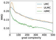
Example: Gaussian Mixture Model. We consider an example that
The LSI constant is (Ma et al., 2019; Schlichting, 2019; Menz & Schlichting, 2014), corresponding to the complexity of the target distribution. Tosh & Dasgupta (2014) prove that the lower bound iteration complexity by MCMC-based algorithm to sample from the Gaussian mixture scales exponentially with the squared distance between the two modes: . Note that rdMC is not a type of conventional MCMC. With importance sampling score estimator, the iteration complexity and samples at each step, the TV distance converges with error (Appendix B).
The computation overhead of the outer-loop process does not depend on . For the inner-loop score estimation we can choose to make the LSI constant of to be . We can perform ULA to initialize , which reduces the barrier between modes significantly. Specifically, the LSI constant of is , which improves the dependence on by a factor. Since this factor is on the exponent, the reduction is exponential.
Figure 3 is a demonstration for this example. We choose different to represent the change of in [A3]. We compare the convergence of Langevin Monte Carlo (LMC), Underdamped LMC (ULMC) and rdMC in terms of gradient complexity. As increases, we find that LMC fails to converge within a limited time. ULMC, with the introduction of velocity, can alleviate this situation. Notably, our algorithm can still ensure fast mixing for large . The inner loop is initialized with importance sampling mean estimator. Hyper-parameters and more results are provided in Appendix F.
4.2.2 Improving the dimension dependence in heavy-tailed target distributions
 |
 |
 |
 |
 |
 |
In this subsection, we study the case where satisfies Assumption [A1], [A2], and
-
[A4]
For any , we can find some satisfying is convex for . Without loss of generality, we suppose for some .
Assumption [A4] can be considered as a soft version of [A3]. Specifically, it permits the tail growth of the negative log-density to be slower than quadratic functions. This encompasses certain target distributions that fall outside the constraints of LSI and PI. Furthermore, given that the additional quadratic term present in Eq. (4) dominates the tail, satisfies LSI for all .
Lemma 3.
The uniform bound on the LSI constant enables us to estimate the score for any . We can consider cases that are free from the constraints on the properties of and let be sufficiently large. By setting at level, we can approximate with — the stationary distribution of the forward process. Furthermore, since are log-Sobolev, we can perform rdMC to sample from heavy-tailed in the absence of a log-Sobolev inequality. The explicit computational complexity of rdMC, needed to converge to any specified accuracy, is detailed in the subsequent proposition.
Proposition 2.
Example: Potentials with Sub-Linear Tails. We consider an example that
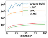
Lemma 5 demonstrates that this satisfies Assumption [A4] with . Moreover, these target distributions with sub-linear tails also satisfy weak Poincare inequality (wPI) introduced in Mousavi-Hosseini et al. (2023), in which the dimension dependence of ULA to achieve the convergence in TV distance is proven to be . Compared with this result, the complexity of rdMC shown in Proposition 2 has a lower dimension dependence when .
Conclusion. This paper presents a novel sampling algorithm based on the reverse SDE of the OU process. The algorithm efficiently generates samples by utilizing the mean estimation of a sub-problem to estimate the score function. It demonstrates convergence in terms of total variation distance and proves efficacy in general sampling tasks with or without isoperimetric conditions. The algorithm exhibits lower isoperimetric dependency compared to conventional MCMC techniques, making it well-suited for multi-modal and high-dimensional challenging sampling. The analysis provides insights into the complexity of score estimation within the OU process, given the conditional posterior distribution.
Acknowledgements
The research is partially supported by the NSF awards: SCALE MoDL-2134209, CCF-2112665 (TILOS). It is also supported in part by the DARPA AIE program, the U.S. Department of Energy, Office of Science, the Facebook Research Award, as well as CDC-RFA-FT-23-0069 from the CDC’s Center for Forecasting and Outbreak Analytics.
References
- Altschuler & Chewi (2023) Jason M Altschuler and Sinho Chewi. Faster high-accuracy log-concave sampling via algorithmic warm starts. arXiv preprint arXiv:2302.10249, 2023.
- Bakry et al. (2014) Dominique Bakry, Ivan Gentil, Michel Ledoux, et al. Analysis and geometry of Markov diffusion operators, volume 103. Springer, 2014.
- Berner et al. (2022) Julius Berner, Lorenz Richter, and Karen Ullrich. An optimal control perspective on diffusion-based generative modeling. arXiv preprint arXiv:2211.01364, 2022.
- Cattiaux et al. (2021) Patrick Cattiaux, Giovanni Conforti, Ivan Gentil, and Christian Léonard. Time reversal of diffusion processes under a finite entropy condition. arXiv preprint arXiv:2104.07708, 2021.
- Chafaï (2004) Djalil Chafaï. Entropies, convexity, and functional inequalities, on -entropies and -sobolev inequalities. Journal of Mathematics of Kyoto University, 44(2):325–363, 2004.
- Chatterjee & Diaconis (2018) Sourav Chatterjee and Persi Diaconis. The sample size required in importance sampling. Annals of Applied Probability, 28(2), 2018.
- Chen et al. (2023) Hongrui Chen, Holden Lee, and Jianfeng Lu. Improved analysis of score-based generative modeling: User-friendly bounds under minimal smoothness assumptions. In International Conference on Machine Learning, pp. 4735–4763. PMLR, 2023.
- Chen et al. (2022a) Sitan Chen, Sinho Chewi, Jerry Li, Yuanzhi Li, Adil Salim, and Anru R Zhang. Sampling is as easy as learning the score: theory for diffusion models with minimal data assumptions. arXiv preprint arXiv:2209.11215, 2022a.
- Chen et al. (2022b) Yongxin Chen, Sinho Chewi, Adil Salim, and Andre Wibisono. Improved analysis for a proximal algorithm for sampling. In Conference on Learning Theory, pp. 2984–3014. PMLR, 2022b.
- Cheng & Bartlett (2018) Xiang Cheng and Peter Bartlett. Convergence of langevin mcmc in kl-divergence. In Algorithmic Learning Theory, pp. 186–211. PMLR, 2018.
- Cheng et al. (2018) Xiang Cheng, Niladri S Chatterji, Peter L Bartlett, and Michael I Jordan. Underdamped langevin mcmc: A non-asymptotic analysis. In Conference on learning theory, pp. 300–323. PMLR, 2018.
- Chewi et al. (2021) Sinho Chewi, Murat A Erdogdu, Mufan Bill Li, Ruoqi Shen, and Matthew Zhang. Analysis of langevin monte carlo from poincaré to log-sobolev. arXiv preprint arXiv:2112.12662, 2021.
- Dalalyan (2017) Arnak Dalalyan. Further and stronger analogy between sampling and optimization: Langevin monte carlo and gradient descent. In Conference on Learning Theory, pp. 678–689. PMLR, 2017.
- Dong et al. (2023) Hanze Dong, Xi Wang, LIN Yong, and Tong Zhang. Particle-based variational inference with preconditioned functional gradient flow. In The Eleventh International Conference on Learning Representations, 2023. URL https://openreview.net/forum?id=6OphWWAE3cS.
- Durmus & Moulines (2019) Alain Durmus and Eric Moulines. High-dimensional bayesian inference via the unadjusted langevin algorithm. 2019.
- Dwivedi et al. (2018) Raaz Dwivedi, Yuansi Chen, Martin J Wainwright, and Bin Yu. Log-concave sampling: Metropolis-hastings algorithms are fast! In Conference on learning theory, pp. 793–797. PMLR, 2018.
- El Alaoui et al. (2022) Ahmed El Alaoui, Andrea Montanari, and Mark Sellke. Sampling from the sherrington-kirkpatrick gibbs measure via algorithmic stochastic localization. In 2022 IEEE 63rd Annual Symposium on Foundations of Computer Science (FOCS), pp. 323–334. IEEE, 2022.
- Eldan (2013) Ronen Eldan. Thin shell implies spectral gap up to polylog via a stochastic localization scheme. Geometric and Functional Analysis, 23(2):532–569, 2013.
- Eldan (2020) Ronen Eldan. Taming correlations through entropy-efficient measure decompositions with applications to mean-field approximation. Probability Theory and Related Fields, 176(3-4):737–755, 2020.
- Eldan (2022) Ronen Eldan. Analysis of high-dimensional distributions using pathwise methods. Proceedings of ICM, to appear, 2022.
- Erdogdu & Hosseinzadeh (2021) Murat A Erdogdu and Rasa Hosseinzadeh. On the convergence of langevin monte carlo: The interplay between tail growth and smoothness. In Conference on Learning Theory, pp. 1776–1822. PMLR, 2021.
- Freund et al. (2022) Yoav Freund, Yi-An Ma, and Tong Zhang. When is the convergence time of langevin algorithms dimension independent? a composite optimization viewpoint. Journal of Machine Learning Research, 23(214), 2022.
- Gross (1975) Leonard Gross. Logarithmic sobolev inequalities. American Journal of Mathematics, 97(4):1061–1083, 1975.
- Ho et al. (2020) Jonathan Ho, Ajay Jain, and Pieter Abbeel. Denoising diffusion probabilistic models. Advances in Neural Information Processing Systems, 33:6840–6851, 2020.
- Huang et al. (2021) Jian Huang, Yuling Jiao, Lican Kang, Xu Liao, Jin Liu, and Yanyan Liu. Schrödinger-föllmer sampler: sampling without ergodicity. arXiv preprint arXiv:2106.10880, 2021.
- Jerrum & Sinclair (1996) Mark Jerrum and Alistair Sinclair. The markov chain monte carlo method: an approach to approximate counting and integration. Approximation algorithms for NP-hard problems, pp. 482–520, 1996.
- Le Gall (2016) Jean-François Le Gall. Brownian motion, martingales, and stochastic calculus. Springer, 2016.
- Lee et al. (2021a) Holden Lee, Chirag Pabbaraju, Anish Sevekari, and Andrej Risteski. Universal approximation for log-concave distributions using well-conditioned normalizing flows. arXiv preprint arXiv:2107.02951, 2021a.
- Lee et al. (2022) Holden Lee, Jianfeng Lu, and Yixin Tan. Convergence for score-based generative modeling with polynomial complexity. arXiv preprint arXiv:2206.06227, 2022.
- Lee et al. (2023) Holden Lee, Jianfeng Lu, and Yixin Tan. Convergence of score-based generative modeling for general data distributions. In International Conference on Algorithmic Learning Theory, pp. 946–985. PMLR, 2023.
- Lee et al. (2021b) Yin Tat Lee, Ruoqi Shen, and Kevin Tian. Structured logconcave sampling with a restricted gaussian oracle. In Conference on Learning Theory, pp. 2993–3050. PMLR, 2021b.
- Liu & Wang (2016) Qiang Liu and Dilin Wang. Stein variational gradient descent: A general purpose bayesian inference algorithm. Advances in neural information processing systems, 29, 2016.
- Ma et al. (2019) Yi-An Ma, Yuansi Chen, Chi Jin, Nicolas Flammarion, and Michael I Jordan. Sampling can be faster than optimization. Proceedings of the National Academy of Sciences, 116(42):20881–20885, 2019.
- Ma et al. (2021) Yi-An Ma, Niladri S Chatterji, Xiang Cheng, Nicolas Flammarion, Peter L Bartlett, and Michael I Jordan. Is there an analog of Nesterov acceleration for gradient-based MCMC? Bernoulli, 27(3), 2021.
- Menz & Schlichting (2014) Georg Menz and André Schlichting. Poincaré and logarithmic sobolev inequalities by decomposition of the energy landscape. 2014.
- Montanari (2023) Andrea Montanari. Sampling, diffusions, and stochastic localization. arXiv preprint arXiv:2305.10690, 2023.
- Montanari & Wu (2023) Andrea Montanari and Yuchen Wu. Posterior sampling from the spiked models via diffusion processes. arXiv preprint arXiv:2304.11449, 2023.
- Mou et al. (2021) Wenlong Mou, Yi-An Ma, Martin J Wainwright, Peter L Bartlett, and Michael I Jordan. High-order langevin diffusion yields an accelerated mcmc algorithm. The Journal of Machine Learning Research, 22(1):1919–1959, 2021.
- Mousavi-Hosseini et al. (2023) Alireza Mousavi-Hosseini, Tyler Farghly, Ye He, Krishnakumar Balasubramanian, and Murat A Erdogdu. Towards a complete analysis of langevin monte carlo: Beyond poincar’e inequality. arXiv preprint arXiv:2303.03589, 2023.
- Neal (1993) Radford M Neal. Probabilistic inference using Markov chain Monte Carlo methods. Department of Computer Science, University of Toronto Toronto, ON, Canada, 1993.
- Poincaré (1890) Henri Poincaré. Sur les équations aux dérivées partielles de la physique mathématique. American Journal of Mathematics, pp. 211–294, 1890.
- Raginsky et al. (2017) Maxim Raginsky, Alexander Rakhlin, and Matus Telgarsky. Non-convex learning via stochastic gradient langevin dynamics: a nonasymptotic analysis. In Conference on Learning Theory, pp. 1674–1703. PMLR, 2017.
- Robert et al. (1999) Christian P Robert, George Casella, and George Casella. Monte Carlo statistical methods, volume 2. Springer, 1999.
- Rombach et al. (2022) Robin Rombach, Andreas Blattmann, Dominik Lorenz, Patrick Esser, and Björn Ommer. High-resolution image synthesis with latent diffusion models. In Proceedings of the IEEE/CVF Conference on Computer Vision and Pattern Recognition, pp. 10684–10695, 2022.
- Rothaus (1981) OS Rothaus. Diffusion on compact riemannian manifolds and logarithmic sobolev inequalities. Journal of functional analysis, 42(1):102–109, 1981.
- Schlichting (2019) André Schlichting. Poincaré and log–sobolev inequalities for mixtures. Entropy, 21(1):89, 2019.
- Song et al. (2020) Yang Song, Jascha Sohl-Dickstein, Diederik P Kingma, Abhishek Kumar, Stefano Ermon, and Ben Poole. Score-based generative modeling through stochastic differential equations. arXiv preprint arXiv:2011.13456, 2020.
- Tosh & Dasgupta (2014) Christopher Tosh and Sanjoy Dasgupta. Lower bounds for the gibbs sampler over mixtures of gaussians. In International Conference on Machine Learning, pp. 1467–1475. PMLR, 2014.
- Tzen & Raginsky (2019) Belinda Tzen and Maxim Raginsky. Theoretical guarantees for sampling and inference in generative models with latent diffusions. In Conference on Learning Theory, pp. 3084–3114. PMLR, 2019.
- Vargas et al. (2023a) Francisco Vargas, Will Grathwohl, and Arnaud Doucet. Denoising diffusion samplers. arXiv preprint arXiv:2302.13834, 2023a.
- Vargas et al. (2023b) Francisco Vargas, Andrius Ovsianas, David Fernandes, Mark Girolami, Neil D Lawrence, and Nikolas Nüsken. Bayesian learning via neural schrödinger–föllmer flows. Statistics and Computing, 33(1):3, 2023b.
- Vargas et al. (2023c) Francisco Vargas, Teodora Reu, and Anna Kerekes. Expressiveness remarks for denoising diffusion based sampling. In Fifth Symposium on Advances in Approximate Bayesian Inference, 2023c.
- Vempala & Wibisono (2019) Santosh Vempala and Andre Wibisono. Rapid convergence of the unadjusted langevin algorithm: Isoperimetry suffices. Advances in neural information processing systems, 32, 2019.
- Villani (2021) Cédric Villani. Topics in optimal transportation, volume 58. American Mathematical Soc., 2021.
- Wainwright (2019) Martin J Wainwright. High-dimensional statistics: A non-asymptotic viewpoint, volume 48. Cambridge university press, 2019.
- Zhang et al. (2023) Dinghuai Zhang, Ricky Tian Qi Chen, Cheng-Hao Liu, Aaron Courville, and Yoshua Bengio. Diffusion generative flow samplers: Improving learning signals through partial trajectory optimization. arXiv preprint arXiv:2310.02679, 2023.
Appendix A Proof Sketch
For better understanding for our paper, we provide a proof sketch as below.
Lemma 1 is a direct result of Bayes theorem (Appendix C.1), which is the main motivation of our algorithm, that estimate the score with samples from .
Our main contribution is to prove the convergence and evaluate the complexity of Algorithm 1, where the inner loop is performed by Algorithm 2.
Our analysis is based on the TV distance111Please refer to Table 1 for the notation definitions., where we use data-processing inequality, triangle inequality, and Pinsker’s inequality (refer to Eq. (19) for details) to provide the upper bound as below
where Term 1 is the error between and and Team 2 is the score estimation loss of the whole trajectory.
Theorem 1 considers the case that all is log-Sobolev with constant (), where the log-Sobolev constants can further be estimated with additional assumptions on .
By definition,
where Term 2 is defined by an integration.
To bound the error between integration and discretized algorithm, we have Lemma 7 that when
| (7) |
Note that the can be controlled by
and
where is the estimated inner loop distribution by ULA.
Lemma 8 provide the concentration for Term 2.1.
We also have
where the KL divergence is controlled by the convergence of ULA (Lemma 9). Thus, the desired convergence can be obtained.
Note that Theorem 1 is based on the fact that all are log-Sobolev. So we aim to estimate the log-Sobolev constants for every .
When is strongly convex outside a ball with radius , we can derive that can reduce the radius so that improve the log-Sobolev constant. Thus, we can choose proper where has larger log-Sobolev constant than and are strongly convexity so that the log-Sobolev constants are independent of , which makes the algorithm mix fast.
For more general distributions without log-Sobolev constant, Lemma 10 provide the log-Sobolev constant the whole trajectory, so that the computation complexity can be obtained.
Appendix B Notations and discussions
B.1 Algorithm
B.2 Notations
According to Cattiaux et al. (2021), under mild conditions in the following forward process the reverse process also admits an SDE description. If we fix the terminal time and set the process satisfies the SDE where the reverse drift satisfies the relation In this condition, the reverse process of SDE (1) is as follows
| (8) |
Thus, once the score function is obtained, the reverse SDE induce a sampling algorithm. To obtain the particles along SDE (8), the first step is to initialize the particle with a tractable starting distribution. In real practice, it is usually hard to sample from the ideal initialization directly due to its unknown properties. Instead, we sample from an approximated distribution . For large , is chosen for approximating as their gap can be controlled. For the iteration, we utilize the numerical discretization method, i.e., DDPM Ho et al. (2020), widely used in diffusion models’ literature. Different from ULA, DDPM divides SDE (8) by different time segments, and consider the following SDE for each segment
| (9) |
to discretize SDE (8). Suppose we obtain to approximate at each iteration. Then, we obtain the SDE 2 for practical updates of particles.
Reiterate of Algorithm 1
Once the score function can be estimated, the sampling algorithm can be presented. The detailed algorithm is described in Algorithm 1. By following these steps, our proposed algorithm efficiently addresses the given problem and demonstrates its effectiveness in practical applications. Specifically, we summarize our algorithm as below: (1) choose proper and proper such that . This step can be done by either for large or performing the Langevin Monte Carlo for ; (2) sample from ; (3) sample from a distribution that approximate ; (4) update with the approximated samples. This step can be done by Langevin Monte Carlo inner loop, as is explicit; (5) repeat (3) and (4) until . After (5), we can also perform Langevin algorithm to fine-tune the steps when the gradient complexity limit is not reached. The main algorithm as Algorithm 1.
Here, we reiterate our notation in Table 1 and the definition of log-Sobolev inequality as follows.
Definition 1.
(Logarithmic Sobolev inequality) A distribution with density function satisfies the log-Sobolev inequality with a constant if for all smooth function with ,
| (10) |
| Symbols | Description |
| The density function of the centered Gaussian distribution, i.e., . | |
| The target density function (initial distribution of the forward process) | |
| The forward process, i.e., SDE (1) | |
| The density function of , i.e., | |
| The density function of stationary distribution of the forward process. | |
| The ideal reverse process, i.e., SDE (8) | |
| The density function of , i.e., and | |
| The law of the ideal reverse process SDE (8) over the path space . | |
| The reverse process following from SDE (9) | |
| The density function of , i.e., | |
| The practical reverse process following from SDE (2) with initial distribution | |
| The density function of , i.e., | |
| The law of the reverse process over the path space . | |
| The reverse process following from SDE (2) with initial distribution | |
| The density function of , i.e., | |
| The law of the reverse process over the path space . |
Besides, there are many constants used in our proof. We provide notations here to prevent confusion.
| Constant | Value | Constant | Value |
B.3 Examples
Lemma 4.
(Proof of the Gaussian Mixture example) The iteration and sample complexity of rdMC with importance sampling estimator is .
Proof.
Similar to Eq. (19) in Theorem 1, we have
| (11) |
by using data-processing inequality, triangle inequality, and Pinsker’s inequality.
To ensure Term 1 controllable, we choose .
For Term 2,
By Lemma 7,
| (12) |
Thus, the iteration complexity of the RDS algorithm is when the score estimator error is , which is controlled by concentration inequalities.
For time , since we have and is sub-Gaussian, the density is also sub-Gaussian with variance .
We have
For Gaussian mixture model, is -Lipschitz and function is -Lipschitz smooth, is -Lipschitz.
For time , the variance is .
Assume that the expectation and the estimator of is and . The expectation and the estimator of is and
We choose , .
If , with probability , the error of the estimator is at most .
Moreover, if we choose the inner loop iteration to estimate the posterior. We can start from some , and estimate initially.
Specifically, for the Gaussian mixture, we can get a tighter log-Sobolev bound. For time , we have , which indicate the log-Sobolev constant, . Considering the smoothness, we have
When we choose , The estimation of needs iterations, which improves the original . ∎
Lemma 5.
Suppose the negative log density of target distribution satisfies
where .
Proof.
Consider the Hessian of , we have
If we require , it has
It means if we choose and ∎
B.4 More discussion about previous works
Recent studies have underscored the potential of diffusion models, exploring their integration across various domains, including approximate Bayesian computation methods. One line of research (Vargas et al., 2023a; Berner et al., 2022; Zhang et al., 2023; Vargas et al., 2023c; b) involves applying reverse diffusion in the VI framework to create posterior samplers by neural networks. These studies have examined the conditional expected form of the score function, similar to Lemma 1. Such score-based VI algorithms have shown to offer improvements over traditional VI. However, upon adopting a neural network estimator, VI-based algorithms are subject to an inherent unknown error.
Other research (Tzen & Raginsky, 2019; Chen et al., 2022a) has also delved into the characteristics of parameterized diffusion-like processes under assumed error conditions. Yet, the comparative advantages of diffusion models against MCMC methods and the computational complexity involved in learning the score function are not well-investigated. This gap hinders a straightforward comparison with Langevin-based dynamics.
Another related work is the Schrödinger-Föllmer Sampler (SFS) (Huang et al., 2021), which also tend to estimate the drift term with non-parametric estimators. The main difference of the proposed algorithm is that SFS leverages Schrödinger-Föllmer process. In this process, the target distribution is transformed into a Dirac delta distribution. This transformation often results in the gradient becoming problematic when closely resembles a delta distribution, posing challenges for maintaining the Lipschitz continuity of the drift term. Huang et al. (2021); Tzen & Raginsky (2019) note that the assumption holds when both and its gradient are Lipschitz continuous, and the former is bounded below by a positive value. However, this condition may not be met when the variance of exceeds 1, limiting its general applicability in the Schrödinger-Föllmer process. The comparison of SFS with traditional MCMC methods under general conditions remains an open question. However, given that the of the OU process represents a smooth distribution – a standard Gaussian, the requirement for the Lipschitz continuity of is much weaker, as diffusion analysis suggested (Chen et al., 2022a; 2023). Additionally, Lee et al. (2021a) indicated that -smoothness in log-concave implies the smoothness in . Moreover, the SFS algorithm considers the importance sampling estimator and the error analysis is mainly based on the Gaussian mixture model. As we mentioned in our Section 3.3, importance sampling estimator would suffer from curse of dimensionality in real practice. Our ULA-based analysis can be adapted to more general distributions for both ill-behaved LSI and non-LSI distributions. In a word, our proposed rdMC provide the complexity for general distributions and SFS is more task specific. It remains open to further investigate the complexity for SFS-like algorithm, which can be interesting future work. Moreover, it is also possible to adapt the ULA estimator idea to SFS.
Our approach, stands as an asymptotically exact sampling algorithm, akin to traditional MCMC methods. It allows us to determine an overall convergence rate that diminishes with increasing computational complexity, enabling a direct comparison of complexity with MCMC approaches. The main technique of our algorithm is to analyze the complexity of the score estimation with non-parametric algorithm and we found the merits of the proposed one compared with MCMC. Our theory can also support the diffusion-based VI against Langevin-based ones.
Appendix C Main Proofs
C.1 Proof of Lemma 1
Proof.
When the OU process, i.e., Eq. 1, is selected as our forward path, the transition kernel of has a closed form, i.e.,
In this condition, we have
Plugging this formulation into the following equation
we have
| (13) | ||||
where the density function is defined as
Hence, the proof is completed. ∎
C.2 Proof of Lemma 2 and 3
Lemma 6.
(Proposition 1 in Ma et al. (2019)) For , where is -strongly convex outside of a region of radius and -Lipschitz smooth, the log-Sobolev constant of
C.3 Proof of Main Theorem
Proof.
We have
| (15) | ||||
where the first and the third inequalities follow from data-processing inequality, the second inequality follows from the triangle inequality, and the last inequality follows from Pinsker’s inequality.
For Term 2,
By Lemma 7,
| (16) |
According to Eq. 4, for each term of the summation, we have
For each , we have
| (17) | ||||
where we denote denote the underlying distribution of output particles of the auxiliary sampling task.
For , we denote an optimal coupling between and to be
Hence, we have
| (18) | ||||
where the first inequality follows from Jensen’s inequality, the second inequality follows from the Talagrand inequality and the last inequality follows from
when .
∎
C.4 Proof of the main Propositions
Proof.
By Eq. (19), we have the upper bound for
| (19) |
We aim to upper bound these two terms in our analysis.
Errors from the forward process
For Term 1 of Eq. 19, we can either choose or choose large with .
If we choose , we have
where the inequality follows from Lemma 21. By requiring
we have . To simplify the proof, we choose as its lower bound.
If we choose , then the iteration complexity depend on the log-Sobolev constant of . In (Ma et al., 2019), it is demonstrated that any distribution satisfying Assumptions [A1] and [A3] has a log-Sobolev constant of , which scales exponentially with the radius .
Considering the , we have
Assume that the density of is ,
Assume that and Assumption [A3] holds,
We have outside a ball with , the negative log-density is strongly convex. By Lemma 16, the final log-Sobolev constant is
Errors from the backward process
Without loss of generality, we consider the Assumption [A4] case, where has been split to two intervals. The Assumption [A3] case can be recognized as the first interval of Assumption [A4]. For Term 2, we first consider the proof when Novikov’s condition holds for simplification. A more rigorous analysis without Novikov’s condition can be easily extended with the tricks shown in (Chen et al., 2022a). Considering Corollary 2, we have
| (20) | ||||
where .
We also have
| (21) |
following Lemma 7 by choosing the step size of the backward path satisfying
| (22) |
To simplify the proof, we choose as its upper bound. Plugging Eq. 32 into Eq. 20, we have
Besides, due to Lemma 10, we have
with a probability at least by requiring an
gradient complexity. Hence, we have
which implies
| (23) |
Hence, the proof is completed.
∎
Appendix D Important Lemmas
Lemma 7.
(Errors from the discretization) With Algorithm 1 and notation list 1, if we choose the step size of outer loop satisfying
then for we have
Proof.
According to the choice of , we have . With the transition kernel of the forward process, we have the following connection
| (24) | ||||
where the last equation follows from setting . We should note that
is also a density function. For each element , we have
where the inequality follows from the triangle inequality and Eq. 24. For the first term, we have
| (25) | ||||
For the second term, the score is -smooth. Therefore, with Lemma 13 and the requirement
we have
| (26) | ||||
Due to the range , we have the following inequalities
Thus, Eq. 25 and Eq. 26 can be reformulated as
| (27) | ||||
and
which is equivalent to
| (28) | ||||
Without loss of generality, we suppose , combining Eq. 27 and Eq. 28, we have the following bound
| (29) | ||||
Besides, we have
| (30) | ||||
where the last inequality with Lemma 14 and Lemma 15. To diminish the discretization error, we require the step size of backward sampling, i.e., satisfies
Specifically, if we choose
we have
| (31) |
Hence, the proof is completed.
∎
Lemma 8.
For each inner loop, we denote and to be the underlying distribution of output particles and the target distribution, respectively, where satisfies LSI with constant . When we set the step size of outer loops to be , by requiring
we have
where
Proof.
For each inner loop, we abbreviate the target distribution as , the initial distribution as . Then the iteration of the inner loop is presented as
We suppose the underlying distribution of the -th iteration to be . Hence, we expect the following inequality
is established, where . In this condition, we have
| (33) | ||||
To simplify the notations, we set
Then, we have
| (34) | ||||
Consider the first term, we have the following relation
| (35) | ||||
where the last inequality follows from
| (36) | ||||
and
deduced by Lemma 23. By requiring
| (37) |
in Eq. 35, we have
| (38) | ||||
According to Lemma 16, the LSI constant of
is . Besides, considering the function is -Lipschitz because
we have
| (39) |
due to Lemma 18. Plugging Eq. 39 and Eq. 38 into Eq. 34 and Eq. 33, we have
| (40) | ||||
Besides, we have
Suppose the optimal coupling of and is , then we have
where the last inequality follows from Eq. 36 and Lemma 23. By requiring , we have
Combining this result with Eq. 40, we have
By requiring
| (41) | ||||
we have
Combining the choice of and the gap between and in Eq. 37 and Eq. 41, we have
| (42) |
Without loss of generality, we suppose , due to the range of as follows
we obtain the sufficient condition for achieving Eq. 42 is
Hence, the proof is completed. ∎
Lemma 9.
Proof.
According to the fact that the LSI constant of is , then we have
Because is a high-dimensional Gaussian, its mean value satisfies . Besides, we have
According to Lemma 20, satisfies the log-Sobolev inequality (and the Poincaré inequality). Follows from Lemma 23, we have
Hence, we have
and the proof is completed. ∎
Lemma 10.
Proof.
To upper bound it more precisely, we divide the backward process into two stages.
Stage 1: when .
It implies the iteration satisfies
| (43) |
In this condition, we set
| (44) |
Hence, we can reformulate as
According to Assumption [A4], we know part 1 and part 2 are both strongly convex outside the ball with radius . With Lemma 22, the function is -strongly convex outside the ball. Besides, the gradient Lipschitz constant of can be upper bounded as
where the last inequality follows from the choice of in the stage.
When the total time satisfies , we have
The second inequality follows from Assumption [A4], and the last inequality follows from the setting without loss of generality.
| (45) |
For , due to Lemma 8, if we set the step size of outer loop to be
the sample number of each iteration satisfies
and the accuracy of the inner loop meets
| (46) | ||||
when . In this condition, we have
| (47) | ||||
where denotes the underlying distribution of output particles of the -th inner loop. To achieve
Lemma 19 requires the step size to satisfy
and the iteration number meets
where denotes the initial distribution of the -th inner loop. By choosing to be its upper bound and the initial distribution of -th inner loop to be
we have
with Lemma 9 and Eq. 45. It implies the iteration number of inner loops to be required as
when and without loss of generality.
A sufficient condition to obtain is to make the following inequality establish
which will be dominated by Eq. 46 in almost cases obviously.
Stage 2: when .
We have the LSI constant for this stage. It is a constant level LSI constant, which mean we should choose the sample and the iteration number similar to Stage 1. Therefore, for , by requiring
and
| (50) | ||||
In this condition, we have
| (51) | ||||
where denotes the underlying distribution of output particles of the -th inner loop. To achieve
Lemma 19 requires the step size to satisfy
and the iteration number meets
where denotes the initial distribution of the -th inner loop. By choosing to be its upper bound and the initial distribution of -th inner loop to be
we have
with Lemma 9 and Eq. 14. It implies the iteration number of inner loops to be required as
when and without loss of generality.
For , we denote an optimal coupling between and to be
Hence, we have
| (52) | ||||
where the first inequality follows from Jensen’s inequality, the second inequality follows from the Talagrand inequality and the last inequality follows from
when . Therefore, a sufficient condition to obtain is to make the following inequality establish
which will be dominated by Eq. 50 in almost cases obviously.
Hence, combining Eq. 17, Eq. 51 and Eq. 52, there is
| (53) |
with a probability at least which is obtained by uniformed bound. We require the gradient complexity in this stage will be
| (54) | ||||
where the last inequality follows from Lemma 14. Combining Eq. 49 and Eq. 54, we know the total gradient complexity will be less than
Hence the proof is completed. ∎
Appendix E Auxiliary Lemmas
Lemma 11.
(Lemma 11 of Vempala & Wibisono (2019)) Assume is -smooth. Then .
Lemma 12.
(Girsanov’s theorem, Theorem 5.22 in Le Gall (2016)) Let and be two probability measures on path space . Suppose under , the process follows
Under , the process follows
We assume that for each , is a non-singular diffusion matrix. Then, provided that Novikov’s condition holds
we have
Corollary 2.
Lemma 13.
(Lemma C.11 in Lee et al. (2022)) Suppose that is a probability density function on , where is -smooth, and let be the density function of . Then for , it has
Lemma 14.
Lemma 15.
Proof.
According to the forward process, we have
where the third inequality follows from Holder’s inequality and the last one follows from Lemma 14. Hence, the proof is completed. ∎
Lemma 16.
(Corollary 3.1 in Chafaï (2004)) If satisfy LSI with constants , respectively, then satisfies LSI with constant .
Lemma 17.
Let be a real random variable. If there exist constants such that for all then
Proof.
According to the non-decreasing property of exponential function , we have
The first inequality follows from Markov inequality and the second follows from the given conditions. By minimizing the RHS, i.e., choosing , the proof is completed. ∎
Lemma 18.
If satisfies a log-Sobolev inequality with log-Sobolev constant then every -Lipschitz function is integrable with respect to and satisfies the concentration inequality
Proof.
According to Lemma 17, it suffices to prove that for any -Lipschitz function with expectation ,
To prove this, it suffices, by a routine truncation and smoothing argument, to prove it for bounded, smooth, compactly supported functions such that . Assume that is such a function. Then for every the log-Sobolev inequality implies
which is written as
With the notation and , the above inequality can be reformulated as
where the last step follows from the fact . Dividing both sides by gives
Denoting that the limiting value , we have
which implies that
Then the proof can be completed by a trivial argument of Lemma 17. ∎
Lemma 19.
(Theorem 1 in Vempala & Wibisono (2019)) Suppose satisfies LSI with constant and is -smooth. For any with , the iterates of ULA with step size satisfy
Thus, for any , to achieve , it suffices to run ULA with step size
for
Lemma 20.
(Variant of Lemma 10 in Cheng & Bartlett (2018)) Suppose is -strongly convex function, for any distribution with density function , we have
By choosing for the test function and , we have
which implies satisfies -log-Sobolev inequality.
Lemma 21.
Using the notation in Table. 1, for each , the underlying distribution of the forward process satisfies
Proof.
Consider the Fokker–Planck equation of the forward process, i.e.,
we have
It implies that the stationary distribution is
| (55) |
Then, we consider the KL convergence of , and have
| (56) | ||||
According to Proposition 5.5.1 of Bakry et al. (2014), if is a centered Gaussian measure on with covariance matrix , for every smooth function on , we have
For the forward stationary distribution Eq. 55, we have . Hence, by choosing , we have
Plugging this inequality into Eq. 56, we have
Integrating implies the desired bound,i.e.,
∎
Lemma 22.
Suppose and is -strongly convex for . That means (and ) is convex on . Specifically, we require that , any convex combination of with satisfies
Then, we have is -strongly convex for .
Proof.
We define . Hence, by considering and its convex combination of with , we have
Hence, the proof is completed. ∎
Lemma 23.
Suppose is a distribution which satisfies LSI with constant , then its variance satisfies
Proof.
It is known that LSI implies Poincaré inequality with the same constant (Rothaus, 1981; Villani, 2021; Vempala & Wibisono, 2019), which can be derived by taking in Eq. (10). Thus, for -LSI distribution , we have
for all smooth function .
In this condition, we suppose , and have the following equation
where is defined as and is a one-hot vector ( the -th element of is others are ).
Combining this equation and Poincaré inequality, for each , we have
By combining the equation and inequality above, we have
Hence, the proof is completed. ∎
Appendix F Empirical Results
F.1 Experiment settings and more empirical results
We choose particles in the experiments and use MMD (with RBF kernel) as the metric. We choose . We use , , or iterations to approximate chosen by the corresponding problem. The inner loop is initialized with importance sampling mean estimator by particles. The inner iteration and inner loop sample-size are chosen from . The outer learning rate is chosen from . When the algorithm converges, we further perform LMC until the limit of gradient complexity. Note that the gradient complexity is evaluated by the product of outer loop and inner loop.
 |
 |
 |
 |
 |
 |
 |
 |
 |
 |
 |
 |
F.2 More Investigation on Ill-behaved Gaussian Case
Figure 6 demonstrate the differences between Langevin dynamics and the OU process in terms of their trajectories. The former utilizes the gradient information of the target distribution , to facilitate optimization. However, it converges slowly in directions with small gradients. On the other hand, the OU process constructs paths with equal velocities in each direction, thereby avoiding the influence of gradient vanishing directions. Consequently, leveraging the reverse process of the OU process is advantageous for addressing the issue of uneven gradient sampling across different directions.
 |
 |
 |
 |
| Langevin | OU process |
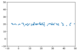
In order to further demonstrate the effectiveness of our algorithm, we conducted additional experiments comparing the Langevin dynamics with our proposed method in our sample scenarios. To better highlight the impacts of different components, we chose the -dimensional ill-conditioned Gaussian distribution (shown in Figure 7) as the target distribution to showcase this aspect. In this setting, we obtained an oracle sampler for , enabling us to conduct a more precise experimental analysis of the sample complexity.
 |
 |
| Initial distribution | Target distribution |
Figure 8 illustrates the distributions of samples generated by the LMC algorithm at iterations 10, 100, 1000, and 10000. It can be observed that these distributions deviate from the target distribution.
 |
 |
 |
 |
Figure 9 demonstrates the performance of the rdMC algorithm in the scenario of infinite samples, revealing its significantly superior convergence compared to the LMC algorithm.
 |
 |
 |
 |
Figure 10 showcases the convergence of the rdMC algorithm in estimating the score under different sample sizes. It can be observed that our algorithm is not sensitive to the sample quantity, demonstrating its robustness in practical applications.
 |
 |
| sample size | sample size |
 |
 |
| sample size | sample size |
Figure 11 illustrates the convergence behavior of the rdMC algorithm with an inexact solver. It can be observed that even when employing LMC as the solver for the inner loop, the final convergence of our algorithm surpasses that of the original LMC. This is attributed to the insensitivity of the algorithm to the precision of the inner loop when is large. Additionally, when is small, the log-Sobolev constant of the inner problem is relatively large, simplifying the problem as a whole and guiding the samples towards the target distribution through the diffusion path.
 |
 |
| inner loop | inner loop |
 |
 |
| inner loop | inner loop |
F.3 Sampling from high-dimensional distributions
To validate the dimensional dependency of rdMC algorithm, we consider to extend our Gaussian mixture model experiments.
In the log-Sobolev distribution context (see Section 4.2.1), both the Langevin-based algorithm and our proposed method exhibit polynomial dependence on dimensionality. However, the log-Sobolev constant grows exponentially with radius , which is the primary influencing factor. This leads to behavior akin to the 2-D example presented earlier. A significant limitation of the Langevin-based algorithm is its inability to converge within finite time for large values, in contrast to the robustness of our algorithm. In higher-dimensional scenarios (e.g., for and ), we observe a notable decrease in rdMC performance after approximately 100 computations. This decline may stem from the kernel-based computation of MMD, which tends to be less sensitive in higher dimensions. For these large cases, LMC and ULMC fails to converge in finite time. Overall, Figure 12 exhibits trends consistent with Figure 3, corroborating our theoretical findings.
 |
 |
 |
 |
 |
 |
 |
 |
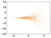
For heavy-tail distribution (refer to Section 4.2.2), the complexity of both rdMC and MCMC are quite high, so it is not feasible to sample from them in limited time. Nonetheless, as our algorithm only has the polynomial dependency of , but the Langevin-based algorithms have exponential dependency with respect to , we may have more advantages. For example, we can use the moment demonstrate the similarity of different distributions. To illustrate the phenomenon, we consider the extreme case – Cauchy distribution222The mean of Cauchy distribution does not exist. We use the case for better heavy-tail demonstration.. According to Figure 13, rdMC has better approximation for the true distribution and the approximation gap increases with respect to dimension.
 |
 |
 |
| moment | moment | moment |
F.4 Discussion on the choice of
Note that different may have impacts on the algorithm. In this subsection, we discuss the impact of choice of and try to make a clear demonstration for the influence in real practice.
Practically, selecting determines the initial distribution for reverse diffusion. While any choice can achieve convergence, the computational complexity varies with different values. According to Figure 14, we can notice that with the increase of , the modes of tend to merge to a single mode, and the speed is exponentially fast (Lemma 21). Even with , the dis-connectivity of modes can be alleviated significantly. Thus, the choice of is not sensitive when choosing from to .
 |
 |
 |
 |
However, when choosing too small or too large , there would be some consequence:
-
•
If is too small, the approximation of would be extremely hard. For example, if , the algorithm would be similar to Langevin algorithm;
-
•
If is too large, it would be wasteful to transport from to since the distribution in this interval is highly homogeneous333It is possible to consider varied step size scheduling, which can be interesting future work..
In summary, aside from the scenario, our algorithm exhibits insensitivity to the choice of (or ). Selecting an appropriate can reduce computational demands when using a constant step size schedule.
F.5 Neal’s Funnel
Neal’s Funnel is a classic demonstration of how traditional MCMC methods struggle with convergence unless specific parameterization strategies are employed. We further investigate the performance of our algorithm for this scenario. As indicated in Figure 15, our method demonstrates more rapid convergence compared to Langevin-based MCMC approaches. Additionally, Figure 16 reveals that while LMC lacks efficient exploration capabilities, ULMC fails to accurately represent density. This discrepancy stems from incorporating momentum/velocity. Our algorithm strikes an improved balance between exploration and precision, primarily due to the efficacy of the reverse diffusion path, thereby enhancing convergence speed.
 |
 |
 |
 |
 |
 |
 |
| Ground Truth | LMC | ULMC | rdMC |