Rethinking PGD Attack: Is Sign Function Necessary?
Abstract
Neural networks have demonstrated success in various domains, yet their performance can be significantly degraded by even a small input perturbation. Consequently, the construction of such perturbations, known as adversarial attacks, has gained significant attention, many of which fall within "white-box" scenarios where we have full access to the neural network. Existing attack algorithms, such as the projected gradient descent (PGD), commonly take the sign function on the raw gradient before updating adversarial inputs, thereby neglecting gradient magnitude information. In this paper, we present a theoretical analysis of how such sign-based update algorithm influences step-wise attack performance, as well as its caveat. We also interpret why previous attempts of directly using raw gradients failed. Based on that, we further propose a new raw gradient descent (RGD) algorithm that eliminates the use of sign. Specifically, we convert the constrained optimization problem into an unconstrained one, by introducing a new hidden variable of non-clipped perturbation that can move beyond the constraint. The effectiveness of the proposed RGD algorithm has been demonstrated extensively in experiments, outperforming PGD and other competitors in various settings, without incurring any additional computational overhead. The codes is available in https://github.com/JunjieYang97/RGD.
1 Introduction
Neural network has been widely adopted in many areas, e.g., computer vision (Krizhevsky et al., 2012; He et al., 2016) and natural language processing (Hochreiter and Schmidhuber, 1997). Generally, a well-trained neural network can make very accurate prediction when classifying image classes. However, existing works (Goodfellow et al., 2015; Madry et al., 2018; Zhang et al., 2020, 2021) have shown that merely tiny perturbations of the neural network input, which would not affect human judgment, might cause significant mistakes for the network output. These perturbations can be intentionally generated using various algorithms, usually referred to as adversarial attacks. Adversarial attacks are commonly categorized into white-box attacks and black-box attacks. In white-box attacks, we have access to all neural network parameters, allowing us to exploit this information (e.g., through back-propagation) to generate adversarial inputs. In contrast, the neural network architectures are inaccessible in the scenario of black-box attacks, and one can only test different inputs and their corresponding outputs to identify successful adversarial examples.
This work focuses exclusively on the white-box scenario, particularly for the norm-based projected gradient descent (PGD) (Madry et al., 2018) attack. In norm attacks, the learned perturbation is constrained within an -ball, ensuring that the absolute magnitudes of all pixel values do not exceed . Under these constraints, most white-box algorithms employ the "signed gradient" to maximize the perturbation values and approach the boundary, thereby generating stronger attacks. For instance, the Fast Gradient Sign Method (FGSM) (Goodfellow et al., 2015) initially introduces the sign operation for one-step perturbation update. Subsequently, Madry et al. (2018) proposes the PGD to iteratively update the perturbation using the signed gradient. Following-up PGD-based approaches, such as MIM (Dong et al., 2018) and Auto-Attack (Croce and Hein, 2020), unanimously follow the practice of using the sign function. Previous work (Agarwal et al., 2020) has empirically demonstrated that the "signed gradient" significantly outperforms the raw gradient in FGSM context. However, the signed gradient, compared to the raw gradient, abandons magnitude information in PGD, which may compromise the adversary information too. This motivates the following questions:
-
Despite the loss of gradient value information, sign-based attacks remain the preferred choice in norm scenarios. What are the critical factors in determining the quality of perturbations in PGD? Why does the raw gradient fail to generate more effective adversarial attacks?
Note that the raw gradient is found effective in contexts. For instance, the C&W (Carlini and Wagner, 2017) attack, a widely used algorithm, utilizes the raw gradient and incorporates constraint terms and variable changes for adversarial attacks. Therefore, more pertinent questions arise:
-
Why does the "signed gradient" appear necessary in attacks? What are the pros and cons of the sign function? Can we achieve more general attack success (including ) without the “sign" operation, and can that even outperform signed gradients?
1.1 Main Contributions
This work rigorously analyzes how the perturbation update method affects the adversarial quality and further empirically shows why raw gradient is not favored in the current PGD algorithm. Moreover, we propose a new raw gradient-based algorithm that outperforms vanilla PGD across various scenarios without introducing any extra computational cost.
In this study, our first objective is to theoretically characterize the effect of update mechanisms on adversarial samples at each step. We observe that a stronger attack in the previous step, or a larger perturbation change, leads to a greater attack improvement in the subsequent step. Furthermore, our empirical observations reveal that in the later update steps, vanilla PGD, which employs the sign function, exhibits a larger change in perturbation compared to raw gradient-based PGD. Such a larger change facilitates more pixels approaching the boundary, indicating a stronger attack update based on the theoretical results. This explains the preference for using the signed gradient in PGD.
Next, we point out that the failure of the raw gradient in PGD is not only due to the insufficient update on its own, but also attributed to the clipping design. In PGD, all perturbations are clipped within the ball per step. This design results in the loss of significant magnitude information for the raw gradient update, particularly when most pixels approach the boundary. Instead, we introduce a new hidden variable of non-clipped perturbation for updating. In this way, the norm-based adversarial attack, a constrained optimization problem, is transformed into an unconstrained optimization problem, where the proposed hidden variable is allowed to surpass the boundary. Extensive experiments further demonstrate that our proposed method significantly improves the performance of raw update-based PGD and even outperforms vanilla PGD, without incurring additional computational overhead.
2 Related Works
Adversarial robustness has been explored in recent years. Szegedy et al. (2013) were the first to mention that imperceptible perturbations can cause networks to misclassify images. Then, based on gradients with respect to the input, Goodfellow et al. (2015) proposed the one-step FGSM for generating adversarial examples. Furthermore, iterative-based adversarial attacks such as BIM (Kurakin et al., 2018) and PGD (Madry et al., 2018) have been proposed for white-box attacks. The difference between these algorithms lies in whether they adopt random initialization or not. The C&W attack (Carlini and Wagner, 2017) introduced a regularized loss parameterized by and demonstrated that defensive distillation does not significantly enhance robustness. DeepFool (Moosavi-Dezfooli et al., 2016) generated perturbations by projecting the data onto the closest hyperplane. Auto-Attack (Croce and Hein, 2020) combines four different attacks, two of which are PGD variants. Regarding the role of the "sign" function, Agarwal et al. (2020) demonstrated that gradient magnitude alone cannot result in a successful FGSM attack. Meanwhile, by manipulating the images in the opposite direction of the gradient, the classification error rates can be significantly reduced. Furthermore, there are several works (Zhang et al., 2022; Liu et al., 2019; Shaham et al., 2015) to study the sign function within the bilevel optimization or adversarial training frameworks.
Black-box attacks have also received significant attention in the field. For instance, Chen et al. (2017) introduced the use of zeroth-order information to estimate the neural network gradients in order to generate adversarial examples. In a different approach, Ilyas et al. (2018) incorporated natural evolutionary strategies to enhance query efficiency. Furthermore, Al-Dujaili and O’Reilly (2020) proposed a sign-based gradient estimation approach, which replaced continuous gradient estimation with binary black-box optimization. The Square Attack algorithm, proposed by Andriushchenko et al. (2020), introduced randomized localized square-shaped updates, resulting in a substantial improvement in query efficiency. Another approach, Rays (Chen and Gu, 2020), transformed the continuous problem of finding the closest decision boundary into a discrete problem and achieved success in hard-label contexts.
3 Methodology
In this section, we introduce the formulation of adversarial attacks and present our algorithm. Let us consider the input with its true label . We define the prediction model , where represents the model’s parameters. The loss function, denoted as , quantifies the discrepancy between the model’s output and the true label . Hence, our objective in norm based adversarial attack is to maximize the loss function , while constraining the perturbation within an -ball, as follows:
In practice, we adopt -ball projection to construct the projected perturbation and it satisfies . The operation can be characterized as follows:
Note that projection operates element-wisely.
Inspired by Fast Gradient Sign Method (FGSM) (Goodfellow et al., 2015), most attack algorithms utilize the sign function for perturbation update where Projected Gradient Descent (PGD) (Madry et al., 2018) is widely studied and applied. Specifically, The perturbation is iteratively updated using the signed gradient in PGD. If we represent the perturbation at the -th step as , the update procedure in PGD can be described as follows:
| (1) |
where represents the element-wise clipped (or projected) perturbation at the -th step. The sign() function assigns a value of 1 to positive elements and -1 to negative elements. The adversarial performance is evaluated by measuring the performance of the clipped final step perturbation, denoted as .
To maximize the adversarial loss , a natural question arises: can we eliminate the sign() function in eq.1, considering that the raw gradient contains more information before being projected into a binary value? A naive variant of PGD with raw updates is defined:
| (2) |
where we simply remove the sign() function. However, our experimental results have indicated that update in eq.2 result in worse performance compared to the signed gradient update in terms of robust accuracy.
The failure of utilizing raw gradient arises from the usage of clipped perturbation for update. In Section 4.2, we show that during the update process, more than half of the perturbation elements cross and are projected into the boundary. Consequently, a significant amount of raw gradient magnitude information is eliminated in , making its adoption for update ineffective in strengthening the attack.
To address this issue, we introduce a hidden unclipped perturbation for update and propose Raw Gradient Descent (RGD) algorithm, outlined as follows:
| (3) |
It is important to note that the intermediate update of depends on the unclipped and is allowed to cross the boundary. The projection restriction is solely applied to the raw gradient . As a result, the constrained optimization problem regarding is transformed into an unconstrained optimization problem concerning , with the restriction implicitly applied in the gradient computation . The last-iteration output will be clipped to fit the constraint, as the final output. This design allows the intermediate perturbation to learn the genuine adversarial distribution without any loss of magnitude information. Its effectiveness has been demonstrated through experiments in Section 5, where the clipped objective function was utilized. Furthermore, our proposed algorithm does not incur any additional computational cost compared to the vanilla PGD in eq. 1, except saving the extra term .
| Algorithm | 1 | 2 | 3 | 4 | 5 | 6 | 7 | |
| Robust Accuracy (%) | PGD | 65.51 | 52.8 | 46.74 | 44.89 | 43.84 | 43.43 | 43.19 |
| PGD (raw) | 58.74 | 50.36 | 46.7 | 45.58 | 44.98 | 44.68 | 44.54 | |
| RGD | 55.65 | 47.58 | 45.14 | 43.97 | 43.4 | 43.04 | 42.88 | |
| Boundary Ratio (%) | PGD | 31.7 | 52.5 | 74.5 | 78.1 | 83.2 | 85.0 | 86.9 |
| PGD (raw) | 24.2 | 39.6 | 47.8 | 52.2 | 55.3 | 57.4 | 59.1 | |
| RGD | 34.5 | 52.5 | 60.1 | 64.3 | 67.0 | 69.0 | 70.6 | |
4 Understanding How Update Influences PGD Performance
In this section, we begin by conducting a theoretical analysis of the PGD update and examine how the step-wise update influences the attack performance. Subsequently, we integrate our theoretical findings with experimental results to elucidate why the sign operation has been favored in PGD.
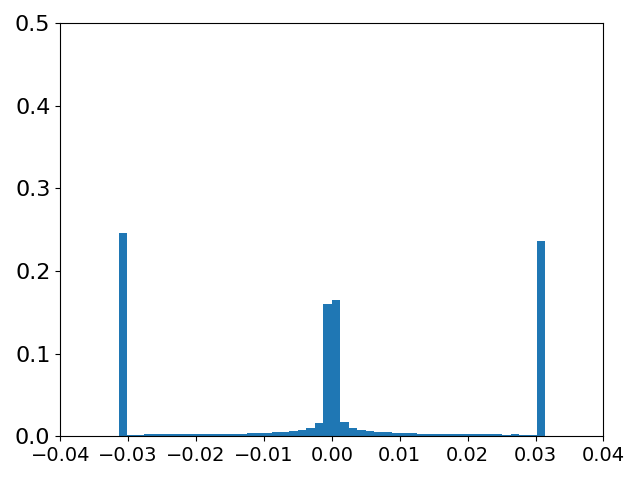
PGD Coefficient Histogram
PGD (raw) Coefficient Histogram
RGD Coefficient Histogram
\stackunder[5pt] step1
\stackunder[5pt]
step1
\stackunder[5pt] step3
\stackunder[5pt]
step3
\stackunder[5pt] step5
\stackunder[5pt]
step5
\stackunder[5pt] step7
step7


4.1 Theoretical Insights
In this part, we characterize the influence of the update procedure on the adversarial gain at each step . Inspired by existing works (Du et al., 2019; Arora et al., 2019), we consider a model function with one ReLU (Nair and Hinton, 2010) hidden layer, defined as follows:
| (4) |
where denotes the element-wisely ReLU function, denotes the input, and denote output weight and first-layer vector weight respectively. Assuming the Mean Square Error (MSE) loss, the loss function is defined as follows:
| (5) |
where denotes the real label value for input .
Theorem 1.
Considering , activation function as ReLU, we define as element wise absolute operation, then the adversarial step gain is bounded as follows:
where denotes the clipped perturbation in -th step.
The theorem demonstrates that the adversarial gain in step depends on two factors: (i) The magnitude of perturbation change, . If the update algorithm results in a large perturbation change, the adversarial gain will be increased. (ii) The previous adversarial loss , and the updated loss . It is important to note that the adversarial loss is non-negative, and we expect the updated to be greater than the previous . Therefore, the step gain is highly influenced by the previous loss . As a result, a larger previous adversarial loss implies a better step gain. In summary, if our update algorithm induces a significant perturbation change and starts with a substantial initial adversarial loss , it will lead to a larger adversarial gain .
| Dataset | Method | PGD | PGD(raw) | RGD |
| CIFAR-10 () | WRN-28(Ding et al., 2020) | 52.64 | 53.98 | 52.56 |
| PreRN-18(Wong et al., 2020) | 47.45 | 47.50 | 47.31 | |
| RN-18(Addepalli et al., 2022) | 57.06 | 57.11 | 57.03 | |
| RN-18(Engstrom et al., 2019) | 43.23 | 44.50 | 42.87 | |
| CIFAR-10 () | WRN-28(Ding et al., 2020) | 37.53 | 40.93 | 37.19 |
| PreRN-18(Wong et al., 2020) | 13.32 | 14.98 | 12.99 | |
| RN-18(Addepalli et al., 2022) | 25.57 | 25.87 | 25.27 | |
| RN-18(Engstrom et al., 2019) | 14.19 | 19.11 | 13.37 | |
| CIFAR-100 () | WRN-28(Wang et al., 2023) | 21.10 | 20.72 | 20.61 |
| XCiT(Debenedetti et al., 2022) | 15.28 | 15.44 | 15.28 | |
| WRN-34(Addepalli et al., 2022) | 16.37 | 16.16 | 15.94 | |
| RN-18(Addepalli et al., 2022) | 14.45 | 14.40 | 14.20 | |
| PreRN-18(Rice et al., 2020) | 6.14 | 7.36 | 5.78 | |
| ImageNet () | WRN-50(Salman et al., 2020) | 42.02 | 42.57 | 41.88 |
| RN-50(Wong et al., 2020) | 29.0 | 28.56 | 27.85 | |
| RN-18(Salman et al., 2020) | 30.08 | 30.45 | 30.08 | |
| ImageNet () | WRN-50(Salman et al., 2020) | 19.35 | 21.75 | 18.97 |
| RN-50(Wong et al., 2020) | 11.77 | 12.31 | 11.03 | |
| RN-18(Salman et al., 2020) | 12.88 | 13.69 | 12.68 | |
4.2 Empirical Study
We next conduct a further study to analyze how the update process shapes adversarial samples in practice. Specifically, we target the robust PGD model 111The robust model used can be found at https://github.com/ndb796/Pytorch-Adversarial-Training-CIFAR with CIFAR10 setting. on the CIFAR10 testing dataset within the ball. The perturbation distribution at each step for three update algorithms (PGD, PGD with raw update, proposed RGD) is illustrated in Figure 1. The results reveal that, within the limited 7 steps, the majority of pixels (86.9%) converge to the boundary in the PGD update, whereas its corresponding raw update shows a lower boundary ratio (59.1%) with a considerable number of pixels remaining stuck at the zero initial point. More detailed information regarding the boundary ratio and robust accuracy can be found in Table 1. It reveals that PGD achieves a lower robust accuracy () compared to its raw update version (). Considering the theoretical results presented in Theorem 1, which indicate that larger perturbation changes lead to better performance gains, we can conclude that the success of PGD, in contrast to PGD with naive raw update, can be attributed to its "sign" ability, which facilitates more pixel changes and convergence to the boundary.
Furthermore, it is worth noting that RGD outperforms PGD in terms of attack performance, despite having fewer boundary pixels (70.6% v.s. 86.9%). This can be attributed to the fact that the real adversarial distribution in RGD exhibits better attack performance, as indicated by the higher values of , resulting in larger adversarial gains at each step, as demonstrated in Table 1. Consequently, RGD is able to learn a better adversarial distribution even without a significant perturbation change. It is important to highlight that PGD (raw), despite its use of raw updates, does not effectively preserve most of the magnitude information due to the clip operation. As a result, it performs significantly worse than RGD.
To ensure a fair comparison, we carefully fine-tuned the step size for all three algorithms, using grid search. Following the principle of minimal robust accuracy, we set a zero initial point for both PGD (raw) and RGD, while utilizing a random initial point for PGD. Note that the choice of initial point does not influence the final boundary ratio while detailed initial comparison is available in Appendix B.
5 Experimental Results
In this section, we begin by comparing the proposed RGD algorithm with PGD (sign/raw updates) for adversarial attacks on different architectures, with varying adversarial perturbation levels and datasets. Then we compare RGD and PGD over adversarial training setting and showcase the robust accuracy performance boosts brought by RGD. Moreover, we utilize RGD for transfer attacks and conduct extensive experiments to validate its remarkable improvement in adversarial transferability. All experiments are conducted with five independent runs with different random seeds, and the standard deviations are reported to affirm results’ significance. The step sizes for all algorithms are carefully tuned through grid search. For the PGD, we grid search the step size from list (2, 1.5, , 0.8, 0.5, 0.25, 0.2) and our RGD, PGD(raw) step size tuned from list (1, 3, 10, 30, 100, 300, 1000, 3000, 1e4, 3e4, etc). The step size for RGD and PGD(raw) is larger than PGD ones because the raw gradient over the input is small which calls for a large step size for update. Meanwhile, we utilize random initialization for PGD and zero initialization for the other methods. The initial choice is based on minimal robust accuracy principle. The detailed initial comparison is available in Appendix B. All experiments use NVIDIA Volta V100 GPUs.
5.1 Comparison of Algorithms for Adversarial Attack
We compare PGD with sign/raw updates and proposed RGD using a 7-step attack. The datasets include CIFAR-10, CIFAR-100, and ImageNet, and we attack their respective testing or validation sets. The models attacked are sourced from RobustBench (Croce et al., 2021). The adversarial attack settings follows the approach of Ding et al. (2019), and the results are presented in Table 2.
Our results demonstrate that introduced non-clipped perturbation significantly improves the raw update method, resulting in a substantial performance boost from PGD (raw) to RGD. Furthermore, RGD outperforms PGD across various datasets, model architectures, and adversarial sizes, highlighting the superiority of RGD. It is worth noting that RGD is particularly advantageous in scenarios with larger values (e.g., ). This is likely because larger adversarial size allows RGD to exhibit a more effective adversarial distribution. Conversely, if a smaller -ball is used, most RGD perturbation pixels will be clipped into the boundary in the final step.
5.2 Comparison of Algorithms for Adversarial Training
For adversarial training, we conduct experiments with different architectures and steps on CIFAR10 to compare PGD and RGD. We specifically train models including ResNet, WideResNet, and a Convolutional Neural Network, using both 5-step and 10-step attack strategies. Each model comprises 6 blocks. The robustness of these models is assessed using a 10-step Projected Gradient Descent (PGD) attack, with all experiments conducted within an constraint. Both clean and robust accuracy results are presented in Table 3.
| Setting | Method | Clean Accuracy | Robust Accuracy |
| ResNet (Step=5) | PGD | 84.41 % | 29.32 % |
| RGD | 76.35% | 44.67% (15.35%) | |
| ResNet (Step=10) | PGD | 79.41% | 38.15 % |
| RGD | 78.35% | 47.16% (9.01%) | |
| WideResNet (Step=5) | PGD | 89.83% | 37.86 % |
| RGD | 86.17% | 52.15% (14.29%) | |
| WideResNet (Step=10) | PGD | 80.53% | 48.33 % |
| RGD | 86.04% | 52.19% (3.86%) | |
| CNN (Step=5) | PGD | 86.85% | 26.00 % |
| RGD | 82.72% | 42.76% (16.76%) | |
| CNN (Step=10) | PGD | 82.10% | 41.35 % |
| RGD | 82.63% | 43.03% (1.68%) | |
From the table, it can be observed that RGD significantly improves all robust accuracy across different architectures and steps. Specifically, for the setting of WideResNet step=10, RGD improves both clean and robust accuracy. For the other settings of CNN step=5, RGD sacrifices a little clean accuracy of but significantly improves the robust accuracy of than PGD. All these experimental results further validate the superiority of RGD over PGD, especially with setting of step=5.
| Dataset | Method | Type | PGD | PGD (raw) | RGD |
| ImageNet () | ResNet-50 | Source | 99.97 | 96.73 | 99.30 |
| DenseNet-121 | Clean | 54.52 | 24.34 | 59.42 | |
| VGG19-BN | Clean | 51.06 | 26.51 | 59.40 | |
| Inception-V3 | Clean | 29.04 | 22.42 | 34.82 | |
| PreActResNet-18 | Robust | 30.09 | 30.51 | 30.88 | |
| WideResNet-50 | Robust | 12.13 | 12.55 | 12.77 | |
| ResNet-50 | Robust | 18.14 | 18.81 | 19.11 | |
| ImageNet () | ResNet-50 | Source | 100 | 98.08 | 99.30 |
| DenseNet-121 | Clean | 77.58 | 42.76 | 81.1 | |
| VGG19-BN | Clean | 72.67 | 49.98 | 80.62 | |
| Inception-V3 | Clean | 44.04 | 35.01 | 54.6 | |
| PreActResNet-18 | Robust | 34 | 37.66 | 38.22 | |
| WideResNet-50 | Robust | 15.03 | 19.12 | 19.62 | |
| ResNet-50 | Robust | 21.96 | 26.81 | 27.52 | |
| CIFAR-10 () | ResNet-50 | Source | 98.76 | 78.99 | 98.22 |
| DenseNet-121 | Clean | 65.74 | 43.05 | 79.66 | |
| VGG19-BN | Clean | 58.20 | 45.87 | 72.23 | |
| Inception-V3 | Clean | 64.28 | 49.87 | 77.3 | |
| WideResNet-28 | Robust | 17.41 | 17.86 | 18.88 | |
| PreActResNet-181 | Robust | 18.11 | 18.06 | 19.01 | |
| PreActResNet-182 | Robust | 21.46 | 21.62 | 22.54 | |
| CIFAR-10 () | ResNet50 | Source | 99.9 | 90.32 | 99.22 |
| DenseNet-121 | Clean | 89.36 | 76.5 | 95.51 | |
| VGG19-BN | Clean | 82.90 | 79.17 | 90.8 | |
| Inception-V3 | Clean | 86.61 | 79.7 | 93.49 | |
| WideResNet-28 | Robust | 19.9 | 22.42 | 23.90 | |
| PreActResNet-181 | Robust | 19.98 | 21.67 | 23.53 | |
| PreActResNet-182 | Robust | 23.23 | 24.49 | 26.03 | |


5.3 Transfer Attack Study
In this section, we examine and compare the transferability of RGD with PGD (sign/raw). We begin by generating adversarial data through a 10-step attack on the clean ResNet50 model (He et al., 2016). These adversarial samples are then transferred to attack clean (Simonyan and Zisserman, 2015; Huang et al., 2017; Szegedy et al., 2015) and robust (Croce et al., 2021) target models. The ImageNet validation set and CIFAR-10 testing set are used as the data for the attacks, following the settings in Zhao et al. (2022). The detailed results of the attack success rates for the source and target models can be found in Table 4.
The findings demonstrate that RGD consistently achieves the highest target success rates, while maintaining similar source success rates compared to PGD. It consistently improves the success rate by at least 5% when attacking most clean models and by around 3% for robust models with larger boundary (). Furthermore, PGD (raw) outperforms signed PGD when attacking robust models, indicating that raw updates enhance the transferability to robust models. Our proposed RGD method further improves both robust and clean transferability compared to PGD (raw).
6 Ablation and Visualization
6.1 Adversarial Perturbation Level Study
In this section, we conduct a comprehensive comparison under different levels of adversarial perturbation. Specifically, we consider three different values of () for generating adversarial examples, and evaluate the robust accuracy of PGD with sign or raw gradient updates, as well as RGD, when attacking the robust ResNet18 model using the same settings as in Section 4.2. We perform a grid search to determine the step sizes for each algorithm, and the results are presented in Figure 2, where a lower robust accuracy indicates a stronger attack.
Our result reveals the following observations: In the context of small (), all algorithms converge to a similar performance point, suggesting comparable attack effectiveness. However, for larger size (), PGD with raw gradient update performs relatively poorly, while RGD outperforms the other algorithms with noticeable improvements. Therefore, when a larger perturbation is allowed, RGD is the preferred choice for achieving stronger attack performance.
Furthermore, the raw update-based algorithms, namely PGD (raw) and RGD, exhibit a lower robust accuracy in the early steps. It is important to mention that we utilize zero initial for PGD (raw) and RGD, while a stronger uniform random initialization for PGD. This suggests that the raw update enables the generation of high-quality adversarial examples in the early steps.
6.2 Adversarial Update Step Study
In this section, we compare the performance of PGD with sign/raw updates and RGD at different update steps. Specifically, we evaluate the algorithms at steps 5, 10 and 20. The experimental setup follows Section 4.2 where step sizes are carefully fine-tuned. We fix the adversarial size at , and the results are presented in Figure 3.
Our findings reveal that in the early stages, RGD achieves a lower robust accuracy compared to PGD, which can be attributed to its generation of stronger adversarial examples through a genuine adversarial distribution. However, as the number of training steps increases, the performance gap between RGD and PGD diminishes. This can be explained by the stable perturbation change introduced by the sign function in PGD, allowing it to achieve comparable performance to RGD in the later steps. In summary, RGD is a preferable choice for scenarios requiring a few-step update.
Additionally, it is evident that PGD with raw update remains in a suboptimal performance region and shows limited improvement in the later steps. This observation further highlights the advantage of the non-clipping design in RGD, which facilitates the generation of stronger adversarial examples.
7 Conclusion
This work provides a theoretical analysis of how update procedures impact adversarial performance and offers an empirical explanation for why the sign operation is preferred in PGD. Additionally, we introduce the hidden unclipped perturbation and propose a novel attack algorithm called RGD. This algorithm transforms the constrained optimization problem into an unconstrained optimization problem. Extensive experiments have been conducted to demonstrate the superiority of proposed algorithm in practical scenarios.
References
- Addepalli et al. (2022) S. Addepalli, S. Jain, et al. Efficient and effective augmentation strategy for adversarial training. Advances in Neural Information Processing Systems (NeurIPS), 35:1488–1501, 2022.
- Agarwal et al. (2020) A. Agarwal, R. Singh, and M. Vatsa. The role of’sign’and’direction’of gradient on the performance of cnn. In Proceedings of the IEEE/CVF Conference on Computer Vision and Pattern Recognition Workshops, pages 646–647, 2020.
- Al-Dujaili and O’Reilly (2020) A. Al-Dujaili and U.-M. O’Reilly. Sign bits are all you need for black-box attacks. In International Conference on Learning Representations, 2020.
- Andriushchenko and Flammarion (2020) M. Andriushchenko and N. Flammarion. Understanding and improving fast adversarial training. Advances in Neural Information Processing Systems (NeurIPS), 33:16048–16059, 2020.
- Andriushchenko et al. (2020) M. Andriushchenko, F. Croce, N. Flammarion, and M. Hein. Square attack: a query-efficient black-box adversarial attack via random search. In European Conference on Computer Vision (ECCV), pages 484–501. Springer, 2020.
- Arora et al. (2019) S. Arora, S. Du, W. Hu, Z. Li, and R. Wang. Fine-grained analysis of optimization and generalization for overparameterized two-layer neural networks. In International Conference on Machine Learning (ICML), pages 322–332, 2019.
- Carlini and Wagner (2017) N. Carlini and D. Wagner. Towards evaluating the robustness of neural networks. In 2017 ieee symposium on security and privacy (sp), pages 39–57. Ieee, 2017.
- Chen and Gu (2020) J. Chen and Q. Gu. Rays: A ray searching method for hard-label adversarial attack. In Proceedings of the 26th ACM SIGKDD International Conference on Knowledge Discovery & Data Mining (KDD), pages 1739–1747, 2020.
- Chen et al. (2017) P.-Y. Chen, H. Zhang, Y. Sharma, J. Yi, and C.-J. Hsieh. Zoo: Zeroth order optimization based black-box attacks to deep neural networks without training substitute models. In Proceedings of the 10th ACM workshop on artificial intelligence and security, pages 15–26, 2017.
- Croce and Hein (2020) F. Croce and M. Hein. Reliable evaluation of adversarial robustness with an ensemble of diverse parameter-free attacks. In International Conference on Machine Learning (ICML), pages 2206–2216. PMLR, 2020.
- Croce et al. (2021) F. Croce, M. Andriushchenko, V. Sehwag, E. Debenedetti, N. Flammarion, M. Chiang, P. Mittal, and M. Hein. Robustbench: a standardized adversarial robustness benchmark. In Thirty-fifth Conference on Neural Information Processing Systems Datasets and Benchmarks Track, 2021. URL https://openreview.net/forum?id=SSKZPJCt7B.
- Debenedetti et al. (2022) E. Debenedetti, V. Sehwag, and P. Mittal. A light recipe to train robust vision transformers. arXiv preprint arXiv:2209.07399, 2022.
- Ding et al. (2019) G. W. Ding, L. Wang, and X. Jin. AdverTorch v0.1: An adversarial robustness toolbox based on pytorch. arXiv preprint arXiv:1902.07623, 2019.
- Ding et al. (2020) G. W. Ding, Y. Sharma, K. Y. C. Lui, and R. Huang. Mma training: Direct input space margin maximization through adversarial training. In International Conference on Learning Representations (ICLR), 2020.
- Dong et al. (2018) Y. Dong, F. Liao, T. Pang, H. Su, J. Zhu, X. Hu, and J. Li. Boosting adversarial attacks with momentum. In Proceedings of the IEEE conference on computer vision and pattern recognition, pages 9185–9193, 2018.
- Du et al. (2019) S. S. Du, X. Zhai, B. Poczos, and A. Singh. Gradient descent provably optimizes over-parameterized neural networks. In International Conference on Learning Representations (ICLR), 2019.
- Engstrom et al. (2019) L. Engstrom, A. Ilyas, H. Salman, S. Santurkar, and D. Tsipras. Robustness (python library), 2019. URL https://github.com/MadryLab/robustness.
- Goodfellow et al. (2015) I. J. Goodfellow, J. Shlens, and C. Szegedy. Explaining and harnessing adversarial examples. In International Conference on Learning Representations (ICLR), 2015.
- He et al. (2016) K. He, X. Zhang, S. Ren, and J. Sun. Deep residual learning for image recognition. In Proceedings of the IEEE conference on computer vision and pattern recognition (CVPR), pages 770–778, 2016.
- Hochreiter and Schmidhuber (1997) S. Hochreiter and J. Schmidhuber. Long short-term memory. Neural computation, 9(8):1735–1780, 1997.
- Huang et al. (2017) G. Huang, Z. Liu, L. Van Der Maaten, and K. Q. Weinberger. Densely connected convolutional networks. In Proceedings of the IEEE conference on computer vision and pattern recognition (CVPR), pages 4700–4708, 2017.
- Huang et al. (2021) H. Huang, Y. Wang, S. Erfani, Q. Gu, J. Bailey, and X. Ma. Exploring architectural ingredients of adversarially robust deep neural networks. Advances in Neural Information Processing Systems (NeurIPS), 34:5545–5559, 2021.
- Ilyas et al. (2018) A. Ilyas, L. Engstrom, A. Athalye, and J. Lin. Black-box adversarial attacks with limited queries and information. In International conference on machine learning, pages 2137–2146. PMLR, 2018.
- Jia et al. (2022) X. Jia, Y. Zhang, B. Wu, K. Ma, J. Wang, and X. Cao. Las-at: adversarial training with learnable attack strategy. In Proceedings of the IEEE/CVF Conference on Computer Vision and Pattern Recognition (CVPR), pages 13398–13408, 2022.
- Krizhevsky et al. (2012) A. Krizhevsky, I. Sutskever, and G. E. Hinton. Imagenet classification with deep convolutional neural networks. In F. Pereira, C. Burges, L. Bottou, and K. Weinberger, editors, Advances in Neural Information Processing Systems (NeurIPS), volume 25. Curran Associates, Inc., 2012.
- Kurakin et al. (2018) A. Kurakin, I. J. Goodfellow, and S. Bengio. Adversarial examples in the physical world. In Artificial intelligence safety and security, pages 99–112. Chapman and Hall/CRC, 2018.
- Liu et al. (2019) S. Liu, P.-Y. Chen, X. Chen, and M. Hong. signsgd via zeroth-order oracle. In International conference on learning representations. International Conference on Learning Representations (ICLR), 2019.
- Madry et al. (2018) A. Madry, A. Makelov, L. Schmidt, D. Tsipras, and A. Vladu. Towards deep learning models resistant to adversarial attacks. In International Conference on Learning Representations (ICLR), 2018.
- Moosavi-Dezfooli et al. (2016) S.-M. Moosavi-Dezfooli, A. Fawzi, and P. Frossard. Deepfool: a simple and accurate method to fool deep neural networks. In Proceedings of the IEEE conference on computer vision and pattern recognition (CVPR), pages 2574–2582, 2016.
- Nair and Hinton (2010) V. Nair and G. E. Hinton. Rectified linear units improve restricted boltzmann machines. In Proceedings of the 27th international conference on machine learning (ICML), 2010.
- Rebuffi et al. (2021) S.-A. Rebuffi, S. Gowal, D. A. Calian, F. Stimberg, O. Wiles, and T. Mann. Fixing data augmentation to improve adversarial robustness. arXiv preprint arXiv:2103.01946, 2021.
- Rice et al. (2020) L. Rice, E. Wong, and Z. Kolter. Overfitting in adversarially robust deep learning. In International Conference on Machine Learning (ICML), pages 8093–8104, 2020.
- Salman et al. (2020) H. Salman, A. Ilyas, L. Engstrom, A. Kapoor, and A. Madry. Do adversarially robust imagenet models transfer better? Advances in Neural Information Processing Systems (NeurIPS), 33:3533–3545, 2020.
- Shaham et al. (2015) U. Shaham, Y. Yamada, and S. Negahban. Understanding adversarial training: Increasing local stability of neural nets through robust optimization. arXiv preprint arXiv:1511.05432, 2015.
- Simonyan and Zisserman (2015) K. Simonyan and A. Zisserman. Very deep convolutional networks for large-scale image recognition. In International Conference on Learning Representations (ICLR), 2015.
- Szegedy et al. (2013) C. Szegedy, W. Zaremba, I. Sutskever, J. Bruna, D. Erhan, I. Goodfellow, and R. Fergus. Intriguing properties of neural networks. arXiv preprint arXiv:1312.6199, 2013.
- Szegedy et al. (2015) C. Szegedy, W. Liu, Y. Jia, P. Sermanet, S. Reed, D. Anguelov, D. Erhan, V. Vanhoucke, and A. Rabinovich. Going deeper with convolutions. In Proceedings of the IEEE conference on computer vision and pattern recognition (CVPR), pages 1–9, 2015.
- Wang et al. (2023) Z. Wang, T. Pang, C. Du, M. Lin, W. Liu, and S. Yan. Better diffusion models further improve adversarial training. arXiv preprint arXiv:2302.04638, 2023.
- Wong et al. (2020) E. Wong, L. Rice, and J. Z. Kolter. Fast is better than free: Revisiting adversarial training. In International Conference on Learning Representations (ICLR), 2020.
- Wu et al. (2020) D. Wu, S.-T. Xia, and Y. Wang. Adversarial weight perturbation helps robust generalization. Advances in Neural Information Processing Systems (NeurIPS), 33:2958–2969, 2020.
- Zhang et al. (2020) J. Zhang, J. Zhu, G. Niu, B. Han, M. Sugiyama, and M. Kankanhalli. Geometry-aware instance-reweighted adversarial training. arXiv preprint arXiv:2010.01736, 2020.
- Zhang et al. (2021) Y. Zhang, M. Gong, T. Liu, G. Niu, X. Tian, B. Han, B. Schölkopf, and K. Zhang. Causaladv: Adversarial robustness through the lens of causality. arXiv preprint arXiv:2106.06196, 2021.
- Zhang et al. (2022) Y. Zhang, G. Zhang, P. Khanduri, M. Hong, S. Chang, and S. Liu. Revisiting and advancing fast adversarial training through the lens of bi-level optimization. In International Conference on Machine Learning (ICML), pages 26693–26712. PMLR, 2022.
- Zhao et al. (2022) Z. Zhao, H. Zhang, R. Li, R. Sicre, L. Amsaleg, and M. Backes. Towards good practices in evaluating transfer adversarial attacks. arXiv preprint arXiv:2211.09565, 2022.
Supplementary Materials
Appendix A Comparison with AutoAttack
AutoAttack (Croce and Hein, 2020) is an ensemble adversarial algorithm known for its success in adversarial attacks. One of its components, APGDCE, is a variant of the PGD algorithm. The results from Section 4.2 and 6.2 demonstrate that RGD is capable of learning the genuine adversarial distribution, resulting in stronger attack in the early steps. In contrast, PGD benefits from the larger perturbation changes introduced by the sign function, which leads to great performance in the later steps. Therefore, we integrate RGD into the 100-step APGDCE algorithm by replacing the first two APGD updates with RGD updates. Specifically, we implement APGDCE+RGD without restarting, and RGD is initialized with zero values. The step size for RGD is carefully fine-tuned based on the first two step performance. The selection of two steps was motivated by its ability to yield the most significant enhancements in most scenarios. A comprehensive comparison of the improvements observed in the initial two steps is available in Appendix D. Following the same experimental setup in Croce and Hein (2020), we present comparison between APGDCE and APGDCE+RGD for their final robust accuracy in Table 5.
| Dataset | Method | APGDCE | APGDCE+RGD |
| CIFAR-10 () | WRN-34(Huang et al., 2021) | 23.48 | 23.35 |
| WRN-28(Wu et al., 2020) | 28.0 | 27.81 | |
| PreRN-18(Wong et al., 2020) | 9.63 | 9.58 | |
| CIFAR-100 () | WRN-28(Wang et al., 2023) | 19.43 | 19.31 |
| WRN-70(Rebuffi et al., 2021) | 16.88 | 16.55 | |
| XCiT(Debenedetti et al., 2022) | 13.77 | 13.71 | |
| WRN-34(Jia et al., 2022) | 11.56 | 11.28 | |
| ImageNet () | RN-18(Salman et al., 2020) | 29.32 | 29.26 |
| XCiT(Debenedetti et al., 2022) | 42.73 | 42.73 | |
| PreRN-18(Wong et al., 2020) | 27.18 | 27.07 | |
| WRN-50(Salman et al., 2020) | 40.86 | 40.76 | |
Our results demonstrate that despite the initial disadvantage of zero initialization, RGD achieves a lower robust accuracy compared to APGD in the first two steps as shown in Appendix D, highlighting its superiority. Furthermore, RGD maintains this advantage in the final stage across most scenarios as shown in Table 5. It is worth noting that such considerable performance improvement is achieved by only modifying the first two steps out of the 100 updates.
Appendix B Comparison of Initials
For initialization, we choose methods based on their suitability: PGD favors random initialization, while RGD and PGD (raw) lean towards zero initialization. To illustrate, we present the robust accuracy outcomes when attacking the robust ResNet18 model using various initial values:
| Method | Random Initial | Zero Initial |
| PGD | 43.2% | 43.27% |
| PGD (raw) | 44.65% | 44.49% |
| RGD | 42.91% | 42.88% |
From Table 6, it is evident that PGD benefits from random initialization, whereas PGD (raw) and RGD perform better with zero initialization. Moreover, RGD exhibits superior performance in both contexts.
Appendix C Pixel-wise Experiments
To better illustrate that PGD enjoys larger perturbation change per step compared with RGD, we calculate the average pixel-wise perturbation change when attacking the robust ResNet18 model. The results are shown below:
| Algorithm | 1 | 2 | 3 | 4 | 5 | 6 | 7 | |
| Perturbation change | PGD | 0.0167 | 0.0119 | 0.0077 | 0.005 | 0.0041 | 0.0035 | 0.0032 |
| PGD (raw) | 0.0116 | 0.0082 | 0.006 | 0.0054 | 0.0049 | 0.0048 | 0.0048 | |
| RGD | 0.0146 | 0.0084 | 0.0048 | 0.003 | 0.0022 | 0.0019 | 0.0017 | |
From Table 7, it is evident that RGD undergoes smaller perturbation shifts than PGD, leading to a decreased boundary ratio as depicted in Table 1. Despite these minor perturbation variations, RGD, benefiting from genuine adversarial perturbations, surpasses PGD in performance. However, the edge of this improvement narrows with increasing iterations.
In the case of PGD (raw), while it might show pronounced perturbation changes in later stages, its adversarial loss remains suboptimal, and it lacks consistent convergence stability. As a result, when compared to both PGD and RGD, performance of PGD (raw) is notably inferior.
Appendix D AutoAttack Extra Experimental Results
| Dataset | Method | APGDCE | APGDCE+RGD |
| CIFAR10 () | WRN-34(Huang et al., 2021) | 90.0147.73 | 91.2345.79 |
| WRN-28(Wu et al., 2020) | 86.4641.71 | 88.2539.3 | |
| PreRN-18(Wong et al., 2020) | 81.8524.75 | 83.3421.72 | |
| CIFAR100 () | WRN-28(Wang et al., 2023) | 70.7225.6 | 72.5824.17 |
| WRN-70(Rebuffi et al., 2021) | 61.7322.75 | 63.5621.44 | |
| XCiT(Debenedetti et al., 2022) | 65.6419.88 | 67.3419.16 | |
| WRN-34(Jia et al., 2022) | 65.1121.44 | 67.3120.33 | |
| ImageNet () | RN-18(Salman et al., 2020) | 52.6431.28 | 52.8830.68 |
| XCiT(Debenedetti et al., 2022) | 72.0446.58 | 72.0645.72 | |
| PreRN-18(Wong et al., 2020) | 52.9730.94 | 53.4630.12 | |
| WRN-50(Salman et al., 2020) | 68.3644.96 | 68.6243.9 | |
In this section, we evaluate the improvement in the first two steps of accuracy for APGD and APGD+RGD. The results are shown in Table 8. We can observe that despite having a worse initialization (zero initialization), RGD achieves a lower robust accuracy after two steps compared to APGD, indicating its superiority. Furthermore, APGD+RGD maintains these advantages in the final accuracy, as demonstrated in Table 5.
Appendix E Related Lemmas
Lemma 1.
Considering activation function as ReLU, i.e., , then we define as element wise absolute operation, and obtain
where follows because , follows because , follows because all elements in are non-negative, all elements in are non-positive and follows because . Then, we take absolute operation for both sides and obtain:
where is defined as element wise absolute operation.
Lemma 2.
Considering , then we obtain
where follows from definition.