Rethinking binary hyperparameters for deep transfer learning for image classification
Abstract
The current standard for a variety of computer vision tasks using smaller numbers of labelled training examples is to fine-tune from weights pre-trained on a large image classification dataset such as ImageNet. The application of transfer learning and transfer learning methods tends to be rigidly binary. A model is either pre-trained or not pre-trained. Pre-training a model either increases performance or decreases it, the latter being defined as negative transfer. Application of L2-SP regularisation that decays the weights towards their pre-trained values is either applied or all weights are decayed towards 0. This paper re-examines these assumptions. Our recommendations are based on extensive empirical evaluation that demonstrate the application of a non-binary approach to achieve optimal results. (1) Achieving best performance on each individual dataset requires careful adjustment of various transfer learning hyperparameters not usually considered, including number of layers to transfer, different learning rates for different layers and different combinations of L2SP and L2 regularization. (2) Best practice can be achieved using a number of measures of how well the pre-trained weights fit the target dataset to guide optimal hyperparameters. We present methods for non-binary transfer learning including combining L2SP and L2 regularization and performing non-traditional fine-tuning hyperparameter searches. Finally we suggest heuristics for determining the optimal transfer learning hyperparameters. The benefits of using a non-binary approach are supported by final results that come close to or exceed state of the art performance on a variety of tasks that have traditionally been more difficult for transfer learning.
1 Introduction
Convolutional neural networks (CNNs) have achieved many successes in image classification in recent years [17, 9, 19, 24, 25]. It has been consistently demonstrated that CNNs work best when there is abundant labelled data available for the task and very deep models can be trained [28, 22, 14]. However, there are many real world scenarios where the large amounts of training data required to obtain the best performance cannot be met or are prohibitively expensive. Transfer learning has been shown to improve performance in a wide variety of computer vision tasks, particularly when the source and target tasks are closely related and the target task is small [28, 22, 6, 8, 33, 27, 21, 20, 37]. It has become standard practice to pre-train on Imagenet 1K for many different tasks where the available labeled datasets are orders of magnitude smaller than Imagenet 1K [21, 20, 37, 24, 19, 27, 25, 26, 9]. Several papers published in recent years have questioned this established paradigm. They have shown that when the target dataset is very different from Imagenet 1K and a reasonable amount of data is available, training from scratch can match or even out perform pre-trained and fine-tuned models [12, 35, 34, 40, 22].
The standard transfer learning strategy is to transfer all layers apart from the final classification layer, and either use a single initial learning rate and other hyperparameters for fine-tuning all layers, or freeze some layers. Given that lower layers in a deep neural network are known to be more general and higher layers more specialised [39], we argue that the binary way of approaching transfer learning and fine-tuning is counter intuitive. There is no intuitive reason to think that all layers should be treated the same when fine-tuning, or that pre-trained weights from all layers will be applicable to the new task. If transferring all layers results in negative transfer, could transferring some number of lower more general layers improve performance? If using an L2SP weight decay on all transferred layers for regularisation decreases performance over decaying towards 0, might applying the L2SP regularisation to some number of lower layers that are more applicable to the target dataset result in improved performance?
We performed extensive experiments across four different datasets to:
-
•
re-examine the assumptions that transfer learning hyperparameters should be binary, and
-
•
find the optimal settings for number of layers to transfer, initial learning rates for different layers, and number of layers to apply L2SP regularisation vs decaying towards 0.
We developed methods for non-binary transfer learning including combining L2SP and L2 regularization and performing non-traditional fine-tuning hyperparameter searches. We show that the optimal settings result in significantly better performance than binary settings for all datasets except the most closely related. Finally we suggest heuristics for determining the optimal transfer learning hyperparameters.
2 Related work
The standard transfer learning strategy is to transfer all layers apart from the final classification layer, then use a search strategy to find the best single initial learning rate and other hyperparameters. Several studies include extensive hyperparameter searches over learning rate and weight decay [15, 22], momentum [18], and L2SP [21]. This commonly used strategy originates from various works showing that performance on the target task increases as the number of layers transferred increases [39, 4, 1, 2]. All these works were completed prior to advances in residual networks [13], and other advances to improve learning for deep CNN architectures, and searches for optimal combinations of learning rates and number of layers to transfer were not performed. Additionally, in two of the works layers that were not transferred were discarded completely rather than reinitialising and training them from scratch. This resulted in smaller models with less layers transferred and a strong bias towards better results when more layers were transferred [1, 2]. Further studies have shown the combination of a lower learning rate and fewer layers transferred may be optimal [30]. However, again modern residual networks were not used and only very similar source and target datasets were selected.
It has been shown that the similarity between source and target datasets has a strong impact on performance for transfer learning:
- 1.
-
2.
A multi-step pre-training process where the interim dataset is smaller and more closely related to the target dataset can outperform a single step pre-training process when originating from a very different, large source dataset [27].
-
3.
Self-supervised pre-training on a closely related source dataset can be better than supervised training on a less closely related dataset [42].
- 4.
-
5.
Momentum should be lower for more closely related source and target datasets [18].
These five factors demonstrate the importance of the relationship between the source and target dataset in transfer learning.
3 Methodology
3.1 Datasets
We performed evaluations on four different small target datasets, each being less than 10,000 training images. We chose one that is very similar to Imagenet 1K that transfer learning and sub methods have traditionally performed best on. This is used as a baseline for comparison to show that the default methods that perform badly on the other datasets chosen do perform well on this one. For each of the other target datasets it has been shown that traditional transfer learning strategies:
-
•
do not perform well on them and/or
-
•
they are very different to the source dataset used for pre-training.
We used the standard available train, validation and test splits for the three datasets for which they were available. For Caltech256-30 we used the first 30 items from each class for the train split, the next 20 for the validation split and the remainder for the test split.
3.1.1 Source dataset
We used Imagenet 1K as the source dataset as it is most commonly used source dataset and therefore the most suitable to demonstrate our approach.
3.1.2 Target datasets
These are the final datasets that we transferred the models to and measured performance on. We used a standard 299 299 image size for all datasets.
Most similar to Imagenet 1K
We chose Caltech 256-30 (Caltech) [10] as the most similar to Imagenet. It contains 256 different general subordinate and superordinate classes. As our focus is on small target datasets, we chose the smallest commonly used split with 30 examples per class.
Fine-grained
Very different to Imagenet 1K
We evaluated performance on another dataset that is intuitively very different to Imagenet 1K as it consists of images depicting adjectives instead of nouns.
-
•
Describable Textures (DTD) [5]: consists of 3,760 training examples of texture images jointly annotated with 47 attributes. The texture images are collected “in the wild” by searching for texture adjectives on the web.
3.2 Model
Inception v4 [36] was selected for evaluation as it has been shown to have state of the art performance for transferring from Imagenet 1K to a broad range of target tasks [15]. Our code is adapted from [38] and we used the publicly available pre-trained Inception v4 model. Our code is available at https://anonymous.4open.science/r/Non-binary-deep-transfer-learning-for-image-classification-872D. We did not experiment with pre-training settings, for example removing regularization settings as suggested by [15], as it was beyond the scope of this work and the capacity of our compute resources.
3.3 Evaluation metric
We used top-1 accuracy for all results for easiest comparison with existing results on the chosen datasets. Graphs showing ablation studies with different hyperparameters show results on one run. Final reported results are averages and standard deviations over four runs. For all experiments we used single crop and for our final comparison to state of the art for each dataset we used an ensemble of all four runs and 10-crop.
3.4 Compute resources
The experiments were run on compute nodes containing four Nvidia V100 GPUs and two 24-core Intel Xeon Scalable ’Cascade Lake’ processors.
Each individual experiment in the ablation studies ran on one GPU and 12 cores from one processor. Running time varied between approximately six hours for DTD to one day for Caltech.
Each final experiment was run on a full compute node with four GPUs and two 24-core processors. Runnng time varied between approximately one day for DTD and Aircraft to two days for Caltech.
4 Results
4.1 Assessing the suitability of the fixed features
We first examined performance using the pre-trained Inception v4 model as a fixed feature extractor for comparison and insight into the suitability of the pre-trained features. We trained a simple fully connected neural network classification layer for each dataset and compared it to training the full model from random initialization. The comparisons for all datasets are shown in Table 1.
The class normalized Fisher score on target datasets using the pre-trained but not fine-tuned weights, was used as a measure of how well the pre-trained weights separate the classes in the target dataset [7]. A larger normalized Fisher score shows more separation between classes in the feature space.
where is the inverse of the within class covariance, is the between class covariance and is the number of classes for the target dataset being measured. See [7] for further details.
We also calculated domain similarity between the fixed features of the source and target domain using the earth mover distance (EMD) [32, 29] and applying the procedure defined in [6].
The domain similarity calculated using the EMD has been shown to correlate well with the improvement in performance on the target task from pre-training with a particular source dataset [6].
| trained from random initialization | fixed features classification | EMD domain similarity | normalised Fisher score | state of the art | |
|---|---|---|---|---|---|
| Caltech | 67.2 | 83.4 | 0.568 | 1.35 | 84.9 [20] |
| Cars | 92.7 | 64.2 | 0.536 | 1.18 | 96.0 (@448) [31] |
| Aircraft | 88.8 | 59.9 | 0.557 | 0.83 | 93.9 (@448) [41] |
| DTD | 66.8 | 74.6 | 0.540 | 3.47 | 78.9 [3] |
4.2 Default settings
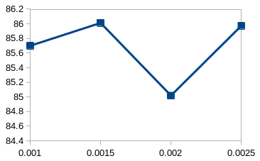
For the first experiment we transferred all but the final classification layer and trained all layers at the same learning rate as per standard transfer learning practice. We performed a search using the validation set to find the optimal single fine-tuning learning rate for each dataset. The results in Figure 1 show the accuracy for each learning rate for each dataset.
The optimal single learning rate for Caltech, the most similar dataset to ImageNet, is an order of magnitude lower than the optimal learning rate for the fine-grained classification tasks Stanford Cars and Aircraft. This shows that the optimal weights for Caltech are much closer to the pre-trained values. The surprising result was that the optimal learning rate for DTD was very similar to Caltech and also an order of magnitude lower than Stanford Cars and Aircraft. Final results on the test set for each dataset are shown in Table 2.


| Caltech | Stanford Cars | Aircraft | DTD | |
|---|---|---|---|---|
| Learning rate | 0.0025 | 0.025 | 0.025 | 0.002 |
| Accuracy | 83.690.0784 | 94.590.110 | 93.780.137 | 77.30 0.726 |
4.3 Optimal learning rate decreases as more layers are reinitialized and transferring all possible layers often reduces performance on the target task
To the best of our knowledge the combination of learning rate and number of layers reinitialized when performing transfer learning has not been examined in modern residual models. To examine the relationship between learning rate and number of layers reinitialized, we searched for the optimal learning rate for each of 1-3 blocks of layers reinitialized across each of the four datasets. One layer is the default with the final classification layer only being reinitialized. Two and three involve reinitializing an additional one or two Inception C blocks of layers respectively as well as the final layer. For consistency we refer to both the final classification layer and the Inception C blocks as layers. Figure 2 shows the performance of fine-tuning with various combinations of learning rate and layers reinitialized. The optimal learning rate when reinitializing more than one layer is always lower than when reinitializing only the final classification layer. Also the optimal number of layers to reinitialize is more than one for all datasets except Cars. Table 3 shows the final results for the optimal learning rate and accuracy for each number of layers reinitialized.
Reinitializing more layers has a more significant effect when the optimal learning rate for reinitializing just one layer is higher
Caltech and DTD have an order of magnitude lower optimal learning rates than Cars and Aircraft, but reinitializing more layers for the former results in a significant increase in accuracy whereas there is none for the latter. This result initially seems counter intuitive as Cars and Aircraft are less similar to Imagenet than Caltech and DTD. However, a lower learning rate tempers the ability of the upper layers of the model to specialise to the new domain and even very closely related source and target domains have different final classes and thus optimal feature spaces. The combination of a lower learning rate and reinitializing more layers likely allows the models to keep the closely related lower and middle layers and create new specialist upper layers.


| Caltech | Cars | Aircraft | DTD | |
|---|---|---|---|---|
| 1 layer lr | 0.0025 | 0.025 | 0.025 | 0.002 |
| Accuracy | 83.690.078 | 94.590.110 | 93.780.137 | 77.30 0.726 |
| 2 layers lr | 0.015 | 0.015 | 0.02 | 0.001 |
| Accuracy | 84.310.114 | 94.59 0.205 | 93.560.942 | 78.92 0.191 |
| 3 layers lr | 0.015 | 0.015 | 0.02 | 0.0015 |
| Accuracy | 83.570.104 | 94.460.348 | 92.961.588 | 78.900.243 |
4.4 Lower learning rates for lower layers works better when optimal learning rate is higher
Conventionally learning rates for different layers are set so that either all layers are fine-tuned with the same learning rate or some are frozen. The thinking is that as lower layers are more general and higher layers more task specific [39] the lower layers do not need to be fine-tuned. Recent work has shown that fine-tuning tends to work better in most cases [30]. However, setting different learning rates for different layers is not generally considered. We examined the effects of applying lower learning rates to lower layers that are likely to generalise better to the target task. Figure 4 shows that for the Stanford Cars and Aircraft where the optimal initial learning rate is higher, setting lower learning rates for lower layers significantly improves performance whereas for Caltech and DTD it does not.


| Caltech | Cars | Aircraft | DTD | |
|---|---|---|---|---|
| Default accuracy | 83.690.0784 | 94.590.110 | 93.780.137 | 77.300.726 |
| 1 layer lrs | 0.002 0.001 12 | 0.025 0.01 8 | 0.025 0.015 10 | 0.0025 0.0015 10 |
| Accuracy | 83.950.196 | 94.860.0460 | 94.32 0.144 | 77.7530.456 |
| 2 layers lrs | 0.002 0.001 12 | 0.025 0.01 8 | 0.025 0.015 10 | 0.0015 0.001 14 |
| Accuracy | 84.150.553 | 94.78 0.132 | 94.17 0.311 | 78.590.127 |
| 3 layers lrs | 0.002 0.001 12 | 0.025 0.01 10 | 0.01 0.025 0.01 8 | 0.0015 0.001 12 |
| Accuracy | 83.460.143 | 94.83 0.0832. | 94.50 0.192 | 78.84 0.464 |
4.5 L2SP
The L2SP regularizer decays pre-trained weights towards their pre-trained values rather than towards zero during fine-tuning. In the standard transfer learning paradigm with only the final classification reinitialized, when the L2SP regularizer is applied the final classification layer only is decayed towards 0.
The values and are tuneable hyperparameters to control the amount of regularization applied to the pre-trained and randomly initialized layers respectively.
The original experiments showing the effectiveness of the L2SP regularizer [21] were done on target datasets that are extremely similar to the source datasets used. They showed that a high level of regularization decaying towards the pre-trained weights is beneficial on these datasets. It has since been shown that the L2SP regularizer can result in minimal improvement or even worse performance when the source and target datasets are less related [18, 37].
Our results shown in Figure 4 align with the original paper [21] for the dataset Caltech showing that standard L2SP regularization does result in an improvement in performance over L2 regularization. Our results also align with [18, 37] in showing that for the datasets we have chosen to be different from Imagenet, and known to be more difficult to transfer to, L2SP regularization performs worse than L2 regularization. In general the lower the setting for alpha (the L2SP regularization hyperparameter) the better the performance.


We relaxed the binary assumption that L2SP regularization must be applied to all pre-trained layers. We used L2SP regularization for lower layers that we expected to be more similar to the source dataset and L2 regularization for upper layers to allow them to specialise to the target dataset. We searched for the optimal combinations of L2SP and L2 weight regularization along with the and hyperparameters for each dataset. We show the best settings for number of layers and amount of L2SP regularization in Table 5 and graph the optimal settings compared to the best default settings in Figure 5.
We make the following observations:
-
1.
A combination of L2SP and L2 regularization is optimal for most settings of the L2SP regularization hyperparameter () for all datasets except Caltech.
-
2.
When more layers are trained with L2 rather than L2SP regularization the optimal L2 regularization hyperparameter () is lower as the squared sum of the weights in these layers will be larger for the same model.
Further experiments were performed to search for the combination of optimal L2SP vs L2 regularization settings with optimal number of layers transferred and different learning rates for different layers. These results are also shown in Table 5.
| Caltech | Cars | Aircraft | DTD | |
|---|---|---|---|---|
| L2 | 83.694 | 94.59 | 93.78 | 77.30 |
| Default L2SP 1 new layer , | 0.01 0.01 | 0.0001 0.01 | 0.0001 0.01 | 0.0001 0.01 |
| result | 84.52 | 94.42 | 93.29 | 78.32 |
| Optimal L2SP 1 new layer , | 0.01 0.01 L2SP layers all | 0.01 0.001 L2SP layers 10 | 0.0001 0.001 L2SP layers 10 | 0.001 0.001 L2SP layers 10 |
| result | 84.52 | 94.57 | 93.86 | 78.32 |
| Optimal L2SP overall , | 0.01 0.01 L2SP layers all | 0.01 0.001 L2SP layers 10 | 0.0001 0.001 L2SP layers 10 | 0.001 0.001 1.0 L2SP layers 14 |
| result | 84.52 | 94.65 | 94.22 | 78.90 |


4.6 Final optimal settings and how to predict them
The final results and optimal settings are shown in Table 6 and Figure 6. Table 7 shows a clear distinction between target datasets that are more similar to the source dataset and for which the pre-trained weights are better able to separate the classes in feature space and those that are less similar with pre-trained weights that fit the target task poorly. The best measure for determining whether the pre-trained weights are well suited is a comparison of the performance achieved with fixed pre-trained features and that achieved through training from random initialization. As this method is computationally intensive a reasonable alternative may be the normalized Fisher Ratio, but as the differences are not as pronounced in all cases it should be further investigated on more datasets to see how reliable it is as a heuristic. The EMD measure of domain similarity is a poor predictor of the suitability of the pre-trained weights.
Targets datasets for which the pre-trained weights are well suited need:
-
•
a much lower learning rate for fine-tuning,
-
•
more than one layer to be reinitialized from random weights, and
-
•
some or all layers trained with L2SP regularization.
Target datasets where the pre-trained weights are not well suited need:
-
•
a much higher learning rate for fine-tuning with a lower learning rate for lower layers,
-
•
only the final classification layer reinitialized, and
-
•
L2 rather than L2SP regularization.
Using the above best practice, non-binary transfer learning procedures we achieved state of the art or close to, on three out of the four datasets. We used publicly available pre-trained weights and no additional methods for either pre-training or fine-tuning.
| Caltech | Cars | Aircraft | DTD | |
|---|---|---|---|---|
| Default settings | 0.0025 | 0.025 | 0.025 | 0.002 |
| Default result | 83.69 | 94.59 | 93.78 | 77.30 |
| Default L2SP | 84.52 | 94.42 | 93.29 | 78.32 |
| Optimal settings | 1 new layer lr 0.0025 L2SP 0.01 0.01 | 1 new layer high lr 0.025 low lr 0.01 low layers 8 no L2SP | 3 new layers FC lr 0.01 high lr 0.025 low lr 0.01 low layers 8 no L2SP | new layers 2 lr 0.002 L2SP 0.001 0.001 L2SP layers 14 |
| Optimal result | 84.52 | 94.86 | 94.50 | 78.90 |
| Ensemble | 85.94 | 95.35 | 95.11 | 79.79 |
| State of the art | 84.9 [20] | 96.0 (@448) [31] | 93.9 (@448) [41] | 78.9 [3] |


| Caltech | DTD | Cars | Aircraft | |
|---|---|---|---|---|
| Fisher ratio | 1.35 | 3.47 | 1.18 | 0.83 |
| EMD similarity | 0.568 | 0.540 | 0.536 | 0.557 |
| Random initialisation minus fixed features | -16.2 | -7.8 | 28.5 | 28.9 |
| Optimal learning rate | Low | Low | High | High |
| L2SP | Yes | Yes | No | No |
| More layers reinitiailized | Yes | Yes | No | No |
| Low layers at low learning rate | No | No | Yes | Yes |
5 Discussion
Traditional binary assumptions about transfer learning hyperparameters should be discarded in favour of a tailored approach to each individual dataset. These assumptions include transferring all possible layers or none, training all layers at the same learning rate or freezing some, and using L2SP regularization or L2 regularization for all layers. Our work demonstrates that optimal transfer learning non-binary hyperparameters are dataset dependent and strongly influenced by how well the pre-trained weights fit the target task. For a particular dataset, optimal non-binary transfer learning hyperparameters can be determined based on the difference between model performance when fixed features are used and when the full model is trained from random initialization as shown in Table 7. We recommend using the settings shown on the left in this table for target datasets where the difference is negative and settings shown on the right for positive differences. Target datasets for which the pre-trained weights are well suited and target datasets for which they are not result in large differences in this value. These differences should still be pronounced even if suboptimal learning hyperparameters are used for this initial test due to limited resources for hyperparameter search. This heuristic for determining optimal hyperparameters should be useful in most transfer learning for image classification cases. The normalized Fisher Ratio may be useful in some cases, however, care should be taken because the differences are not as pronounced. The EMD domain similarity measure should not be used to determine transfer learning hyperparameters.
6 Broader Impact
This research is focused on improving transfer learning for small target image classification datasets. The positive impacts are easy to observe in improved performance of models utilising transfer learning in a wide range of real world applications. For example, faster and more accurate medical diagnostics where there is limited data available.
However, improvements to image classification models can have positive or negative impacts. More accurate models could reduce errors but result in overconfidence and more reliance on results in areas where the full limitations are not well understood and taken into account. Improved image classification models could also be used in areas with potential negative impacts, for example:
-
•
use of intrusive facial recognition systems
-
•
discrimination based on subtle items such as religious symbols
7 Limitations and future work
The main aim of this work is to highlight the need for a non-binary approach to achieving optimal performance in transfer learning applied to image classification on small target datasets. The relationship between the source and the target dataset and how well the pre-trained weights fit the target task has been shown to be important to transfer learning performance numerous times [28, 22, 6, 8, 33, 21, 20, 37, 27, 42, 18]. However, the guidance as to how to set transfer learning hyperparameters based on the heuristics presented in this paper is based only on the experiments on the four datasets outlined in this paper. Care should be taken if applying this guidance to new datasets, particularly outside of image classification.
References
- [1] Pulkit Agrawal, Ross Girshick, and Jitendra Malik. Analyzing the performance of multilayer neural networks for object recognition. In European conference on computer vision, pages 329–344. Springer, 2014.
- [2] Hossein Azizpour, Ali Sharif Razavian, Josephine Sullivan, Atsuto Maki, and Stefan Carlsson. Factors of transferability for a generic convnet representation. IEEE transactions on pattern analysis and machine intelligence, 38(9):1790–1802, 2015.
- [3] Ting Chen, Simon Kornblith, Mohammad Norouzi, and Geoffrey Hinton. A simple framework for contrastive learning of visual representations. In International conference on machine learning, pages 1597–1607. PMLR, 2020.
- [4] Brian Chu, Vashisht Madhavan, Oscar Beijbom, Judy Hoffman, and Trevor Darrell. Best practices for fine-tuning visual classifiers to new domains. In European conference on computer vision, pages 435–442. Springer, 2016.
- [5] Mircea Cimpoi, Subhransu Maji, Iasonas Kokkinos, Sammy Mohamed, and Andrea Vedaldi. Describing textures in the wild. In Proceedings of the IEEE Conference on Computer Vision and Pattern Recognition, pages 3606–3613, 2014.
- [6] Yin Cui, Yang Song, Chen Sun, Andrew Howard, and Serge Belongie. Large scale fine-grained categorization and domain-specific transfer learning. In Proceedings of the IEEE conference on computer vision and pattern recognition, pages 4109–4118, 2018.
- [7] K Fukenaga. Introduction to statistical pattern recognition. 2ed, Academic Press, San Diego, 1990.
- [8] Weifeng Ge and Yizhou Yu. Borrowing treasures from the wealthy: Deep transfer learning through selective joint fine-tuning. In Proceedings of the IEEE conference on computer vision and pattern recognition, pages 1086–1095, 2017.
- [9] Ross Girshick, Jeff Donahue, Trevor Darrell, and Jitendra Malik. Rich feature hierarchies for accurate object detection and semantic segmentation. In Proceedings of the IEEE conference on computer vision and pattern recognition, pages 580–587, 2014.
- [10] Gregory Griffin, Alex Holub, and Pietro Perona. Caltech256 object category dataset. California Institute of Technology, 2007.
- [11] Yunhui Guo, Honghui Shi, Abhishek Kumar, Kristen Grauman, Tajana Rosing, and Rogerio Feris. Spottune: transfer learning through adaptive fine-tuning. In Proceedings of the IEEE Conference on Computer Vision and Pattern Recognition, pages 4805–4814, 2019.
- [12] Kaiming He, Ross Girshick, and Piotr Dollár. Rethinking imagenet pre-training. arXiv preprint arXiv:1811.08883, 2018.
- [13] Kaiming He, Xiangyu Zhang, Shaoqing Ren, and Jian Sun. Deep residual learning for image recognition. In Proceedings of the IEEE conference on computer vision and pattern recognition, pages 770–778, 2016.
- [14] Alexander Kolesnikov, Lucas Beyer, Xiaohua Zhai, Joan Puigcerver, Jessica Yung, Sylvain Gelly, and Neil Houlsby. Big transfer (bit): General visual representation learning. arXiv preprint arXiv:1912.11370, 2019.
- [15] Simon Kornblith, Jonathon Shlens, and Quoc V Le. Do better imagenet models transfer better? In Proceedings of the IEEE Conference on Computer Vision and Pattern Recognition, pages 2661–2671, 2019.
- [16] Jonathan Krause, Michael Stark, Jia Deng, and Li Fei-Fei. 3d object representations for fine-grained categorization. In 4th International IEEE Workshop on 3D Representation and Recognition (3dRR-13), Sydney, Australia, 2013.
- [17] Alex Krizhevsky, Ilya Sutskever, and Geoffrey E Hinton. Imagenet classification with deep convolutional neural networks. In Advances in neural information processing systems, pages 1097–1105, 2012.
- [18] Hao Li, Pratik Chaudhari, Hao Yang, Michael Lam, Avinash Ravichandran, Rahul Bhotika, and Stefano Soatto. Rethinking the hyperparameters for fine-tuning. arXiv preprint arXiv:2002.11770, 2020.
- [19] Shan Li and Weihong Deng. Deep facial expression recognition: A survey. IEEE Transactions on Affective Computing, 2020.
- [20] Xingjian Li, Haoyi Xiong, Hanchao Wang, Yuxuan Rao, Liping Liu, and Jun Huan. Delta: Deep learning transfer using feature map with attention for convolutional networks. arXiv preprint arXiv:1901.09229, 2019.
- [21] Xuhong Li, Yves Grandvalet, and Franck Davoine. Explicit inductive bias for transfer learning with convolutional networks. arXiv preprint arXiv:1802.01483, 2018.
- [22] Dhruv Mahajan, Ross Girshick, Vignesh Ramanathan, Kaiming He, Manohar Paluri, Yixuan Li, Ashwin Bharambe, and Laurens van der Maaten. Exploring the limits of weakly supervised pretraining. In Proceedings of the European Conference on Computer Vision (ECCV), pages 181–196, 2018.
- [23] S. Maji, J. Kannala, E. Rahtu, M. Blaschko, and A. Vedaldi. Fine-grained visual classification of aircraft. Technical report, Toyota Technological Institute at Chicago, 2013.
- [24] Iacopo Masi, Yue Wu, Tal Hassner, and Prem Natarajan. Deep face recognition: A survey. In 2018 31st SIBGRAPI conference on graphics, patterns and images (SIBGRAPI), pages 471–478. IEEE, 2018.
- [25] Maciej A Mazurowski, Mateusz Buda, Ashirbani Saha, and Mustafa R Bashir. Deep learning in radiology: An overview of the concepts and a survey of the state of the art with focus on mri. Journal of magnetic resonance imaging, 49(4):939–954, 2019.
- [26] Romain Mormont, Pierre Geurts, and Raphaël Marée. Comparison of deep transfer learning strategies for digital pathology. In Proceedings of the IEEE Conference on Computer Vision and Pattern Recognition Workshops, pages 2262–2271, 2018.
- [27] Hong-Wei Ng, Viet Dung Nguyen, Vassilios Vonikakis, and Stefan Winkler. Deep learning for emotion recognition on small datasets using transfer learning. In Proceedings of the 2015 ACM on international conference on multimodal interaction, pages 443–449, 2015.
- [28] Jiquan Ngiam, Daiyi Peng, Vijay Vasudevan, Simon Kornblith, Quoc V Le, and Ruoming Pang. Domain adaptive transfer learning with specialist models. arXiv preprint arXiv:1811.07056, 2018.
- [29] Shmuel Peleg, Michael Werman, and Hillel Rom. A unified approach to the change of resolution: Space and gray-level. IEEE Transactions on Pattern Analysis and Machine Intelligence, 11(7):739–742, 1989.
- [30] Jo Plested and Tom Gedeon. An analysis of the interaction between transfer learning protocols in deep neural networks. In International Conference on Neural Information Processing, pages 312–323. Springer, 2019.
- [31] Tal Ridnik, Hussam Lawen, Asaf Noy, and Itamar Friedman. Tresnet: High performance gpu-dedicated architecture. arXiv preprint arXiv:2003.13630, 2020.
- [32] Yossi Rubner, Carlo Tomasi, and Leonidas J Guibas. The earth mover’s distance as a metric for image retrieval. International journal of computer vision, 40(2):99–121, 2000.
- [33] Matthia Sabatelli, Mike Kestemont, Walter Daelemans, and Pierre Geurts. Deep transfer learning for art classification problems. In Proceedings of the European Conference on Computer Vision (ECCV), pages 0–0, 2018.
- [34] Zhiqiang Shen, Zhuang Liu, Jianguo Li, Yu-Gang Jiang, Yurong Chen, and Xiangyang Xue. Dsod: Learning deeply supervised object detectors from scratch. In Proceedings of the IEEE international conference on computer vision, pages 1919–1927, 2017.
- [35] Zhiqiang Shen, Honghui Shi, Rogerio Feris, Liangliang Cao, Shuicheng Yan, Ding Liu, Xinchao Wang, Xiangyang Xue, and Thomas S Huang. Learning object detectors from scratch with gated recurrent feature pyramids. arXiv preprint arXiv:1712.00886, 1, 2017.
- [36] Christian Szegedy, Sergey Ioffe, Vincent Vanhoucke, and Alexander A Alemi. Inception-v4, inception-resnet and the impact of residual connections on learning. In Thirty-First AAAI Conference on Artificial Intelligence, 2017.
- [37] Ruosi Wan, Haoyi Xiong, Xingjian Li, Zhanxing Zhu, and Jun Huan. Towards making deep transfer learning never hurt. In 2019 IEEE International Conference on Data Mining (ICDM), pages 578–587. IEEE, 2019.
- [38] Ross Wightman. Pytorch image models. https://github.com/rwightman/pytorch-image-models, 2019.
- [39] Jason Yosinski, Jeff Clune, Yoshua Bengio, and Hod Lipson. How transferable are features in deep neural networks? In Advances in neural information processing systems, pages 3320–3328, 2014.
- [40] Rui Zhu, Shifeng Zhang, Xiaobo Wang, Longyin Wen, Hailin Shi, Liefeng Bo, and Tao Mei. Scratchdet: Training single-shot object detectors from scratch. In Proceedings of the IEEE conference on computer vision and pattern recognition, pages 2268–2277, 2019.
- [41] Peiqin Zhuang, Yali Wang, and Yu Qiao. Learning attentive pairwise interaction for fine-grained classification. In Proceedings of the AAAI Conference on Artificial Intelligence, number 07 in 34, pages 13130–13137, 2020.
- [42] Barret Zoph, Golnaz Ghiasi, Tsung-Yi Lin, Yin Cui, Hanxiao Liu, Ekin D Cubuk, and Quoc V Le. Rethinking pre-training and self-training. arXiv preprint arXiv:2006.06882, 2020.