Response Theory Identifies Reaction Coordinates and Explains Critical Phenomena in Noisy Interacting Systems
Abstract
We consider a class of nonequilibrium systems of interacting agents with pairwise interactions and quenched disorder in the dynamics featuring, in the thermodynamic limit, phase transitions. We provide conditions on the microscopic structure of interactions among the agents that lead to a dimension reduction of the system in terms of a finite number of reaction coordinates. Such reaction coordinates prove to be proper nonequilibrium thermodynamic variables as they carry information on correlation, memory and resilience properties of the system. Phase transitions can be identified and quantitatively characterised as singularities of the complex valued susceptibility functions associated to the reaction coordinates. We provide analytical and numerical evidence of how the singularities affect the physical properties of finite size systems.
Keywords: Multiagent models, Critical phenomena, Resilience, Collective variables, Statistical mechanics, Linear Response, Nonequilibrium systems
1 Introduction
Interacting agent models are at the basis of the microscopic description of the rich variety of collective emergent phenomena that high dimensional complex systems often exhibit. Common applications of such models range from synchronisation of nonlinear oscillators [1, 2, 3, 4, 5, 6, 7, 8], see also the recent special issue [9], phase transitions in complex energy landscapes [10, 11] to opinion dynamics and consensus formation [12, 13], socio-economic siences [14, 15], life sciences [16], the dynamics of the brain [17], formation of swarms [18, 19], dynamical networks [20], self-gravitating systems [21, 22] and algorithms for optimisation and training of neural networks [23, 24, 25]. In the thermodynamic limit, such systems can exhibit phase transitions resulting from the interplay between the interaction among the agents, their internal dynamics and the noise. Such critical phenomena are associated with the so called critical slowing down phenomenon, that is by long lasting, persistent fluctuations exhibiting statistics far away from Gaussianity, see [26] for a detailed description of the critical fluctuations for an equilibrium continuous phase transition.
1.1 From a microscopic to a macroscopic description of the system
From an operational point of view, the investigation of these critical phenomena heavily relies on the identification of a suitable set of observables, commonly referred to as order parameters (OPs), collective variables (CVs) or reaction coordinates (RCs), acting as thermodynamic variables by providing a low dimensional description of the macroscopic feature of the system. Whereas it is true that all the three notions of OP, CV and RC are related to a dimension reduction procedure provided by a projection from a high dimensional system to a reduced state space, they refer to different features of the system. Along the lines of [27], we define a CV as any function of the full phase space. An OP is then a suitable combination of CVs that is able to distinguish between macroscopic, possibly metastable, states of the sytem. As some relevant parameters of the system are varied, one wishes to identify critical points by observing asymptotic properties of the OPs, that is by constructing phase diagrams. On the other hand, the term RC refers to a suitable OP that is able to capture time dependent properties of the system, e.g. relaxation phenomena or transitions between metastable states.
A major challenge in the identification of critical phenomena is that, while order parameters or reaction coordinates can in many cases be deduced for equilibrium systems using, e.g., symmetry arguments, the identification of reaction coordinates in nonequilibrium settings is far less trivial [28, 29, 27] and is tailored to the specific problem at hand.
Here we provide a constructive, as opposed to ad hoc, criterion to identify a set of reaction coordinates for a large class of interacting agent systems based on the microscopic interaction structure among the agents. Inspired by the success of response theory in explaining critical phenomena in a class of interacting systems [30, 31, 32, 33], we show that, according to this perspective, the not only represent OPs for the system but correspond to suitable RCs as they act as proper nonequilibrium thermodynamic variables. On the one hand, their stationary asymptotic properties identify the different macroscopic states of the system. On the other hand, they also carry information on correlation properties and resilience of the system to perturbations. Most importantly, we show that such observables represent the optimal observables to fully characterise the development of a critical phenomenon as the critical, strongly peaked, resonances in their linear response to external perturbations allow for a quantitative description of the critical behaviour.
1.2 Linear Response
Linear Response Theory provides a powerful framework to predict how statistical properties of a system change as a result of weak, yet arbitrary exogenous perturbations. Originally developed for statistical mechanical systems near equilibrium, the theory has much larger validity [34] with applications ranging from driven, strongly dissipative systems such as the climate [35, 36] to neural networks [37, 38, 39] and financial markets [40]. In brief, a linear response perspective corresponds to the following conceptual and mathematical framework. Given a system with a unique, physical, ergodic (not necessarily smooth) measure , linear response theory aims at evaluating changes in the expectation value
| (1) |
where is a generic observable of the system, is a typical trajectory and the last equality hold because of ergodicity. Linear response theory is valid for a vast class of systems ranging from deterministic dynamical systems [34, 41], Markov chain models [42] to continuous stochastic systems [43, 44] where it can be justified on rigorous mathematical grounds [45]. We here consider a finite dimensional system described by a set of Ito stochastic differential equations with deterministic drift and noise law given by the matrix valued function
| (2) |
where is a dimensional Wiener process. If we assume that the stochastic process is hypoelliptic [44], the invariant measure associated to the above stochastic process is absolutely continuous with respect to the Lebesgue measure with smooth probability density , that is , even when the deterministic drift induces a chaotic dynamics. We perturb the system by letting where the bounded function represents the time modulation of the external perturbation and its phase space state dependence. In this setting, the statistical properties of the system change as
| (3) |
where is the Green’s function associated to the observable . The Green’s function encodes all the positive and negative feedbacks of the system and allows to evaluate the response of the system to general time dependent forcings. Response formulas provide a useful decomposition of any Green’s function as111In expression (4) the contribution of the continuous part of the spectrum is neglected, which is equivalent to assuming that the Markov semigroup describing the dynamics is quasi compact [46].
| (4) |
where the complex valued exponential rates and are the eigenvalues of the generator of the Markov semigroup associated to the unperturbed dynamics (2) and are referred to as stochastic Ruelle Pollicott resonances and are suitable coefficients [47, 48, 49]. Moreover, if the eigenvalue is not simple, that is its multiplicity is , modulating polynomial terms arise in the expression for the Green’s function.
We remark that the exponential rates represent an intrinsic property of the unperturbed dynamics and correspond to natural relaxation and oscillatory timescales of the system. Green’s functions are thus the relevant quantities to be investigated in order to detect the onset of critical instabilities of general systems. In the context of interacting systems, it has been shown that long lasting and persistent modes with exponential rates of small real part are associated to poorly damped instabilities due to phase transitions in the thermodynamic limit [31].
It is important to stress that the choice of the observable under investigation remains a critical issue in detecting criticalities as the coefficients are not an intrinsic property of the system but depend both on the observable and the state dependence of the perturbation [47]. In particular, if the observable has vanishingly small projection on the most unstable mode, its associated Green’s function would not represent a good proxy for the detection of the critical behaviour of the system.
1.3 This paper
The main contributions of this paper can be summarised as follows:
-
•
We provide a constructive way to define a finite set of RCs for the thermodynamic limit of an ensemble of interacting agents. The RCs correspond to an effective dimension reduction of the system in terms of a few relevant observables. We provide mathematical conditions on the interaction structure among the agents for which the construction of RCs is exact. In the context of synchronisation phenomena for ensembles of phase oscillators with purely harmonic coupling, dimension reduction is usually obtained by invoking the Ott-Antonsen ansatz and generalisations thereof [50, 51, 52, 53]. Our results are instead valid for any coupling structure and even in settings where phase reduction techniques of nonlinear oscillators [54, 55] cannot be applied. In this context, this paper represents a generalisation of [6] to settings with (a) possibly multiplicative, white noise sources and (b) an interaction structure that is not a priori assumed to depend on (functions of) the empirical mean of the ensemble.
-
•
We derive response formulas for the thermodynamic limit of the ensemble of agents. We show that the response of general mean field observables of the system is mediated by these RCs. In particular, we show that the coupling among the agents manifest itself in the thermodynamic limit as a memory contribution, conveyed by the RCs, to the sensitivity properties of the system. We prove that the macroscopic Green’s function describing the response of the system at a macroscopic level encodes feedbacks stemming from both microscopic properties of each agent and the interaction structure among them.
-
•
We show that the investigation of criticalities arising from phase transitions are associated, in the thermodynamic limit, to the divergent behaviour of Green’s functions relative to the RCs. Phase transitions can be quantitatively identified as the singular part of the complex valued susceptibility, the Fourier Transform of the Green’s Function. These singularities can be characterised by a pole-residue pair with and . The pole corresponds to frequencies of the driving force that would critically destabilise the system, whereas the residue determines the strength and detailed nature of the singularity.
-
•
We provide analytical and numerical evidence that the analysis of response properties of the RCs in a finite size ensemble of agents is able to capture the signature of a phase transition as a resonance around the singular thermodynamic behaviour. We show that both the pole and the residue can be inferred in a finite system. In particular, we illustrate the physical role that the residue plays on response properties of the system.
The paper is structured as follows. In section 2 we introduce the class of interacting systems under investigation and we describe when a dimension reduction in terms of RCs is possible. Section 3 is dedicated to the description of linear response properties of the system in terms of the RCs. In section 4 we investigate the critical response properties of a finite ensemble of Kuramoto oscillators. In the conclusions we mention future research directions of this linear response framework to investigate resilience features of general interacting systems.
2 The interacting agent models
We consider an ensemble of interacting -dimensional systems whose dynamics is described by the following stochastic differential equations
| (5) |
The smooth vector field , possibly depending on a set of parameters , defines the local dynamics of each agent corresponding to, in general, nonequilibrium, dissipative conditions.The (pair-wise) interactions among the systems are introduced via the function with representing the coupling strength. The function is assumed to be antisymmetric in its arguments, , to model Newton’s third law of motion for the internal forces acting between the systems. The volatility matrix determines the state dependent noise term, with being its amplitude and representing a Brownian motion. In the following we will adopt the Itô’s convention. Furthermore, we introduce a source of quenched disorder by letting the function depend on a vector of parameters drawn from a fixed known distribution , that is . The microscopic architecture of the system given by can be interpreted either as an intrinsic property of the system, such as the natural frequencies of an ensemble of oscillators, or as a model error feature arising from partial knowledge of the microscopic properties of the agents.
In the thermodynamic limit , the mean field nature of the coupling allows to obtain a macroscopic hydrodynamic description of the ensemble of agents [56, 57, 58]. More specifically, we define the empirical density of the particle system as , where represents the Dirac delta distribution. Under general conditions, it is possible to show that the system exhibits propagation of molecular chaos [16, 59], i.e. , fixed and given a chaotic initial condition , the empirical density converges weakly to where the the one-particle distribution satisfies the nonlinear Fokker Planck Equation (NFPE)
| (6) |
where and . In equation (6) the drift term depends on the probability distribution itself through originating from the coupling among the agents and represents the state dependent diffusive part. We remark that the microscopic architecture of the system manifests itself in equation (6) as an expectation value over the distribution . In particular, the homogeneous case where no quenched disorder is present is obtained by setting where is a constant parameter. We observe that equation (9) represent a nonlinear and nonlocal (integro-differential) equation and can thus support multiple coexisting stationary measures, corresponding to different macroscopic state of the system. Furthermore, exchange of stability of such measures, as the parameters of the system are varied, correspond to phase transition for the system [60, 20].
We remark that the phenomenon of propagation of molecular chaos stated above is equivalent to a mean field approximation of the Fokker Planck associated to (5), where the N-particle probability distribution is assumed to be factorised as a product of one-particle distributions . This corresponds to the simplest closure scheme, characterised by considering all agents as statistically independent, of the BBGKY hierarchy [61], an infinite set of equations describing the correlations among the N subsystems. It is known that, at a phase transition point, correlations can no longer be neglected at a macroscopic level [26]. Thus, near a phase transition point the NFPE is not expected to capture the behaviour of fluctuations, correlation and relaxation properties of macroscopic observables. We mention that the Linear Response perspective described later in section 3 and 4 can be interpreted as an approach to characterising critical fluctuations.
2.1 Identification of Reaction Coordinates
Equation (6) represents a coarse grained, mesoscopic, description of the system valid for a big, strictly infinite, ensemble of agents. However, even at this coarse grained level, this equation represents an infinite dimensional problem as the drift coefficient depends on the full one-particle probability distribution through the convolution product . It is then fundamental to find conditions on the dynamics of the system for which suitable OPs or RCs can be found. It turns out that the characterisation of RCs for these systems is strictly related to the properties of the interaction kernel . We consider a separable interaction kernel, that is, admitting a decomposition
| (7) |
where , . We remark that it is always possible to assume that the functions in the above decomposition are linearly independent [62]. In this case, the effect of the nonlinearity in equation (6) can be written in terms of a finite number of suitable observables rather than on the full probability distribution since, using (7), the interaction term results in
| (8) |
where represents the double expectation value with respect to and . Equation (6) can now be written as
| (9) |
where is a finite vector ( not necessarily equals to and , see later discussion) of observables and are linearly independent functions. We have also defined the nonlinear operator depending on the probability distribution through the vector . Following the terminology of [60], this scenario corresponds to a finite nonlinearity dimension equals to for equation (6) and it corresponds to a natural dimension reduction of the ensemble of agents in terms of the variables .
Separable kernels arising from interaction potentials are routinely used in applications, with radial potentials of the form being a common choice. A paradigmatic example is represented by quadratic interactions , yielding a separable kernel . This corresponds to linear forces among the particles trying to synchronise them towards their centre of mass and has numerous applications, see our previous work [30, 31] on this. In this case, , the expansion (7) of the interaction kernel holds with and resulting in a non linear dimension for equation (9) given by the observables . Similarly, higher order polynomials with give rise to separable kernels and a finite nonlinearity dimension. As a further example, we mention separable kernels provided by trigonometric interactions of any order with applications to synchronisation phenomena, see [63, 8] and the section below on the Kuramoto model. We refer the reader to the conclusions section for a discussion regarding non separable kernels.
We remark that equation (9) can be interpreted as a thermodynamic formulation of the system with the s being a generalisation of thermodynamic variables to nonequilibrium settings [64]. Firstly, stationary distributions of (9) can be parametrised in terms of the stationary values of the thermodynamic variables according to the self consistency equation given by the stationary condition where is the operator defined in (9) evaluated at stationarity.
This is better understood in the case of homogeneous equilibrium systems, characterised by a gradient dynamics , an interaction potential , thermal noise and no quenched disorder. In such systems, stationary solutions of (6) satisfy the self consistency equation [20]
| (10) |
where is a normalisation constant. Assuming a separable kernel, equilibrium stationary solutions are parametrised by a finite number of observables since they can be written as where is a suitable function deriving by the convolution product , similarly to equation (8).
Moreover, the s represent proper RCs of the system as they govern time dependent properties of the ensemble of agents, such as its response, correlation and memory features, as we elucidate in the next section.
3 Response Formulas
We remark that a stationary state of equation (9) is characterised by the constant set of observables , where the subscript denotes that the expectation value is taken with respect to (and ). We perturb such state with a time and state dependent perturbation by letting and we write . We observe that, since , where the last subscript denotes the expectation value with respect to , the perturbation to the nonlinear part of the drift term can be written as
| (11) |
where the matrix provides the information on how the drift term changes, in a linear approximation, with respect to the observables and is defined as
| (12) |
From (9) we obtain an equation for the perturbation to the stationary measure
| (13) |
where is the perturbation operator. We now evaluate the perturbation to the observable by taking the expected value with respect to and to obtain
| (14) |
where denotes the convolution product and we have defined the microscopic Green’s functions
| (15a) | ||||
| (15b) | ||||
We observe that depends on the perturbation whereas does not, representing thus an intrinsic property of the system describing its internal feedbacks, see [30]. The coupling among the agents manifests itself as a memory term in (14) conveyed by the variables through the microscopic Green’s Function . Taking the Fourier transform of (14) we obtain
| (16) |
where we have defined the matrix
| (17) |
and () are the Fourier transform of the microscopic Green functions () respectively. Equations (16) and (17) completely characterise the response of statistical properties of the system to perturbations in terms of the observables . When is an analytic function in the upper complex plane and is invertible the response of the system is smooth and given by
| (18) |
where is the complex valued macroscopic susceptibility associated to the RCs. In this case, , the inverse Fourier transform of , defines a causal macroscopic Green’s function describing the response properties of the system as
| (19) |
From an operational point of view, the macroscopic Green’s function is the quantity that is experimentally accessible at a macroscopic level. This function encodes all positive and negative feedbacks of the system, including feedbacks stemming from microscopic single agent features and from the interaction among them. We remark that the macroscopic Green’s function , being the inverse Fourier transform of the macroscopic susceptibility defined in (18), has a non trivial expression in terms of the microscopic Green’s function and .
Criticalities in the response of the system arise when the negative feedbacks are no longer successful in damping the external perturbations and are signalled by the fact that some modes of the macroscopic Green’s function do not decay in time. More specifically, the response of the system breaks down as a result of a pole in when either develops a singularity, corresponding to a destabilisation of each agent in the system [30], or when becomes noninvertible. Equation (17) shows that the latter case arises due to endogenous instabilities associated with positive feedbacks resulting from the coupling among the agents. This identifies the occurrence of a phase transition in the system as it is intimately related to taking the thermodynamic limit [30]. We remark that, generally, a linear stability analysis of nonlinear Fokker Planck equations such as (9), e.g. for the Kuramoto model described below, involves the investigation of spectral properties of (infinite dimensional) linear integral operators [60, 65]. However, the identification of RCs allows to simplify the stability problem into the analysis of the finite dimensional matrix encoding their intrinsic response properties.
4 Critical phenomena for the Kuramoto model
We elucidate the above results by investigating critical phenomena in the Kuramoto model [65, 66], the paradigmatic example of synchronisation phenomena of phase oscillators. We remark that, even if the Kuramoto model has been thoroughly investigated, a stability theory of the stationary solutions of the Kuramoto model is still lacking, see [67] for partial results in this direction in deterministic settings. The goal of this section is to shed light on the physical mechanisms underlying the onset of synchronisation encoded in the properties of the Green’s function of the system. In particular, we are interested in showing how the critical response of a finite dimensional system relates to the properties of the complex valued susceptibility .
The Kuramoto model is defined by the following SDEs
| (20) |
where the quenched disorder in this case corresponds to the presence of a non-trivial distribution of intrinsic frequencies across the oscillators, so that . The interaction kernel is separable and leads, in the thermodynamic limit, to the following NFPE of nonlinearity dimension
| (21) |
where and represents the set of reaction coordinates for the system. The uniform distribution is always a solution of equation (21) corresponding to a incoherent state characterised by a set of reaction coordinates . We here focus on the task of assessing the response properties of the incoherent state . From (12), we evaluate yielding222We refer the reader to the Appendix for the details regarding the calculations regarding this section. the microscopic Green’s Function :
| (22) |
where and is the correlation function in the stationary state between observable and . If we consider an even distribution of intrinsic frequencies the matrix (17) is diagonal and
| (23) |
where is the Fourier Transform of the (diagonal part of the) correlation function and the explicit expressions for and are in the Appendix. Singularities in the response of the reaction coordinate , due to a phase transition, are characterised by a value such that the matrix is not invertible, or, equivalently, such that . Separating real and imaginary part of results respectively in
| (24a) | ||||
| (24b) | ||||
Equation (24b) determines the critical value whereas (24a) identifies the corresponding transition point in the parameter space . An immediate solution of (24b) is , which takes place, according to (24a), at the critical coupling strength in agreement with [68].
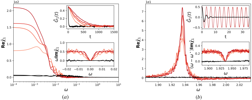
This setting corresponds to a static phase transition, characterised by a vanishing pole of the susceptibility and a lack of oscillations in the system, see panel (a) of Figure 1 where we have investigated this scenario for . The introduction of a distribution of natural frequencies brings the system to a nonequilibrium regime and it is interesting to investigate whether a dynamical phase transition, characterised by a pair of poles , can arise in the system. This involves the study of the dynamical properties encoded in . Further insight can be gained by observing that, if (24b) is satisfied for , the following equation holds, see details in the Appendix,
| (25) |
which is a known result for the Kuramoto model [66]. In particular, no dynamical phase transition can take place if is unimodal as no satisfying (25) exists. We here consider, as in [69], a bimodal distribution . In this setting, equation (24b) admits, further to the static transition scenario, a new solution when . According to (24a), this dynamical phase transition scenario takes place at the transition point . Panel (b) of Figure 1 confirms that, at the phase transition, response properties break down as the susceptibility develops a singular resonant behaviour for as , resulting in greatly amplified and long lasting oscillations of the macroscopic Green’s function .
4.1 Response properties of the finite system
Following [43], we evaluate response properties of the finite system by performing simulations of equations (20) where the initial conditions are sampled according to and where at time we apply a macroscopic perturbation . The macroscopic Green’s function is obtained as the average over the ensemble members of which we estimate as . We remark that, since the unperturbed measure is uniform, a constant perturbation would result in a vanishing response as , see (15a). We have here chosen a non trivial state dependent perturbation . We note that such term has been used to model excitability features in Kuramoto-like models for brain dynamics [70]. The numerical experiments indicate that the finite system susceptibility can be written, at the phase transition, as
| (26) |
where is an analytic function in the upper complex plane and the residue characterises the strength of the divergence. The residue is related to the properties of and can be found as , see Appendix for more details.
We remark that the finiteness of the system results in a mollifying effect of the singularity into a resonant behaviour, where the poles are slightly shifted as , with as . In the homogeneous case the residue turns out to be completely imaginary and equal to , whereas for the bimodal case it results in . In the former case, one expects that, as , the function will be constant and equal to in the proximity of the pole and to quickly drop to zero for . A visual inspection of the bottom inset of panel (a) of Figure 1 provides a clear evidence of such theoretical prediction.
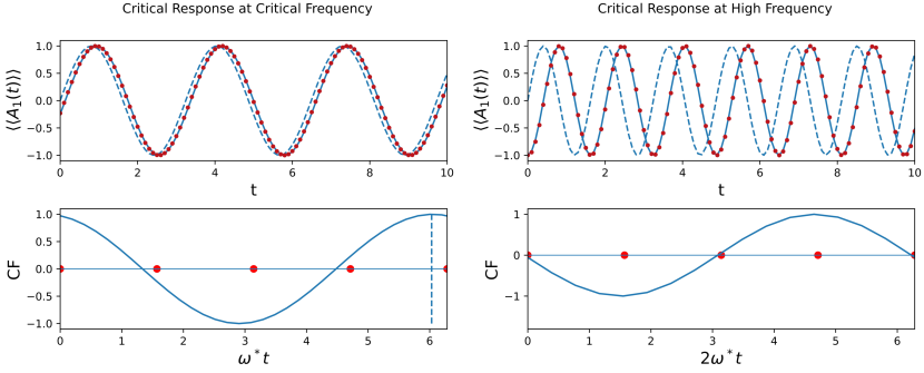
A fundamentally different situation occurs in the latter case as the residue has a non-vanishing real part leading to a distortion of the resonance at as and, thus, affecting the way the amplitude of the oscillations of the response track the forcing signal. This is more easily understood when considering a sinusoidal driving forcing . The response (in the time domain) can be obtained by performing an inverse Fourier transform of (18) and results in
| (27) |
The amplitude of the response is given by the amplitude of the macroscopic susceptibility. We expect that driving frequencies around the pole would destabilise the system resulting in greatly amplified oscillations, whereas the system would be much more resilient for higher driving frequencies. Moreover, if the imaginary part of the susceptibility were to vanish, the response would feature either no phase shift as or phase reversal as . At the critical frequency we have, from (26), that the response is given by with . The non vanishing real part of the residue yields a spontaneous phase shift of the response to perturbations as confirmed by Figure 2 (left panels). We remark that this provides a quantitative estimate, at the phase transition, of the phase shift phenomenon observed (in deterministic settings) in [71]. On the other hand, if the system is driven at higher frequency, e.g. , we expect the real part of the susceptibility to decay faster than the imaginary part [72] and the response to be in quadrature with the forcing, i.e. , as confirmed by Figure 2 (right panels).
4.2 Conclusions
In this paper we have considered the relevant issue of the identification of a set of reaction coordinates for the thermodynamic limit of ensembles of interacting agents in the general case of pairwise interaction and quenched disorder in the dynamics. Given a general class of interaction structure among the agents, we have provided a framework to define the and construct a nonequilibrium thermodynamical formulation of the macroscopic description of the system. These reaction coordinates provide a parametrization of the stationary measure and fully characterise the linear response of the system to perturbations. Such a model reduction strategy is particularly useful as it allows to study not only smooth regimes of the response but also critical behaviours, characterised as an emergence of singular poles of the complex valued susceptibility of the system. The analysis in terms of the reaction coordinates of the paradigmatic Kuramoto model allows us to show (a) that our framework encompasses known results on the stability properties of the incoherent state and (b) that the time dependent properties of the onset of synchronisation can be quantitatively investigated through the susceptibility function describing the response of the system to general driving forces.
Our results are exact in the case of separable interactions. However, non separable kernels are also found in applications. If is a smooth function, an expansion as in (8) still holds by using a Schauder decomposition [73] but it contains in general an infinite number of terms, resulting in an infinite number of observables with a clear loss of dimension reduction of the system. However, there exist numerous rigorous techniques to approximate in a controlled manner a general kernel in terms of suitable separable kernels, see [62, Ch. 11][74]. Such approximating methods would be the basis for the development of phenomenological theories of interacting systems with suitable separable interactions for which the identification of a finite number of observables can be performed exactly.
On the one hand, the investigation of mean field models is very relevant as it provides a way of gaining a mathematical and analytical understanding of the smooth and critical features of ensembles of interacting agents. On the other hand, the lack of an underlying geometrical structure might pose a too restrictive limitation to the applications of these models. Future research in this direction will involve the generalisation of this framework to systems with a microscopic network structure [75] and in particular to all systems amenable to a description in terms of graphon [76, 77] and graphop theory [78, 79]. We envision that this framework can be extended to include the physically relevant cases where the dynamics is not assumed to be overdamped, in the direction of understanding nonequilibrium ensembles in statistical mechanics [80] and to non-Markovian interacting particles [81], where appropriate Markovian closures have to be considered [44, 82].
Appendix A Dynamical Properties of the Kuramoto model
We provide here the detailed calculations leading to the results reported in the main text regarding the Kuramoto model. This model describes an ensemble of one dimensional () phase oscillators on the torus whose dynamics is determined by the following Stochastic Differential Equations
| (28) |
where , with , represents the intrinsic frequencies of each oscillator and the symbols are defined as in the main text. The interaction kernel is separable and leads, in the thermodynamic limit [16, 59], to the following nonlinear nonlocal Fokker Planck equation of nonlinearity dimension
| (29) |
where where represents the set of reaction coordinates for the Kuramoto model. It is easy to verify that the uniform solution is always a stationary solution of equation (29) corresponding to a disordered state characterised by a set of observables . Moreover, this stationary solution satisfies where
| (30) |
Below we investigate the response properties of the disordered state and detect phase transitions of the system by looking at the singularities of the susceptibility of the system originating from non invertibility properties of the matrix , see equation in the main text. We evaluate the matrix (here a vector since )
| (31) |
Considering that , the microscopic Green’s function can be written as where
| (32) |
Now, it is easy to verify that
| (33) |
where and
| (34) |
The microscopic Green Function can then be written as
| (35) |
where is the correlation function between observable and . The corresponding microscopic susceptibility is then given by
| (36) |
where is the (one sided) Fourier Transform of . Since the correlation function at time is the microscopic susceptibility associated to is
| (37) |
where we have used the fact that the distribution of frequencies is even. The matrix describing the response to the observable is given by
| (38) |
A.0.1 Evaluation of the Correlation Function
The correlation function defined in (35) is completely determined by the spectral properties of the operator which is a linear differential operator with constant coefficients, see equation (30). As such, its spectral features on the space of functions that are square integrable with respect to the invariant measure is easily found to be given by the eigenfunctions with relative eigenvalue where . We remark that the eigenfunctions are orthonormal in since where represents the scalar product. We can then obtain a spectral decomposition [46, 83] of the operator as
| (39) |
where is the projector onto the eigenspace in relative to the eigenvalue . We then obtain
| (40) |
Since and , the coefficients satisfy and the correlation function can be written as
| (41) |
where the mode does not contribute to the correlation function, as projects onto the invariant measure yielding . Given the particular structure of the coupling kernel selecting the reaction coordinates , it is possible to show that only the first contributes to the correlation functions, since for . Indeed a simple but lengthy calculation shows that
| (42) |
where and are two antidiagonal matrices describing the interaction between the observables and with . The correlation function can then be written as
| (43) |
where is an off diagonal contribution and is an odd function of the intrinsic frequency, . Since we have assumed that the intrinsic frequency distribution is even, we observe that equation (38) shows that provides a vanishing contribution to the matrix and in the following calculations it will be neglected. By taking the (one sided) Fourier transform we obtain
| (44) |
where we have defined
| (45a) | ||||
| (45b) | ||||
| (45c) | ||||
From equation (38) and (44) we note that the renormalisation matrix is diagonal , with
| (46) |
A.0.2 Phase transitions for the Kuramoto model
As explained in the main text, phase transitions are associated to settings where the matrix is not invertible for . Given equation (46), this is equivalent to the condition . Now we separate real and imaginary part of the above equation and, considering (45a) and (46) we get, respectively,
| (47a) | ||||
| (47b) | ||||
Equation (47b) provides the value of in terms of the parameters of the system and the properties of the quenched disorder distribution whereas (47a) gives the associated transition point, that is a relationship among the parameters of the system and the properties of . In general, we can identify two typical scenarios of phase transitions: static phase transitions associated to a single simple pole and dynamic phase transitions associated to an opposite pair of pole .
A.0.3 Static phase transitions
It is immediate to see that is a solution of (47b). Evaluating (47a) for yields
| (48) |
from which we obtain the critical value of the coupling strength
| (49) |
We remark that this phase transition is characterised by a vanishing simple pole , resulting in a static transition where the static susceptibility diverges.
A.0.4 Dynamic phase transitions: properties of
The investigation of the onset of a dynamical phase transition is more complicated as it requires the study of frequency dependent properties of . Since we are considering a dynamic phase transition characterised by , equation (47b) can be written as
| (50) |
where in the last equality we have used (45b). We can prove that (50) implies a known result for the Kuramoto model by noticing that such equation contains the notion that, if is a solution, then is also a solution. Indeed it is easy to show that for the following identity holds
| (51) |
so that (50) implies that
| (52) |
Considering that is an even function the previous equation implies that
| (53) |
which is a known formula for the Kuramoto model [66]. The above equation shows that the existence of a nonvanishing singularity is closely related to the properties of the intrinsic frequency distribution . In particular, if is a unimodal function then there does not exist a satisfying (53). In other words, an even unimodal distribution cannot support the development of a dynamic phase transition.
A.0.5 Dynamic phase transition for a bimodal frequency distribution
The simplest setting that can support a dynamic phase transition scenario is represented by a bimodal distribution
| (54) |
In this case, (50) becomes simply
| (55) |
that, given (45b), yields a solution . This solution is real only if , that is, a sufficiently large separation of the peaks of the bimodal distribution is needed, as observed in [69, 65]. The associated phase transition point is given by (47a), which reads for a bimodal distribution
| (56) |
We first evaluate the denominator of
| (57) |
where for the sake of notation clarity we have defined . We can then write from (45c)
| (58) |
where in the last equality we have used the fact that by definition of we have that . Finally, equation (56) results in
| (59) |
yielding eventually the critical phase transition point .
A.1 Characterisation of phase tranisitions: residues
The response properties of the system to external perturbations are characterised by the total susceptibility
| (60) |
where in the last equality we have used the fact that , with given by (46), when the distribution of frequencies is an even function. Since the microscopic Green’s Function is given by, see equation in the main text,
| (61) |
where , we see that a homogeneous perturbation would result in a null response , and consequently , given that the stationary measure is the uniform distribution . We have chosen to perform the numerical response simulations with , so that the microscopic Green’s Function is and the corresponding susceptibility is .
A.1.1 Residue for static phase transitions
A static phase transition is characterised by a simple pole at , so that the critical response of the reaction coordinate can be written as
| (62) |
where is an analytic function in the upper complex plane and we have used the fact that, at a static phase transition, and . The quantity represents the residue of the pole and determines the properties of the singularity. From (46) we evaluate the derivative of
| (63) |
For a static phase transition we are interested in
| (64) |
where in the last equality we have used that . The residue is thus
| (65) |
where we have taken into account that, at the phase transition, where is given by (49). The above expression shows that the residue for a static phase transition is completely imaginary.
In the main text, we have investigated the static phase transition arising in the homogeneous Kuramoto model characterised by a delta-distribution of frequency . It is easy to see from (65) that, in this case, the residue is independent of the parameter of the system and equals to .
A.1.2 Residue for dynamic phase transitions
We here investigate the residue for dynamic phase transitions characterised by the development of singularities of the susceptibility for a pair of opposite real frequencies .
A similar argument of the previous section holds but it has to be modified to take into account both poles. We have that
| (66) |
where is an analytic function in the upper complex plane. As before we define the residue and we observe that, since the susceptibility, being the Fourier transform of a real function, has to satisfy the condition . This implies that so that the previous equation can be written as
| (67) |
Similarly to the previous section and the residue is
| (68) |
As opposed to the static phase transition, the evaluation of the residue now requires a more careful study of where .
We are here interested in the evaluation of the residue for the dynamic phase transition arising from the bimodal distribution discussed in the previous sections. We have seen that such transition is associated to a pole arising at the transition point .
Evaluating (63) for a bimodal distribution and separating real and imaginary part we obtain the following equations
| (69a) | ||||
| (69b) | ||||
| (69c) | ||||
where we have taken into account (45a) and in the last equality we have imposed condition (55). We can evaluate the derivative of from equations (45a),(45b) and (45c) with similar arguments. We omit the details, as it is just algebra, but we mention that we make extensive use of the fact that . The result is
| (70a) | ||||
| (70b) | ||||
| (70c) | ||||
From the above equations it is immediate to evaluate
| (71) |
where we have used that . We can then proceed to calculate . Taking into account (58) and (70c) we get
| (72) |
where in the last equality we have used that, by the definition of , and that . As a result, we can write that
| (73) |
Since , the residue (68) turns out to be for the dynamic phase transition associated to the bimodal frequency distribution
| (74) |
where satisfies the property identifying the phase transition in the parameter space . As opposed to the static transition, the residue for the dynamic phase transition is not completely imaginary but has also a real part that depends on both the strength of the noise and the critical frequency. Consequently, such singular behaviour is fundamentally different from the static transition as will be highlighted in the next section.
A.2 Response for finite : singularities and resonances
In order to numerically evaluate the response properties of the finite system we perform, following [43], simulations of equations (29) where the initial conditions are sampled according to the unperturbed invariant measure and where at time we apply a perturbation proportional to a Dirac function. We remark that this is a macroscopic perturbation where each agent is perturbed according to , where for the Kuramoto model. The average of the response over the simulations gives an estimate of the macroscopic response function defined since
| (75) |
where we remark that for the Kuramoto model. Convergence to the linear response regime has been assessed by performing simulations with different values of . The total susceptibility of the system is obtained as
| (76) |
For finite we observe a mollifying effect of the singular behaviour of the susceptibility [31] where the poles gets slightly shifted towards the lower half of the complex plane, namely where as . Singularities of the susceptibility in the thermodynamic limit correspond to resonances for finite characterised by
| (77) |
The resonant behaviour of the susceptibility becomes singular in the thermodynamic limit as, for ,
| (78) |
where represents the Principal Value distribution. For the static transition, the residue is completely imaginary so that provides the diverging behaviour whereas the imaginary part yields the Principal Value behaviour. In particular, the function is constant and equals to in a neighborhood of . A visual inspection of Panel (bottom inset) of Figure in the main text clearly shows that numerical experiments agree with the theoretical prediction for the homogeneous case .
As for the dynamic transition, the residue has a real part too and the above identification of the two different behaviours of the susceptibility is not as straightforward. More importantly, the non vanishing real part of the residue has strong consequences on the response properties of the system, with the development of a spontaneous phase shift of the response with respect to the forcing. In order to clarify this feature, we evaluate (77) at the critical frequency and neglect non diverging terms in
| (79) |
We now consider a pure sinusoidal time dependent forcing and evaluate the response through the response formula
| (80) |
Given that , by taking the anti-Fourier Transform of (80) one obtains the response in the time domain
| (81) | ||||
| (82) |
The response to perturbations at the critical frequency is then
| (83) |
where and is related to the ratio of the imaginary and real part of the residue as
| (84) |
Firstly, as expected, the amplitude of the oscillation diverges in the thermodynamic limit as . Secondly, given that , the response spontaneously develop a phase shift with respect to the external sinusoidal forcing. We have investigated the development of the phase shift by comparing the numerical response obtained as the convolution product (75) and the exact theoretical result (83). A quantitative estimation of the phase shift is obtained by looking at the correlation function between the forcing and the response. The values at which the correlation function has its maxima correspond to the phase shift. A visual inspection of figure 2 clearly indicates a very good agreement between numerical results and theory. It is also interesting to investigate the response of the system to a very fast driving signal. This regime can be investigated by looking at the high frequency behaviour of the critical susceptibility of the system. We expect that for so that, from (81), the response will be in quadrature with the forcing , as clearly shown in the right column of figure 2 (here we have chosen a frequency ).
A.2.1 Parameters for the numerical experiments
We here report the critical and off-critical parameters for the numerical experiments.
-
•
Static Transition : the coupling strength is fixed. The value of the noise strength at the phase transition is , whereas away from the transition is .
-
•
Dynamic Transition : , are fixed. The value of the noise strength at the transition is , away from the transition is . As a result, the critical frequency is and the phase shift , see equation (84).
References
References
- [1] Hidetsugu Sakaguchi. Phase transition in globally coupled Rössler oscillators. Phys. Rev. E, 61:7212–7214, Jun 2000.
- [2] A. Pikovsky, J. Kurths, M. Rosenblum, and J. Kurths. Synchronization: A Universal Concept in Nonlinear Sciences. Cambridge Nonlinear Science Series. Cambridge University Press, 2003.
- [3] L. M. Pecora. Synchronization conditions and desynchronizing patterns in coupled limit-cycle and chaotic systems. Phys. Rev. E, 58:347, 1998.
- [4] Louis M. Pecora and Thomas L. Carroll. Synchronization of chaotic systems. Chaos: An Interdisciplinary Journal of Nonlinear Science, 25(9):097611, 2015.
- [5] Deniz Eroglu, Jeroen S. W. Lamb, and Tiago Pereira. Synchronisation of chaos and its applications. Contemporary Physics, 58(3):207–243, 2017.
- [6] Edward Ott, Paul So, Ernest Barreto, and Thomas Antonsen. The onset of synchronization in systems of globally coupled chaotic and periodic oscillators. Physica D: Nonlinear Phenomena, 173(1):29–51, 2002.
- [7] Juan A. Acebrón, L. L. Bonilla, Conrad J. Pérez Vicente, Félix Ritort, and Renato Spigler. The kuramoto model: A simple paradigm for synchronization phenomena. Rev. Mod. Phys., 77:137–185, Apr 2005.
- [8] Pau Clusella and Antonio Politi. Noise-induced stabilization of collective dynamics. Phys. Rev. E, 95:062221, Jun 2017.
- [9] Arkady Pikovsky and Michael Rosenblum. Introduction to focus issue: Dynamics of oscillator populations. Chaos: An Interdisciplinary Journal of Nonlinear Science, 33(1):010401, 2023.
- [10] Susana N. Gomes, Serafim Kalliadasis, Grigorios A. Pavliotis, and Petr Yatsyshin. Dynamics of the desai-zwanzig model in multiwell and random energy landscapes. Phys. Rev. E, 99:032109, Mar 2019.
- [11] S.N. Gomes and G.A. Pavliotis. Mean field limits for interacting diffusions in a two-scale potential. J. Nonlin. Sci., 28(3):905–941, 2018.
- [12] C. Wang, Q. Li, W. E, and B. Chazelle. Noisy hegselmann-krause systems: Phase transition and the 2r-conjecture. Journal of Statistical Physics, 166(5):1209–1225, 2017.
- [13] B. D. Goddard, B. Gooding, H. Short, and G. A. Pavliotis. Noisy bounded confidence models for opinion dynamics: the effect of boundary conditions on phase transitions. IMA J. Appl. Math., 87(1):80–110, 2022.
- [14] G. Naldi, L. Pareschi, and G. Toscani. Mathematical Modeling of Collective Behavior in Socio-Economic and Life Sciences. Birkhäuser Basel, 2010.
- [15] L. Pareschi and G. Toscani. Interacting multiagent systems: kinetic equations and Monte Carlo methods. OUP Oxford, 2013.
- [16] Paolo Dai Pra. Stochastic mean-field dynamics and applications to life sciences. In Giambattista Giacomin, Stefano Olla, Ellen Saada, Herbert Spohn, and Gabriel Stoltz, editors, Stochastic Dynamics Out of Equilibrium, pages 3–27, Cham, 2019. Springer International Publishing.
- [17] Ernest Montbrió, Diego Pazó, and Alex Roxin. Macroscopic description for networks of spiking neurons. Phys. Rev. X, 5:021028, Jun 2015.
- [18] José Antonio Carrillo, Young-Pil Choi, and Maxime Hauray. The derivation of swarming models: Mean-field limit and Wasserstein distances, pages 1–46. Springer Vienna, Vienna, 2014.
- [19] José A. Carrillo, Massimo Fornasier, Giuseppe Toscani, and Francesco Vecil. Particle, kinetic, and hydrodynamic models of swarming, pages 297–336. Birkhäuser Boston, Boston, 2010.
- [20] J. A. Carrillo, R. S. Gvalani, G. A. Pavliotis, and A. Schlichting. Long-time behaviour and phase transitions for the mckean–vlasov equation on the torus. Archive for Rational Mechanics and Analysis, 235(1):635–690, 2020.
- [21] Pierre-Henri Chavanis. The Brownian mean field model. The European Physical Journal B, 87(5):120, 2014.
- [22] Takayuki Tatekawa, Freddy Bouchet, Thierry Dauxois, and Stefano Ruffo. Thermodynamics of the self-gravitating ring model. Phys. Rev. E, 71:056111, May 2005.
- [23] A. Borovykh, N. Kantas, P. Parpas, and G. A. Pavliotis. On stochastic mirror descent with interacting particles: convergence properties and variance reduction. Phys. D, 418:Paper No. 132844, 21, 2021.
- [24] A. Garbuno-Inigo, N. Nüsken, and S. Reich. Affine invariant interacting Langevin dynamics for Bayesian inference. SIAM J. Appl. Dyn. Syst., 19(3):1633–1658, 2020.
- [25] Grant Rotskoff and Eric Vanden-Eijnden. Trainability and accuracy of artificial neural networks: An interacting particle system approach. Communications on Pure and Applied Mathematics, 75(9):1889–1935, 2022.
- [26] Donald A. Dawson. Critical dynamics and fluctuations for a mean-field model of cooperative behavior. Journal of Statistical Physics, 31(1):29–85, 1983.
- [27] Jutta Rogal. Reaction coordinates in complex systems-a perspective. The European Physical Journal B, 94(11):223, 2021.
- [28] Ao Ma and Aaron R. Dinner. Automatic method for identifying reaction coordinates in complex systems. The Journal of Physical Chemistry B, 109(14):6769–6779, 04 2005.
- [29] Giovanni Bussi, Alessandro Laio, and Michele Parrinello. Equilibrium free energies from nonequilibrium metadynamics. Phys. Rev. Lett., 96:090601, Mar 2006.
- [30] V. Lucarini, G. A. Pavliotis, and N. Zagli. Response theory and phase transitions for the thermodynamic limit of interacting identical systems. Proc. R. Soc. A., 476, 2020.
- [31] Niccolò Zagli, Valerio Lucarini, and Grigorios A. Pavliotis. Spectroscopy of phase transitions for multiagent systems. Chaos: An Interdisciplinary Journal of Nonlinear Science, 31(6):061103, 2021.
- [32] Niccolò Zagli, Grigorios A. Pavliotis, Valerio Lucarini, and Alexander Alecio. Dimension reduction of noisy interacting systems. Phys. Rev. Res., 5:013078, Feb 2023.
- [33] Dmitri Topaj, Won-Ho Kye, and Arkady Pikovsky. Transition to coherence in populations of coupled chaotic oscillators: A linear response approach. Phys. Rev. Lett., 87:074101, Jul 2001.
- [34] D. Ruelle. A review of linear response theory for general differentiable dynamical systems. Nonlinearity, 22(4):855–870, April 2009.
- [35] Michael Ghil and Valerio Lucarini. The physics of climate variability and climate change. Rev. Mod. Phys., 92:035002, Jul 2020.
- [36] Valerio Lucarini and Mickaël D. Chekroun. Theoretical tools for understanding the climate crisis from hasselmann’s programme and beyond. Nature Reviews Physics, 2023.
- [37] Bruno Cessac. Linear response in neuronal networks: from neurons dynamics to collective response. Chaos, 29(10):103105, 24, 2019.
- [38] Bruno Cessac, Ignacio Ampuero, and Rodrigo Cofré. Linear response of general observables in spiking neuronal network models. Entropy, 23(2):Paper No. 155, 30, 2021.
- [39] Soon Hoe Lim. Understanding recurrent neural networks using nonequilibrium response theory. J. Mach. Learn. Res., 22:Paper No. 47, 48, 2021.
- [40] Antonio M. Puertas, Juan E. Trinidad-Segovia, Miguel A. Sánchez-Granero, Joaquim Clara-Rahora, and F. Javier de las Nieves. Linear response theory in stock markets. Scientific Reports, 11(1):23076, 2021.
- [41] C. Liverani and S. Gouëzel. Banach spaces adapted to Anosov systems. Ergodic Theory and Dynamical Systems, 26:189–217, 2006.
- [42] Manuel Santos Gutiérrez and Valerio Lucarini. Response and sensitivity using markov chains. Journal of Statistical Physics, 2020.
- [43] U. Marini Bettolo Marconi, A. Puglisi, L. Rondoni, and A. Vulpiani. Fluctuation-dissipation: Response theory in statistical physics. Phys. Rep., 461:111, 2008.
- [44] Grigorios A. Pavliotis. Stochastic Processes and Applications, volume 60. Springer, New York, 2014.
- [45] M. Hairer and A. J. Majda. A simple framework to justify linear response theory. Nonlinearity, 23(4):909–922, 2010.
- [46] Klaus-Jochen Engel and Rainer Nagel. One-parameter semigroups for linear evolution equations, volume 194 of Graduate Texts in Mathematics. Springer-Verlag, New York, 2000. With contributions by S. Brendle, M. Campiti, T. Hahn, G. Metafune, G. Nickel, D. Pallara, C. Perazzoli, A. Rhandi, S. Romanelli and R. Schnaubelt.
- [47] Manuel Santos Gutiérrez and Valerio Lucarini. On some aspects of the response to stochastic and deterministic forcings. Journal of Physics A: Mathematical and Theoretical, 55(42):425002, oct 2022.
- [48] Mickaël D. Chekroun, Alexis Tantet, Henk A. Dijkstra, and J. David Neelin. Ruelle–pollicott resonances of stochastic systems in reduced state space. part i: Theory. Journal of Statistical Physics, 2020.
- [49] Andrzej Lasota and Michael C. Mackey. Chaos, fractals and noise. Springer, New York, 1994.
- [50] Edward Ott and Thomas M. Antonsen. Low dimensional behavior of large systems of globally coupled oscillators. Chaos: An Interdisciplinary Journal of Nonlinear Science, 18(3):037113, 2008.
- [51] Irina V. Tyulkina, Denis S. Goldobin, Lyudmila S. Klimenko, and Arkady Pikovsky. Dynamics of noisy oscillator populations beyond the ott-antonsen ansatz. Phys. Rev. Lett., 120:264101, Jun 2018.
- [52] Denis S. Goldobin, Matteo di Volo, and Alessandro Torcini. Reduction methodology for fluctuation driven population dynamics. Phys. Rev. Lett., 127:038301, Jul 2021.
- [53] Rok Cestnik and Arkady Pikovsky. Exact finite-dimensional reduction for a population of noisy oscillators and its link to ott–antonsen and watanabe–strogatz theories. Chaos: An Interdisciplinary Journal of Nonlinear Science, 32(11):113126, 2022.
- [54] Dan Wilson and Bard Ermentrout. Phase models beyond weak coupling. Phys. Rev. Lett., 123:164101, Oct 2019.
- [55] Hiroya Nakao. Phase reduction approach to synchronisation of nonlinear oscillators. Contemporary Physics, 57(2):188–214, 2016.
- [56] H.P McKean Jr. Propagation of chaos for a class of non-linear parabolic equations. Stochastic Differential Equations Lecture Series in Differential Equations, Session 7, Catholic Univ., 1967.
- [57] A.S. Sznitman. Topics in propagation of chaos., volume 1464 of Hennequin PL. (eds) Ecole d’Eté de Probabilités de Saint-Flour XIX — 1989. Lecture Notes in Mathematics. Springer, Berlin, Heidelberg, 1989.
- [58] Louis-Pierre Chaintron and Antoine Diez. Propagation of chaos: a review of models, methods and applications. i. models and methods, 2022.
- [59] Paolo Dai Pra and Frank den Hollander. McKean-Vlasov limit for interacting random processes in random media. Journal of Statistical Physics, 84(3):735–772, 1996.
- [60] T. D. Frank. Nonlinear Fokker-Planck Equations Fundamentals and Applications. Springer, Berlin, Heidelberg, 2005.
- [61] N. Martzel and C. Aslangul. Mean-field treatment of the many-body Fokker-Planck equation. J. Phys. A, 34(50):11225–11240, 2001.
- [62] Rainer. Kress. Linear Integral Equations. Springer New York, New York, NY, 3rd ed. 2014. edition, 2014.
- [63] Guy A. Battle. Phase transitions for a continuous system of classical particles in a box. Comm. Math. Phys., 55(3):299–315, 1977.
- [64] Dmitrii Zubarev, Vladimir Morozov, and Gerd Röpke. Statistical mechanics of nonequilibrium processes. Vol. 1. Akademie Verlag, Berlin, 1996. Basic concepts, kinetic theory.
- [65] Juan A. Acebrón, L. L. Bonilla, Conrad J. Pérez Vicente, Félix Ritort, and Renato Spigler. The kuramoto model: A simple paradigm for synchronization phenomena. Rev. Mod. Phys., 77:137–185, Apr 2005.
- [66] Shamik Gupta, Alessandro Campa, and Stefano Ruffo. Kuramoto model of synchronization: equilibrium and nonequilibrium aspects. J. Stat. Mech. Theory Exp., (8):R08001, 61, 2014.
- [67] D. Iatsenko, S. Petkoski, P. V. E. McClintock, and A. Stefanovska. Stationary and traveling wave states of the kuramoto model with an arbitrary distribution of frequencies and coupling strengths. Phys. Rev. Lett., 110:064101, Feb 2013.
- [68] Steven H. Strogatz and Renato E. Mirollo. Stability of incoherence in a population of coupled oscillators. J. Statist. Phys., 63(3-4):613–635, 1991.
- [69] Luis L. Bonilla, John C. Neu, and Renato Spigler. Nonlinear stability of incoherence and collective synchronization in a population of coupled oscillators. J. Statist. Phys., 67(1-2):313–330, 1992.
- [70] Victor Buendía, Pablo Villegas, Raffaella Burioni, and Miguel A. Muñoz. The broad edge of synchronization: Griffiths effects and collective phenomena in brain networks. Philosophical Transactions of the Royal Society A: Mathematical, Physical and Engineering Sciences, 380(2227):20200424, 2022.
- [71] Spase Petkoski and Aneta Stefanovska. Kuramoto model with time-varying parameters. Phys. Rev. E, 86:046212, Oct 2012.
- [72] V. Lucarini, J. J. Saarinen, K.-E. Peiponen, and E. M. Vartiainen. Kramers-Kronig relations in Optical Materials Research. Springer, New York, 2005.
- [73] Joram Lindenstrauss and Lior Tzafriri. Classical Banach spaces. I. Ergebnisse der Mathematik und ihrer Grenzgebiete, Band 92. Springer-Verlag, Berlin-New York, 1977.
- [74] David R. Dellwo. Accelerated degenerate-kernel methods for linear integral equations. Journal of Computational and Applied Mathematics, 58(2):135–149, 1995.
- [75] Cristobal Quiñinao and Jonathan Touboul. Limits and dynamics of randomly connected neuronal networks. Acta Applicandae Mathematicae, 136(1):167–192, 2015.
- [76] László Lovász. Large Networks and Graph Limits., volume 60 of Colloquium Publications. American Mathematical Society, 2012.
- [77] Fabio Coppini. Long time dynamics for interacting oscillators on graphs. The Annals of Applied Probability, 32(1):360 – 391, 2022.
- [78] Christian Kuehn. Network dynamics on graphops. New Journal of Physics, 22(5):053030, may 2020.
- [79] Marios Antonios Gkogkas, Benjamin Jüttner, Christian Kuehn, and Erik Andreas Martens. Graphop mean-field limits and synchronization for the stochastic Kuramoto model. Chaos: An Interdisciplinary Journal of Nonlinear Science, 32(11):113120, 11 2022.
- [80] G. Gallavotti. Nonequilibrium and irreversibility. Springer, New York, 2014.
- [81] MH Duong and GA Pavliotis. Mean field limits for non-markovian interacting particles: Convergence to equilibrium, generic formalism, asymptotic limits and phase transitions. Communications in Mathematical Sciences, 16:2199–2230, 2018.
- [82] Manuel Santos Gutiérrez, Valerio Lucarini, Mickaël D. Chekroun, and Michael Ghil. Reduced-order models for coupled dynamical systems: Data-driven methods and the koopman operator. Chaos: An Interdisciplinary Journal of Nonlinear Science, 31(5):053116, 2021.
- [83] Mickaël D. Chekroun, Alexis Tantet, Henk A. Dijkstra, and J. David Neelin. Ruelle–pollicott resonances of stochastic systems in reduced state space. part i: Theory. Journal of Statistical Physics, 2020.