Resonant interaction in chiral, Eshelby-twisted van der Waals atomic layers
Abstract
We study the electronic structures of chiral, Eshelby-twisted van der Waals atomic layers with a particular focus on a chiral twisted graphite (CTG), a graphene stack with a constant twist angle between successive layers. We show that each CTG can host infinitely many resonant states which arise from the interaction between the degenerate monolayer states of the constituent layers. Each resonant state has a screw rotational symmetry, and may have a smaller reduced Brillouin zone than other non-resonant states in the same structure. And each CTG can have the resonant states with up to four different screw symmetries. We derive the energies and wave functions of the resonant states in a universal form of a one-dimensional chain regardless of , and show that these states exhibit a clear optical selection rule for circularly polarized light. Finally, we discuss the uniqueness and existence of the exact center of the lattice and the self-similarity of the wave amplitudes of the resonant states.
I Introduction

When two atomic lattices are overlapped, one on top of the other in an incommensurate configuration, the interlayer interaction creates an extra order along the in-plane direction in the form of a moiré interference pattern [1]. If the two lattices have a hexagonal symmetry [Fig. 1(a)], then the moiré pattern also has hexagonal symmetry with the three dominant wave vector components coupling one monolayer Bloch state in either layer to three monolayer states () in the other layer [Fig. 1(b)] [2, 3, 4, 5, 6, 7]. At most wave vectors in the Brillouin zone, these interactions are not very strong because the involved monolayers states have different energies; this is the reason why most parts of the band structure of twisted bilayers are unchanged compared to the monolayer band structure (e.g., Fig. 3 in Ref. [6]). At specific wave vectors, however, the monolayer energy of one of the becomes close to that of [solid line in Fig. 1(b)], and, hence, the resonant interaction at these points results in a band structure that is very different from the monolayer band; such an interaction forms either mini Dirac points or saddle point van Hove singularities.
At specific stacking configurations, e.g., bilayers of hexagonal lattices stacked at a twist angle [Fig. 1(a)] or bilayers of square lattices at , the systems no longer has in-plane periodicity but gains an -fold quasicrystalline rotational symmetry ( for the bilayers of hexagonal lattices and for the bilayers of square lattices) [8, 9, 10, 11, 12, 13, 14]. Even in these van der Waals quasicrystals, the states at most wave vectors show almost decoupled states or a simple two-wave mixing, as shown in Fig. 1(b). At specific wave vectors, however, a monolayer state in one layer forms a resonant interaction with two states in another layer, and each of these two states also forms a resonant interaction with two states in the first layer. And finally, states in each layer form a closed loop of resonant interactions and exhibit the characteristic quasicrystalline band dispersion [15, 16, 17]. The wave functions of these states have -fold rotational symmetry, which is incompatible with the periodicity.
However, the search for such a quasicrystalline resonant state in twisted multilayers with more than two layers is not straightforward. For example, Fig. 1(d) shows the real-space lattice structures of three hexagonal lattices stacked with between the adjacent layers, which shows a 18-fold rotational symmetry if we disregard the difference between the vertical coordinates. We can find a set of wave vectors, of which Bloch states satisfy the Umklapp scattering (momentum conservation) condition with respect to the interlayer interaction and have the same monolayer state energy [Fig. 1(e), see Figs. 4(f)-(j) for the actual wave vectors]. Thus, the set of such states will form a closed loop of resonant interaction, just like its bilayer counterpart. Unlike the bilayer quasicrystals, however, the part of the interaction path that couples the states in distant layers (dashed lines) is much weaker than the other parts of the path that couple the states in adjacent layers (solid lines). Thus, the resonant chain splits up into a sequence of almost disconnected multi-atomic chains, and it is unlikely that such a state will satisfy the quasicrystalline symmetry.
On the other hand, there has been a rapid progress in the synthesis of Eshelby-twisted multilayers, an infinite stack of atomic layers with a constant twist angle between them [18]. And theoretical investigation on such structures revealed the overlap of the flat and dispersive bands at small [19], the -dependent transitions between type-I and type-II Weyl fermions [20], and chirality-specific nonlinear Hall effect [21]. These states are a natural generalization to three dimensions of the non-resonant states in twisted hexagonal bilayers [Fig. 1(b)] - they have a symmetry and corresponding angular quantum number regardless of , due to the hexagonal symmetry of the moiré interference pattern.
It is, then, natural to ask whether Eshelby-twisted multilayers can host the resonant states which arise from the interaction between the degenerate monolayer states of the constituent layers. In this paper, we show that Eshelby-twisted multilayers composed of graphite, a chiral twisted graphite (CTG), with any can host such resonant states at specific points in the Brillouin zone [Fig. 1(f)]. Each resonant state exhibits rich structures that differ from the typical moiré band dispersion at other wave vectors, and its wave function has a screw rotational symmetry which depends on . Each CTG has infinitely many distinct resonant states, which can have up to four different screw symmetries. For example, a CTG with , of which lattice structure has a 12-fold screw symmetry, has not only the resonant states with a 12-fold screw symmetry but also the states with a 4-fold screw symmetry, which is also incompatible with an in-plane periodicity. Likewise, the CTGs with or of which lattice structure has a 30-fold screw symmetry, has the resonant states with 5-, 10-, 15-, and 30-fold screw symmetries. Interestingly, these resonant states have a smaller “reduced Brillouin zone” than other non-resonant states in the same structure, and the size of the reduced Brillouin zone scales inversely with the order of the screw symmetry. We also analytically show that the energies and wave functions of the resonant states are written in a universal form of a one-dimensional chain regardless of , and reveal that the optical selection rules are described by the difference between the quantum numbers of the wave functions associated with the screw symmetry. Finally, we discuss the uniqueness and existence of the “exact center” of the lattice and the self-similarity of the spatial distribution of the wave amplitudes.

The paper is organized as follows. In Sec. II, we present the atomic structure and momentum-space tight-binding model for CTGs. We show the electronic structure of CTGs calculated with full bases and the emergence of unique band dispersion near specific points in the Brillouin zone. We discuss such “resonant states” in details in Sec. III. We find the wave vectors of monolayer Bloch states which form the resonant states (Sec. III.1), and show that there are infinitely many distinct resonant states, which can have up to four different screw symmetries, in each CTG (Sec. III.2). We build a Hamiltonian matrix of resonant states with minimal bases (Sec. III.3), and analyze the band structure and the size of the reduced Brillouin zone. We discuss the optical selection rules of the resonant states and the exact center in Secs. III.5 and III.6, respectively.
II Atomic structure, Hamiltonian, and Electronic Structures of
Chiral Twisted Graphite
II.1 Atomic structure
We consider an infinitely stacked CTG, where each layer is rotated with respect to the lower layer by a fixed angle . Only the structures with are distinct due to the symmetry of the hexagonal lattice. Such a structure is a helical lattice which has the symmetry of an in-plane rotation by accompanied by a translation to the out-of-plane direction by the interlayer spacing, i.e., a screw rotational symmetry, and has no in-plane periodicity. We set coordinates parallel to the graphene layers and axis perpendicular to the plane. We define the atomic structure of the system by starting from a nonrotated arrangement, where the hexagon center of all the layers share the same in-plane position , and the - bonds are parallel to each other. We choose and () as the primitive lattice vectors of graphene, and and [] as the coordinates of the and sublattices in the unit cell. Then, we rotate the -th layer by and get the atomic positions of the -th layer
| (1) |
where denotes the sublattice index, () are integers, and , where is a counterclockwise rotation by , is the interlayer spacing between two adjacent layers and is the unit vector normal to the layer. The structure has a nonsymmorphic symmetry around the center of the rotation. We show the layers with of CTG with in Fig. 2(a). We define the reciprocal lattice vectors of each layer so as to satisfy and , and plot the reciprocal space of Fig. 2(a) in Fig. 2(b).
Note that, although another similar material which constituent layers stacked with an alternating twist angle, , , , , , will also host an infinite chain of resonant interaction at the middle of the two Dirac points of the neighboring layers (i.e., point of twisted bilayer graphene), such structures are an intuitive expansion of the periodic bilayer moiré superlattices. Their electronic structures can be easily obtained by the conventional effective theory which is based on the moiré periodicity. Thus, we do not consider such structures with obvious in-plane periodicity in this work, except the structure with which belongs also to the CTG class of materials.
No CTG has translational symmetry along the in-plane direction, since the moire patterns defined by each pair of layers are not commensurate. In addition, most CTGs are not periodic along the axis as well (hereafter “incommensurate CTG”). At specific , however, -th layer can have an in-plane lattice configuration the same as -th layers () for a fixed number . Then the system is periodic with respect to the translation by (hereafter “commensurate CTG”), and we can choose the successive layers as a primitive cell. The allowed for commensurate CTG is
| (2) |
where , , and . and fully define the lattice geometry of commensurate CTG. The structures with , where the primitive cell is bi-, tri-, quad-layer, have only one lattice configuration with , respectively, while that with has two distinct configurations with and , which correspond to different (=1, 2). The primitive cell with has the geometry the same as that of the twisted bilayer graphene quasicrystal [15, 17].

II.2 Tight-binding model in momentum space
We use a tight-binding model of carbon orbitals to describe the electronic structure of the general CTGs. We define the Bloch state of the -th layer with the two-dimensional Bloch wave vectors as
| (3) |
in incommensurate CTGs and as
| (4) |
in commensurate CTGs. Here is the atomic orbital at the site , is the number of the graphene unit cells with an area in the total system area , and and are the number of the primitive cells and the Bloch wave number along the vertical direction, respectively. The Brillouin zone along of commensurate CTG with layers in a primitive cell is
| (5) |
owing to the periodicity along the vertical direction [Eq. (2)]; this is analogous to the fact that the electronic states in a rhombohedral graphite are periodic with respect to shift of [22]. We use a two-center Slater-Koster parametrization [23, 24] for the transfer integral between any two orbitals,
| (6) |
where is the relative vector between two atoms, and
| (7) |
[25], , and [26, 6]. The total tight-binding Hamiltonian of CTG is expressed as
| (8) |
where and represent the Hamiltonian for the intralayer and interlayer interaction, respectively. The intralayer interaction in each layer is given by
| (9) |
where is the lattice vectors of the -th layer and . And the interlayer matrix element between the layer and is written as [2, 3, 4, 5, 6, 7]
| (10) |
where and () run over all the reciprocal points of layer and , respectively. Here
| (11) |
is the in-plane Fourier transform of the transfer integral, where . Since the interaction strength exponentially decays with the interatomic distance, the interlayer interaction is meaningful only between the adjacent layers (). Likewise, also exponentially decays as increases. Note that both and are isotropic along the in-plane direction, i.e., and , if the two orbitals involved have the same magnetic quantum number, such as in this work [17].
Since CTG does not have an in-plane periodicity that is common to the entire system, one needs to find a general bases which does not rely on such periodicity. It is straightforward to show that the Hamiltonian spans the subspace
| (12) |
for any in the momentum space, where is for incommensurate CTG and for commensurate CTG, and . If we take each Bloch state as a “site”, the whole subspace can be recognized as a tight-binding lattice in the momentum space, which is the dual counterpart of the original tight-binding Hamiltonian in the real space [15]. In this momentum-space tight-binding model, the hopping between different sites (the interlayer interaction ) of van der Waals multilayers is an order of magnitude smaller than the potential landscape (the band energies of the monolayers). Thus, in a similar manner to the Aubry-André model in one dimensional real-space lattice under an incommensurate perturbation [27], the eigenfunctions in our model tend to be localized to a few sites in momentum space. The analysis on the degree of the localization in Ref. [15] shows that most states in van der Waals bilayers are made up of an interaction of 20 or fewer (in most cases, just two or three) monolayer states. For most in CTG, the length of such an interaction chain does not scale with the number of the constituent atomic layers owing to the mismatch between either the momentum or the monolayer state energies. Thus, although the size of the subspace [Eq. (12)] increases drastically with the size of , we only need a limited number of bases spanned from of an arbitrary layer, chosen by applying suitable cut-off to both and the energy difference between the two monolayer states , to describe the electronic structures near for any practical calculation. This is one of the largest merits of using the momentum-space model, compared to the real-space model which requires infinitely many atomic orbital bases to represent incommensurate systems. We can, then, obtain the quasiband dispersion of the system by plotting the energy levels against . Here the wave number works like the crystal momentum for the periodic system, and so it can be called the quasi-momentum for the current structures.
II.3 Electronic structure
Figures 3(a) and (b) show the band dispersion at in the extended Brillouin zone of the commensurate CTG with , calculated by the momentum-space tight-binding model; (a) shows the dispersion along the line , where is the Dirac point of -th layer and is the point in the middle of the two Dirac points, while (b) shows the dispersion along the line passes through and perpendicular to . Since CTG does not have an in-plane periodicity, it has an infinitesimal distinct Brillouin zone, and the bands are replicated incommensurately into the extended Brillouin zone (thin gray lines). We can reveal the distinct, unfolded band dispersion at wave vector and energy by the spectral function which is defined as
| (13) |
where and are the eigenstate and the eigenenergy, respectively. The red and blue lines in Figs. 3(a) and (b) show for , respectively. The left panel shows that the Dirac cones at and interact with each other at resulting in the complex structure which is not observed in the usual moiré superlattices with in-plane periodicity [6]. The right panel shows that such a rich structure stems from the multiple bands at and . In Sec. III.4, we will show that the band dispersion at and represents the resonant states with 4- and 12-fold screw rotational symmetry, respectively.
Figure 3(c) shows the band dispersion at of the commensurate CTG with along the line shown in the left inset; this is the line in terms of the high symmetry points of the moiré Brillouin zone between the layers with and . The red, green, blue lines show the for , respectively, and the right inset shows their mixing. Again, although the overall structure looks like the band dispersion of usual moiré superlattices [6], due to the momentum mismatch at most wave vectors in quasicrystalline systems [9, 15], we can see rich structures at and , which arise from the resonant states with 9- and 18-fold screw rotational symmetry, respectively (see Sec. III.4).
III Resonant states in chiral twisted graphite
III.1 Resonant conditions

In Sec. II.3, we showed that the interlayer interaction at specific makes a chain of interaction which strongly couples the degenerate monolayer states of every constituent layers [Fig. 1(f)]. The electronic structures of such states are predominantly described by the interaction between these degenerate states. To reveal such resonant interactions in incommensurate CTG, we need to find a set of (), where (i) all are degenerate and (ii) in layer and in layer +1 interact with each other by . Then, due to the screw rotational symmetry of the system, all inevitably form an infinite chain of resonant interaction. To satisfy (i) regardless of the band distortion, such as trigonal warping, the relative position of to the Dirac point of the -th layer (, either or ) must be the same in all the layers. Since there are six Dirac points in each hexagonal Brillouin zone, this condition requires , where is a counterclockwise rotation by
| (14) |
This can be further reduced to
| (15) |
since . For (ii), and should satisfy the generalized Umklapp scattering condition [Eq. (10)], i.e.,
| (16) |
for the reciprocal lattice vectors of the -th layer and the (+1)-th layer , respectively. Without loss of generality, however, Eq. (16) can be reduced to
| (17) |
(see Appendix A). Then, and interact with a magnitude of , where (= ). We can obtain the set of which satisfies (i) and (ii) by first finding that satisfies Eqs. (15) and (17),
| (18) |
where is a identity matrix, for a reciprocal lattice vector of the 0-th layer . Then, due to the geometry, for any is always a reciprocal lattice vector of the -th layer which satisfies Eq. (17), and all the states with are degenerate. Since all of these interactions have the same magnitude of coupling , where
| (19) |
as long as is isotropic (Sec. II.2), the set of the Bloch states forms resonant interaction.
CTG becomes commensurate, i.e., gains periodicity along the axis, at specific . In addition to the resonant conditions (i) and (ii) for incommensurate CTG, the of commensurate CTG has to satisfy a periodic condition; (iii) and with some are equivalent up to the phase. This requires that the lattice configuration of the (+)-th layer is the same as that of the -th layer, and also that . The former requires
| (20) |
while the latter is equivalent to
| (21) |
which requires
| (22) |
with . Without loss of generality, we choose the smallest positive which satisfy (i)-(iii), so that we describe the shortest periodic unit of the interaction loop. Then, we get
| (23) |
() from Eqs. (2), (14), (20), and (22), and it is straightforward to show that and (see Appendix B). Accordingly, and can only have a value in .
As we will see later (Secs. III.3 and III.4), represents the angle of the screw rotational symmetry of each resonant state, and for commensurate CTG represents the discrete screw rotational symmetry of the state. In commensurate CTG, we can implement any , except 1, 2, 3, 6, with a suitable choice of the geometry (, ) and .
III.2 Coexistence of infinitely many resonant states
Above equations indicate that there are infinitely many resonant states in each CTG. In a given geometry , different give the resonant states with different , and in commensurate CTG, the states with different may have different screw rotational symmetry [Eqs. (14) and (23)]. We plot the five strongest resonant interactions in CTGs with at the top, middle, and bottom panels in Fig. 4. We can see that a CTG with (), of which lattice configuration has a 12-fold screw rotational symmetry (top panels), can host not only the resonant states with a 12-fold rotational symmetry () but also the states with a 4-fold rotational symmetry (). Besides, the system with () can host the resonant states with (), while that with (bottom panels) can have the states with , and so on. In addition, even for a fixed , different make the resonant states with distinct which appear at different set of wave vectors in the Brillouin zone [Eqs. (18) and (19)]. Despite the infinitely many resonant states, however, the number of distinct screw rotational symmetry in each commensurate CTG is finite; this number is determined by the geometry and can be up to 4, each of which corresponds to , at most.

Since decays exponentially as increases, the interaction with the shorter exhibits the stronger interaction between the monolayer Bloch states [Eqs. (18) and (19)]. We, however, do not consider the interaction with in this work, as such interaction merely represents the interaction between the monolayer states at of every layers which is common to multilayer systems with any , and the coupled states appear at the band edges of pristine graphene, which are very far from the charge neutrality point. Then, the strongest resonant interaction occurs for the next shortest , i.e., , and (if , both give the strongest interaction ). And without loss of generality, we choose ; a different choice of having the same will only shift to in the same set of , and can be obtained by a similarity transformation.
III.3 Hamiltonian of resonant chain and size of reduced Brillouin zone
The monolayer states () in each layer form an infinitely long chain of resonant interaction. Although the interlayer interaction [Eq. (10)] couples these states also to other states, the energies of such states usually are very different from the energy of , except for accidental degeneracy. Thus, we can get the details of the resonant states by using these degenerated monolayer states as bases, rather than using the full bases model described in Sec. II.2, since the interaction to non-degenerate states does not break the symmetry and degeneracy of the involved monolayer states and merely shifts the resonant states by some, mostly small, constant energies (see Appendix C). Note that there are more resonant chains which are associated with () [gray lines in Fig. 5(a)], in addition to the chain from [black line in Fig. 5(a)]. These chains are associated with the different from the of but having the same . Each interaction chain makes the same band dispersion at different .
To represent the Hamiltonian of the resonant states in this minimal bases model, it is convenient to use new coordinate vectors which are defined by the rotation by , i.e.,
| (24) |
(, ), instead of the vectors defined by the rotation by in Sec. II.1. This is a unitary transformation which makes the Hamiltonian a highly symmetric form regardless of the distinct geometry and rotational symmetry of the resonant states [ in Eq. (14)]. Note that and () represent the Bloch states in the atomic layers with the same orientation, but they are expressed by lattice vectors rotated by . And the resonant states with different in the same lattice configuration are expressed by coordinate vectors with different orientations. In this choice of the coordinates, all are represented by the same coefficients , . Likewise, all are represented by the same coefficients , , where
| (25) |
Here,
| (26) |
is a counterclockwise rotation by applied to the coefficients of and .
Then the Hamiltonian of any resonant interaction near of CTG can be expressed by the Hamiltonian of one-dimensional chain,
| (27) |
where () is a creation (annihilation) operator for , in the new coordinate system, , where we neglect the dependence of the interlayer matrix element , and (). Since is obviously symmetric under the substitution of by , the resonant states are symmetric under the screw rotation by , i.e., in-plane rotation by followed by a translation along by , regardless of the value of .
In commensurate CTG, the resonant chain has a periodic unit of (). Then the Hamiltonian of resonant states near can be expressed by an one-dimensional ring model,
| (28) |
in the bases of , . Again, since is symmetric under a rotation by a single span of the ring (i.e., moving to ), the resonant states is symmetric with respect to the -fold screw rotation regardless of the value of .
It should be emphasized that the resonant states in commensurate CTG are ()-fold degenerate along whereas the other, non-resonant states in the same system are not. This becomes clear by a similarity transformation of
| (29) | |||
| (30) |
with a transformation matrix
| (31) |
Equation (29) is periodic with , so the resonant states with a -fold rotational symmetry are -fold degenerate along the direction. Such a repetition unit in the Brillouin zone
| (32) |
which is times smaller than that of the general, non-resonant states in CTG [Eq. (5)] can be regarded as a reduced Brillouin zone. Moreover, the infinitely many resonant states in the same system (Sec. III.2) also have different reduced Brillouin zone size if they have different .

The CTG with is, however, special in that the monolayer state in layer not only interacts with in layer , like the CTGs with other [Fig. 5(a)], but also interacts with in layer with the same momentum difference [Fig. 5(b)]. Thus, should be replaced by for , and such an extra phase changes the periodicity along of the resonant states from to [Eq. (29)]. Since only are allowed in , the size of the Brillouin zone along of the resonant states in is the same as the Brillouin zone of the other, non-resonant states, . Except for the extra phase, , in the interlayer matrix elements, of is the same as that of the twisted bilayer graphene quasicrystal in Ref. [15]. Thus, the resonant states of the CTG with are natural generalization of the quasicrystalline states of the twisted bilayer graphene quasicrystal to the three-dimensional structures. In CTG, however, the wave functions of the upper and lower layers [Fig. 5(b)] interfere constructively at () and double the magnitude of the interlayer interaction of compared to that of the twisted bilayer graphene quasicrystal. At , on the other hand, the waves interfere destructively and completely vanishes. As a result, regardless of the matching of momentum and energies, at these are completely decoupled from each other, and show the energies of the decoupled monolayer states. Such a perfect constructive and destructive interference occur only at .
III.4 Band structures and wave functions
We plot the band structure of the resonant states with 12- and 4-fold screw rotational symmetry in commensurate CTG with against in Figs. 6(a) and (b), respectively, and the resonant states with 9- and 18-fold screw rotational symmetries in commensurate CTG with in Fig. 6(c) and (d), respectively. The dispersion in these plots are consistent with the rich structure in Fig. 3. As shown in the previous section, gives the dispersion the same as that of the quasicrystalline twisted bilayer graphene, but the interlayer interaction is doubled at () and vanishes in the middle between them.
At , we can analytically obtain the energies of the resonant states (neglecting the constant energy)
| (33) |
for incommensurate CTGs,
| (34) |
for commensurate CTGs with , and
| (35) |
for commensurate CTGs with , as well as the eigenvectors, i.e., the coefficients to the Bloch bases,
| (36) |
for incommensurate CTG and
| (37) |
for commensurate CTG, by analytically diagonalizing . Here , , , corresponds to the conduction band and valence band, respectively, is the number of layers, and see Appendix D for the expression of and . And ( for incommensurate CTG and for commensurate CTG) is a Bloch number of the state which corresponds to the screw rotation by . Note that Eqs. (33)-(37) are universal to any CTG and any resonant states within, although the parameters vary. Each resonant interaction gives the eigenstates twice as many as the number of distinct , i.e., infinite in incommensurate CTG and in commensurate CTG.

Equation (35) clearly shows that the resonant states at of the CTG with show a larger energy spacing in the valence band than the conduction band, just like the well-known resonant states in quasicrystalline twisted bilayer graphene, while those at show larger spacing in the conduction band [Fig. 3(b)]. We plot at and of a CTG with against
| (38) |
() in Figs. 7(a) and (b), respectively. The red and blue lines show the dispersion for and , respectively. The set is congruent to the set , where
| (39) |
modulo , due to . In incommensurate CTGs, likewise, the set [ (mod )] is congruent to , since is incommensurate with . As predicted in Sec. III.3, a CTG with experiences a destructive interlayer interference at (), so at such are simply the monolayer energy at regardless of .
We plot of CTGs with against in Fig. 8. Figures 8(a) and (b) show the states with and 12 in , (c) and (d) show the states with and 18 in , (e), (f), (g), (h) show the states with in , respectively. Lines with different colors show the states with different Bloch numbers associated with the screw rotation by . It is clear that the reduced Brillouin zone of the resonant states with a -fold screw rotational symmetry along (vertical dashed lines) is times smaller than the Brillouin zone of the typical non-resonant states, except for a CTG with (see Sec. III.3).
Equation (38), together with Eq. (34) shows that the band energies of the resonant states in commensurate CTGs with exhibit a period of along . Thus, again, the size of the reduced Brillouin zone of resonant states with a rotational quantum number of along [Eq. (32)] is times smaller than that of the usual states [Eq. (5)]. The proof in Sec. III.3 is, however, more general, since therein is valid even at .


We plot the spatial distribution of the resonant states at in Fig. 9. Figures 9(a) and (b) [(c) and (d)] show the states with a 12-fold and a 4-fold (a 9-fold and a 18-fold) screw rotational symmetry in CTG with (), respectively. And we plot the layer wave components of the wave functions in Fig. 9(d) to Fig. 9(h). Each circle in (a)-(d) is colored according to the layer index , and the area of the circle is proportional to the squared wave amplitude at each atomic site. We can clearly see that the wave amplitude of the resonant states distribute selectively on a limited number of sites satisfying the screw rotational symmetry. Since of the CTG with is identical to the Hamiltonian of the quasicrystalline states in twisted bilayer graphene quasicrystal, except for the extra phase from , a twisted bilayer graphene quasicrystal also exhibits both the 12-fold and the 4-fold rotationally symmetric quasicrystalline states at exactly the same . Note that neither of these resonant states exhibit an in-plane periodicity, since the linear combination of the wave vectors involved is not commensurate with the periodicity of underlying lattices. In addition, we plot the states with a 15-fold, a 30-fold, and a 5-fold symmetry in a CTG with and in Figs. 9(e), (f), and (g), respectively, where each circle is colored by the phase () of the wave functions as shown in the color wheel in (e), rather than the index of the layer. Again, the spatial distribution of the phase also satisfies the rotational symmetry.
III.5 Optical selection rule
In the coordinate system defined in Sec. III.3, the matrix elements of the velocity operators [, ()] between the Bloch states of the -th layer are written as
| (40) |
where . Thus, we get
| (41) |
for .
III.6 Presence of “exact center” and self-similarity of the lattice and wave amplitudes
Each periodic lattice has a single periodic unit cell, so, both their lattice structures and wave distributions can be identified by spotting the single unit cell, e.g., by using a scanning tunneling microscopy. Given that both CTG with quasicrystalline twisted bilayer graphene do not have such periodicity, it is natural to wonder how to identify the structure, i.e., how to tell the geometry of the entire structure from the local configuration. For example, a CTG may have the hexagonal centers of all the constituent layers coincide (hereafter an “exact center”) at a specific position in the space; in our choice of the geometry, the exact center appears at the origin. If we can identify such an exact center, we can easily identify the structure as a CTG with a specific . In experiments, however, it is unlikely to find such a point in the entire system with an almost infinite size.
Before we proceed further, it would be informative to investigate (i) the uniqueness and (ii) the presence of a specific local atomic configuration, such as the exact center, in the entire system of incommensurate, non-periodic lattices. Although here we consider a stack of one-dimensional atomic layers to simplify the discussion, it is straightforward to expand these arguments to the stack of two-dimensional atomic layers such as CTG and incommensurate twisted bilayer graphene with any .
(i) Uniqueness: We first discuss the uniqueness of any local atomic configuration in an incommensurate lattice. We plot the atomic structure of one-dimensional incommensurate lattice in Fig. 10(a). The red and blue lines show the layers with a layer index of 0 and 1, respectively, of which lattice constant is , and the dots represent the atomic positions. Let’s define as the relative in-plane offset between the nearest atoms in the two layers at each point. In (a), we choose the configuration such that the atoms of both layers coincide () at the origin ; consider this as an “exact center” in the one-dimensional incommensurate lattices. Then, the atomic coordinates of each layer are (). The question about the uniqueness of the exact center asks whether can be zero at any point other than . Since the lattice we consider is incommensurate, we know that and that cannot be zero at a point other than . Or, more simply, if there are and () which make to zero exist, then any integer multiples of make as well, and the system get a periodicity of which contradicts to the assumption that the system does not have a periodicity. Thus, the exact center is, if it exists, unique in the entire space of an incommensurate lattice. Note that this argument is valid not only for the exact center , but also for any , i.e., any local atomic configuration is unique in the entire system.
(ii) Presence: Now, we discuss the presence of any arbitrary local configuration in incommensurate lattice. We first investigate whether an incommensurate lattice with and the same as Fig. 10(a) but with an arbitrary at [Fig. 10(b)] can always host an exact center () somewhere in the system. This is equivalent to the question that whether the at of a similar lattice which hosts an exact center somewhere in the system [Fig. 10(c)] can have any arbitrary value . Measured from (the exact center), is given by . Note that , while . Both the sets and are infinite sets, but their cardinalities are different; the cardinality of the set is , since there is a bijection and the cardinality of is , while the cardinality of the set is . Since , we cannot host any arbitrary from in Fig. 10(c). This means that the presence of the exact center is not guaranteed in incommensurate lattice with an arbitrary [Fig. 10(b)]. Again, this argument is valid not only for the exact center , but also for any , i.e., not every local configuration appear in the entire system of an incommensurate lattice.
Above (i) and (ii) show that it is unlikely to find the sites with high symmetry, such as the exact center which clearly show the characteristic lattice configuration, by a scan of a finite range, and such a site may not even exist. Nevertheless, we can find sufficiently many similar sites, since quasicrystalline lattices are self-similar at large scales [28, 29, 30]. That is, any finite-size region appears infinitely many times on the space in a non-periodic manner. For example, Fig. 11(a) shows that the exact center of the CTG with appears multiples times in a space. And the translation of the exact center to one of those sites maps the local finite-size regions before and after the translation. Likewise, Fig. 11(b) shows that the spatial distribution of the wave amplitudes are also coincide with such translation. Note that, however, they are not exactly the same due to (i) above; instead always have different surroundings. In experiments, accordingly, we will be able to see sufficiently many similar, but not exactly the same, local configuration which shows the characteristic symmetry of the quasicrystalline configuration in a finite-size region of the sample.
IV Conclusions
We investigated the electronic structures of chiral, Eshelby-twisted van der Waals atomic layers, in particular focusing on CTG. We show that each CTG with any can host infinitely many resonant states which arise from the interaction between the degenerate monolayer states of the constituent layers. Each resonant state has a screw rotational symmetry, which depends on , and each CTG has infinitely many distinct resonant states, which can have up to four different screw symmetries. The resonant states may have a reduced Brillouin zone smaller than other non-resonant states in the same structure, depending on the screw symmetry, and exhibits rich electronic structures that differ from the typical moiré band dispersion at other wave vectors.
We derived the energies and wave functions of the resonant states in a universal form of one-dimensional chain regardless of . The resonant states exhibit clear selection rules, associated with the Bloch numbers of the screw rotational symmetry, for circularly polarized light. Finally, we discuss the uniqueness and existence of the exact center of the CTG lattice as well as the self-similarity of the wave amplitudes of the resonant states. Although we explicitly used CTG in this work, the methods introduced in this work as well as the analysis on the research findings can be easily expanded to any Eshelby-twisted multilayers as long as all the dominant interlayer interactions occur between the atomic orbitals that have the same magnetic quantum number.
Acknowledgements.
P.M. acknowledges the support by National Science Foundation of China (Grant No. 12074260), Science and Technology Commission of Shanghai Municipality (Shanghai Natural Science Grants, Grant No. 19ZR1436400), and the NYU-ECNU Institute of Physics at NYU Shanghai. This research was carried out on the High Performance Computing resources at NYU Shanghai.Appendix A Umklapp scattering condition between
Suppose a set of () satisfies Eq. (15), i.e.,
| (43) |
Then, the monolayer states of the -th layer with a Bloch wave vector () and the state of the (+1)-th layers with a Bloch wave vector () interact with each other when they satisfy the generalized Umklapp scattering condition [Eq. (10)],
| (44) |
for the reciprocal lattice vectors of the -th layer and the (+1)-th layer . Then, the two monolayer states couple with a magnitude of , where .
Due to the geometry, on the other hand, is always a reciprocal lattice vector of the -th layer. Then, we can decompose into a sum of another reciprocal lattice vectors, i.e.,
| (45) |
where
| (46) |
With Eqs. (43), (45), and (46), Eq. (44) can be written as
| (47) |
Then, we can define a new set of , by choosing and , which satisfies Eq. (15) and a simplified Umklapp scattering condition,
| (48) |
without loss of generality. Since and ( and ) are equivalent in the Brillouin zone of the -th [(+1)-th] layer, and the magnitude of the interaction in Eq. (48) is , where from Eq. (45), Eq. (48) describes the interaction exactly the same as Eq. (44) but in a much simpler form with .
Appendix B Parameters describing geometry and resonant states
We choose the smallest possible () which satisfies (i)-(iii) in Sec. III.1, so that we describe the shortest periodic unit of the interaction loop. The condition (iii), i.e., up to the phase, requires
| (49) |
with . If with , then there exist and such that and , and Eq. (49) becomes . This indicates that there exists an interaction chain with a length of which satisfies (iii) before the scattering. This contradicts to the initial assumption that is the smallest integer satisfying (i)-(iii), so we get
| (50) |
Then, Eq. (23)
| (51) |
and Eq. (50) show that can only have a value in .
Appendix C Interaction to the states outside the resonant chain
Each monolayer Bloch state in CTG interacts with infinitely many other states in other layers when they satisfy the generalized Umklapp scattering condition [Eq. (10)]. The energies of such states usually have various monolayer state energies, except for accidental degeneracy. In Sec. III and Fig. 4, however, we showed that the monolayer states at specific wave vectors are degenerate and form the chains of resonant interaction, which predominantly describe the electronic structures near these wave points. Then, it is natural to ask whether the interaction with the states outside the resonant chain breaks the resonant states by lifting the degeneracy or symmetry of the states forming the chain.
In Sec. C.1, we will first show that such additional interactions in general CTGs with any do not lift the degeneracy of the constituent states, since the interaction environment, i.e., surrounding, of in the -th layer is identical to the surrounding of in the -th layer (). Then, in Sec. C.2, we will visualize the resonant interactions and their surroundings in a CTG with by using the momentum-space tight-binding model, and also show the coupling between distinct resonant chains.
C.1 General CTG
Suppose a set of which makes up the resonant chain. Then, each monolayer Bloch state in -th layer not only interacts with the other (), but also interacts with every monolayer states when they satisfy the Umklapp scattering condition [Eq. (10)],
| (52) |
for the reciprocal lattice vectors of the -th layer and the -th layer . The interlayer matrix element between those states is written as
| (53) |
where
| (54) |
Likewise, for with , Eqs. (52)-(54) become
| (55) | |||
| (56) | |||
| (57) |
By comparing the two interactions Eqs. (52) and (55) with the same amount of the layer difference, i.e.,
| (58) |
we get
| (59) |
since and the coordinate vectors satisfy Eq. (15) and Eq. (24), respectively. This indicates that the surrounding of , i.e., the relative direction and distance from to every other in the momentum-space, is identical to that of , except the relative rotation of the plane and the coordinate system by . And due to the relative rotation of the plane, the monolayer energies of the states at and are the same as those at and , respectively.

As an example, we plot a part of the interlayer interactions, which are associated with the shortest reciprocal lattice vectors of each layer, from two different of a resonant chain in Fig. 12. The red, green, and blue hexagons show the extended Brillouin zones of the layer (=) of a CTG with , respectively, and the purple lines represent the resonant chain shown in Fig. 4(i) [ and ]. Figure 12(a) shows the interaction from in a layer with . The red dashed arrows show the scattering associated with the reciprocal lattice vectors of the layers , which couple the state in to both and 1 layers. The blue (green) arrows show the scattering with the vectors of (1), which couple the state in to (1). Figure 12(b) shows the plot similar to (a) for in a layer with , where, the green dashed arrows show the scattering associated with the reciprocal lattice vectors of the layers , which couple the state in to both and 2 layers, while the red (blue) arrows show the scattering with the vectors of (2) which couple the state in to (2). We can first see that the relative position of to the Brillouin zone of the layer with is the same to that of to the Brillouin zone of , just as we defined in Sec. III.1. In addition, the relative position of each state which couples to , i.e., , to the Brillouin zone of the corresponding layer is also the same in both figures. For example, and in Fig. 12(a) show the scattering to a state in and 1 layers, respectively, while and in Fig. 12(b) show the scattering to a state in and 2 layers, respectively. We can see that the relative position of () to the Brillouin zone of the blue (green) layer is identical to that of () to the Brillouin zone of the red (blue) layer, as we predicted from Eqs. (59) and (24). Likewise, in Fig. 12(a) shows the scattering to both and 1 layers, and in Fig. 12(b) shows the scattering to both and 2 layers. Again, we can see that the relative positions of to the Brillouin zones of the blue and green layers are identical to those of to the Brillouin zones of the red and blue layers, respectively; note that one of these two scatterings in each figure, i.e., to the green layer in Fig. 12(a) and to the blue layer in Fig. 12(b), forms a part of the resonant chain (purple lines). Thus, each of the states that interacts with has the same monolayer energy as each of the states that interacts with .
For and satisfying Eq. (58), Eq. (56) becomes
| (60) |
by Eq. (24). This becomes identical to Eq. (53), if
| (61) |
And Eq. (61) is valid for any CTG, since [Eq. (11)] is isotropic along the in-plane direction, i.e., , and
| (62) |
As a result, the Hamiltonian matrix element of each scattering from in is exactly the same as that from . Thus, the surrounding at is identical to that at , and the interaction to the states outside the resonant chain does not break the degeneracy of the states forming the chain. Note that Eq. (61) is valid in any incommensurately stacked atomic layers with all the dominant interlayer interactions occur between the atomic orbitals that have the same magnetic quantum number [17]. Thus, the resonant states emerge not only in CTG, but also in most of the Eshelby-twisted atomic layers composed of transition metal dichalcogenides.
For resonant chains with weak , some interactions to the states outside the resonant chain can be even stronger than the interaction forming the chain. We show some examples of such cases in Sec. C.2. As shown above, however, such interactions do not break the symmetry and degeneracy of the resonant interaction, and we still get the resonant chains. Such interactions, in most cases, merely shift the resonant energies Eqs. (33)-(35) by some, mostly small, constants.
C.2 CTG with
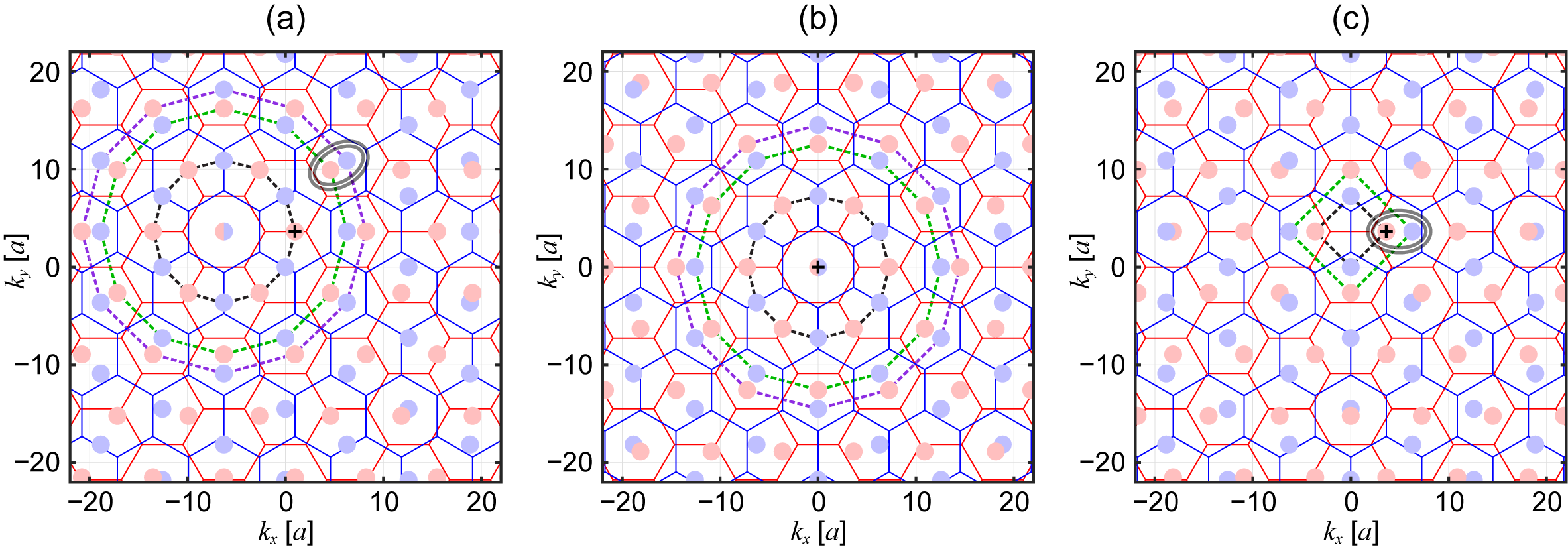
While the discussion in Sec. C.1 is valid for any general CTG, we can obtain further insight on the resonant coupling by visualizing the resonant chains in CTGs with in a dual tight-binding lattice. The subspace spanned by the Hamiltonian of a CTG with from a wave vector is (), where and [Eq. (12)]. According to Eq. (10), the interaction strength between and is given by where . Then, we can visualize the interaction strength by inverting all the wave points and the extended Brillouin zone of the layer with respect to , and overlapping them on those of the layer. Then, the geometric distance between the wave vectors in the two layers, and , represents . Since decays fast as grows, the states located in a closer distance in the map exhibit the stronger interlayer interaction. Thus, if we count each wave vector as a “site”, then the arrangement of the wave vectors of the subspace can be regarded as a tight-binding lattice in the momentum space, which is dual to the original Hamiltonian in the real space [15].
Figure 13(a) shows the dual tight-binding lattice of a CTG with by choosing the of the resonant chain in Fig. 4(a) as (cross mark). The red and blue hexagons show the extended Brillouin zones of the layer and 1, respectively, and the red and blue filled circles represent and , respectively. We inverted both the states and the reciprocal lattices of the layer with respect to . The twelve monolayer Bloch states connected by the black dashed lines are degenerate in energy, as we can clearly see from the relative positions of the waves in the Brillouin zone of each layer. And they interact with the same interaction strength , since they are equally spaced in the dual tight-binding lattice. Thus, these states form a resonant chain as we have already shown in Fig. 4(a).
Each element of the resonant chain interacts not only with the elements of the chain but also with the states outside the chain. However, it is obvious that the interaction to the states outside the chain neither lifts the degeneracy of the elements nor breaks the symmetry of the chain. This is because the surrounding of each element of the chain is identical, since all the wave vectors and the extended Brillouin zones in Fig. 13(a) are arranged in a 12-fold screw rotationally symmetric way around the unique center of the dodecagonal lattice, where the centers of the hexagonal Brillouin zones of the two layers coincide. In addition, the monolayer state energies of the states outside the chain are usually different from that of the chain elements. As we can see from the electronic structures of twisted bilayer graphene [4, 6], if two monolayer Bloch states in different layers have quite different energies, their interaction gives nearly decoupled, monolayerlike band dispersion at those wave vectors no matter how large their is. Thus, the resonant interaction most strongly influences the electronic structures, and the interaction to the states outside the chain merely shifts the resonant energies Eqs. (33)-(35) by some, mostly small, constants.
Note that the chain with the black dashed lines is not the only resonant chain that appears in the map of Fig. 13(a). There are infinitely many resonant chains that satisfy the 12-fold screw rotational symmetry around the center of rotation, regardless of whether the interaction is strong or weak. For example, the monolayer Bloch states connected by the green and purple dashed lines also form distinct resonant chains. A careful look at the difference between the original extended Brillouin zone in Fig. 4 and the inverted Brillouin zone in Fig. 13, we can see that these resonant states are exactly what we have shown in Figs. 4(c) and (d), respectively. The distance between the elements in each of these chains is longer than that in the chain with the black dashed lines, which is consistent with the fact that the chains in Figs. 4(c) and (d) have weaker than the chain in Fig. 4(a). Interestingly, these green and purple resonant chains interact rather strongly with each other, since the distance between the states of the two chains (encircled by a gray line) is much shorter than the distance between the states within each chain. Thus, the “coupled sites” interact with each other and make up the hybrid resonant chains. However, since their monolayer state energies are very different, the coupling merely shifts the resonant energies by small constants. Note that there might be a configuration where the monolayer state forming the resonant chain is accidentally degenerate with either state outside the resonant chain. In that case, the two states form a coupled state, and the twelve symmetric coupled states form a resonant states.
Also note that the used in Fig. 13(a) [ of the chain in Fig. 4(a)] is not the only that can reveal the resonant chains with a 12-fold screw rotational symmetry. The simplest example is the mapping with , which we plot in Fig. 13(b). In this configuration, the center of the dodecagonal Brillouin zone lattice appears at , and all the elements of the subspace are arranged in a 12-fold screw rotationally symmetric way around the center. Accordingly, we get the resonant chains exactly the same as those in Fig. 13(a). In general, the subspace spanned by the Hamiltonian [Eq. (12)] from with any and is equivalent to that spanned from . This is because
| (63) |
and
| (64) |
and the sets of the monolayer Bloch states and are equivalent to and , up to the Bloch phase, respectively. Likewise, and form a dual tight-binding lattice which is equivalent to the lattice composed of and , except a finite shift of the entire lattice along the in-plane direction; the former lattice is shifted by from the latter lattice. For example, since the used in Fig. 13(a) is the in Fig. 4(a), and therein, the lattice in Fig. 13(a) is merely shifted from that in Fig. 13(b) by .
Although the infinitely many combinations of the incommensurate and give infinitely many , such do not cover every point in the Brillouin zone. This is because the cardinality of the points in the Brillouin zone is , while that of such is , and . Thus, there are other interactions which are not shown in Figs. 13(a) and (b). Figure 13(c) shows one of such examples. Here, we plot the dual tight-binding lattice by choosing the of the resonant chain in Fig. 4(b), , as . The lattice does not host a dodecagonal center, since and ; instead, it exhibits a 4-fold screw rotational symmetry. We plot the first two strongest resonant interactions having a 4-fold screw rotational symmetry, which correspond to the resonant chains in Figs. 4(b) and (e), by black and green lines, respectively. Again, these two chains also interact with each other (gray line), but such a coupling merely shifts the resonant energies, since their monolayer state energies are very different.
Appendix D Eigenvectors of the resonant states
References
- Geim and Grigorieva [2013] A. K. Geim and I. V. Grigorieva, Van der waals heterostructures, Nature 499, 419 (2013).
- Wang and Grifoni [2005] S. Wang and M. Grifoni, Helicity and electron-correlation effects on transport properties of double-walled carbon nanotubes, Phys. Rev. Lett. 95, 266802 (2005).
- Lopes dos Santos et al. [2007] J. M. B. Lopes dos Santos, N. M. R. Peres, and A. H. Castro Neto, Graphene bilayer with a twist: Electronic structure, Phys. Rev. Lett. 99, 256802 (2007).
- Mele [2010] E. J. Mele, Phys. Rev. B 81, 161405 (2010).
- Bistritzer and MacDonald [2011] R. Bistritzer and A. H. MacDonald, Proc. Natl. Acad. Sci. 108, 12233 (2011).
- Moon and Koshino [2013] P. Moon and M. Koshino, Phys. Rev. B 87, 205404 (2013).
- Koshino [2015] M. Koshino, New J. Phys. 17, 015014 (2015).
- Stampfli [1986] P. Stampfli, Helv. Phys. Acta 59, 1260 (1986).
- Ahn et al. [2018] S. J. Ahn, P. Moon, T.-H. Kim, H.-W. Kim, H.-C. Shin, E. H. Kim, H. W. Cha, S.-J. Kahng, P. Kim, M. Koshino, Y.-W. Son, C.-W. Yang, and J. R. Ahn, Science 361, 782 (2018).
- Suzuki et al. [2019] T. Suzuki, T. Iimori, S. J. Ahn, Y. Zhao, M. Watanabe, J. Xu, M. Fujisawa, T. Kanai, N. Ishii, J. Itatani, et al., ACS Nano 13, 11981 (2019).
- Takesaki et al. [2016] Y. Takesaki, K. Kawahara, H. Hibino, S. Okada, M. Tsuji, and H. Ago, Chemistry of Materials 28, 4583 (2016).
- Yao et al. [2018] W. Yao, E. Wang, C. Bao, Y. Zhang, K. Zhang, K. Bao, C. K. Chan, C. Chen, J. Avila, M. C. Asensio, et al., Proc. Natl. Acad. Sci. 115, 6928 (2018).
- Chen et al. [2016] X.-D. Chen, W. Xin, W.-S. Jiang, Z.-B. Liu, Y. Chen, and J.-G. Tian, Adv. Mater. 28, 2563 (2016).
- Pezzini et al. [2020] S. Pezzini, V. Miseikis, G. Piccinini, S. Forti, S. Pace, R. Engelke, F. Rossella, K. Watanabe, T. Taniguchi, P. Kim, and C. Coletti, Nano Lett. 20, 3313 (2020).
- Moon et al. [2019] P. Moon, M. Koshino, and Y.-W. Son, Phys. Rev. B 99, 165430 (2019).
- Yu et al. [2020] G. Yu, M. I. Katsnelson, and S. Yuan, Phys. Rev. B 102, 045113 (2020).
- Crosse and Moon [2021] J. A. Crosse and P. Moon, Phys. Rev. B 103, 045408 (2021).
- Liu et al. [2019] Y. Liu, J. Wang, S. Kim, H. Sun, F. Yang, Z. Fang, N. Tamura, R. Zhang, X. Song, J. Wen, et al., Helical van der waals crystals with discretized eshelby twist, Nature 570, 358 (2019).
- Cea et al. [2019] T. Cea, N. R. Walet, and F. Guinea, Nano letters 19, 8683 (2019).
- Wu et al. [2020] F. Wu, R.-X. Zhang, and S. Das Sarma, Phys. Rev. Research 2, 022010 (2020).
- Song et al. [2021] Z. Song, X. Sun, and L.-W. Wang, Eshelby-twisted three-dimensional moiré superlattices, Phys. Rev. B 103, 245206 (2021).
- McClure [1969] J. McClure, Carbon 7, 425 (1969).
- Slater and Koster [1954] J. C. Slater and G. F. Koster, Phys. Rev. 94, 1498 (1954).
- Moon and Koshino [2012] P. Moon and M. Koshino, Phys. Rev. B 85, 195458 (2012).
- [25] Note that the ratio between and of the hexagonal lattices used in this work is different from that used in the previous works ( and ) on the twisted bilayer graphene [26, 6, 9] and graphene on hexagonal boron nitride [31]. In this work, we scaled by a factor of , while keeping , to compensate the deviation of the Fermi velocity of a pristine graphene due to the summation over sites in the hopping range and make the band dispersion and the energies of the van Hove singularities consistent with the experimental results [9, 12].
- Trambly de Laissardière et al. [2010] G. Trambly de Laissardière, D. Mayou, and L. Magaud, Nano Lett. 10, 804 (2010).
- Aubry and André [1980] S. Aubry and G. André, Ann. Israel Phys. Soc 3, 18 (1980).
- Gardner [1977] M. Gardner, Scientific American 236, 110 (1977).
- Levitov [1988] L. S. Levitov, Commun. Math. Phys. 119, 627 (1988).
- Bandres et al. [2016] M. A. Bandres, M. C. Rechtsman, and M. Segev, Phys. Rev. X 6, 011016 (2016).
- Moon and Koshino [2014] P. Moon and M. Koshino, Phys. Rev. B 90, 155406 (2014).