Resolving cosmic star formation histories of present-day bulges, disks, and spheroids with ProFuse
Abstract
We present the first look at star formation histories of galaxy components using ProFuse, a new technique to model the 2D distribution of light across multiple wavelengths using simultaneous spectral and spatial fitting of purely imaging data. We present a number of methods to classify galaxies structurally/morphologically, showing the similarities and discrepancies between these schemes. We show the variation in component-wise mass functions that can occur simply due to the use of a different classification method, which is most dramatic in separating bulges and spheroids. Rather than identifying the best-performing scheme, we use the spread of classifications to quantify uncertainty in our results. We study the cosmic star formation history (CSFH), forensically derived using ProFuse with a sample of 7,000 galaxies from the Galaxy And Mass Assembly (GAMA) survey. Remarkably, the forensic CSFH recovered via both our method (ProFuse) and traditional SED fitting (ProSpect) are not only exactly consistent with each other over the past 8 Gyr, but also with the in-situ CSFH measured using ProSpect. Furthermore, we separate the CSFH by contributions from spheroids, bulges and disks. While the vast majority (70%) of present-day star formation takes place in the disk population, we show that 50% of the stars that formed at cosmic noon (8-12 Gyr ago) now reside in spheroids, and present-day bulges are composed of stars that were primarily formed in the very early Universe, with half their stars already formed 12 Gyr ago.
keywords:
galaxies: bulges – galaxies: elliptical and lenticular, cD – galaxies: evolution – galaxies: general – galaxies: luminosity function, mass function – galaxies: spiral – galaxies: star formation – galaxies: structure1 Introduction
The extraordinary diversity of the present-day galaxy population is marked by a wide variety of galaxy properties. One such property is the physical structure of galaxies, in terms of galaxies that are disk-like in structure, spheroid-like, or the large population that contains multiple structural components.
The build-up of structure in the very early Universe (prior to cosmic noon) is extremely chaotic, with the infall of gas causing immense star formation in large clumps, and lots of galaxy mergers making the definition of galaxy structure difficult (as demonstrated by, for example, Lotz et al., 2004; Elmegreen et al., 2005; Lee et al., 2013). By cosmic noon, however, structure is sufficiently well defined to describe galaxies in the context of substructures such as bulges and disks. As an example, Hashemizadeh et al. (2021) presented visual classifications of galaxies out to , beyond which the fraction of structurally chaotic galaxies increases. From this point, there is an array of physical mechanisms that can result in the transformation and growth of structure with time. Disks can grow a bulge with time, either via disk instabilities funnelling disk material into a central bulge concentration (a structure often referred to as a pseudobulge, Kormendy & Kennicutt 2004), or through mergers that add material straight into a bulge (for example Barsanti et al., 2022). Such a merger-origin bulge is frequently referred to as a “classical” bulge. This two-phase mode is frequently implemented in semi-analytic models to grow bulges (see for example Stevens et al., 2016; Lagos et al., 2018b; Huško et al., 2023). Spheroidal galaxies can be formed from either disk or two-component systems via larger mergers that destroy all existing structure (as demonstrated using the Horizon-AGN simulations by Martin et al., 2018). Potentially, spheroidal systems could rebuild a disk through the accretion of gas, whose angular momentum creates star formation in a disk-like structure (predicted to occur in simulations by Steinmetz & Navarro 2002, and evidence for which is potentially seen in studies by Moffett et al. 2012; Fabricius et al. 2014). Finally, galaxies may experience no morphological change with time, with components instead growing through mechanisms like star formation (the case for disks), or via stellar mass build-up from mergers (usually for spheroidal-like structures, as is the case for the mass growth in brightest cluster galaxies since Bellstedt et al. 2016; Montenegro-Taborda et al. 2023).
These galaxy structures/morphologies have been strongly linked to the star formation properties of the galaxies themselves. This was originally inferred very simply through a strong link between galaxy colour and its shape (for example Driver et al., 2006, who demonstrated that more concentrated galaxies had redder colours), and then through measurements of the star formation rates as well (like Lee et al., 2013). By analysing the galaxy components themselves rather than simply characterising the overall galaxy shape, it was observed that the bulge fraction was also linked to the overall star formation (see for example Fisher et al., 2009; Guo et al., 2015). This led to significant discussion and debate as to the impact of structural components like bulges on the overall star formation in galaxies (for example Martig et al., 2009; Bluck et al., 2014; Cook et al., 2020). Understanding the structural evolution of galaxies in the context of their star formation is therefore needed to build a more consistent picture of galaxy evolution.
Pinpointing not only which evolutionary pathways have occurred across cosmic time, but also in what relative fractions, is an ongoing challenge in the field of galaxy evolution (for example Casteels et al., 2014; Robotham et al., 2014; Bellstedt et al., 2017; Davies et al., 2022). Making progress on this question observationally is hindered by a number of factors, the major one being that we are limited to observing individual galaxies in only a single snapshot. Given this limitation, two separate approaches must be taken to actually infer the temporal evolution of structure. The first of these is to compare galaxy populations across different epochs, to see how they are changing. This approach is relied upon across the field of galaxy evolution to infer the evolution of most properties, including star formation rates (Driver et al., 2018; Thorne et al., 2021), metallicities (Ly et al., 2016; Sanders et al., 2021), velocity dispersion (Wisnioski et al., 2015), velocity profile shapes (Tiley et al., 2019), mass density profiles (Derkenne et al., 2021), and a multitude of other properties, as well as the structure of galaxies (as analysed by Hashemizadeh et al., 2021). There are significant challenges in inferring evolution from different properties though, originating from progenitor bias (just because populations at different epochs have similar mass distributions, does not mean one is the progenitor of the other, as commented by van Dokkum & Franx, 1996; Kaviraj et al., 2009), selection effects, and observational limits. The other approach in inferring temporal evolution is to study the forensic histories of nearby galaxies themselves. What evidence is there in individual galaxies of evolving properties with time?
This two-pronged “in-situ” versus “forensic” approach has been well demonstrated in the pursuit of accurately constraining the cosmic star formation history (CSFH). The now-famous review by Madau & Dickinson (2014) brought together a suite of observational star formation rate density (SFRD) measurements across a wide redshift range to present a CSFH that showed the decline in star formation in the Universe since “cosmic noon” at . The exact nature of the CSFH prior to cosmic noon is still under debate, in particular because characterising the obscuration of star formation due to dust at high- is challenging (for example Kistler et al., 2009; Bourne et al., 2017; Khusanova et al., 2020; Bouwens et al., 2023; Harikane et al., 2023). The alternate mechanism of deriving the CSFH comes from a forensic analysis of a volume-complete sample of low-redshift galaxies. By deriving the star formation histories (SFH) of all galaxies within a volume of the Universe, the CSFH as a whole can be inferred. Stellar populations analysis techniques like SED modelling are usually employed to derive such star formation histories. To reliably construct the CSFH though, it is critical that any age-related degeneracies (such as the well-known age–metallicity degeneracy) are very carefully considered, so that no biases are introduced (see Conroy 2013 for an overview of the general challenges faced when conducting SED fitting). In typical SED fitting implementations, metallicity is assumed to simply be constant over time, where at best this constant value is allowed to be free (as employed in Leja et al., 2017; Carnall et al., 2018; Iyer et al., 2019; Johnson et al., 2021), but at worst it is fixed to a single value (typically solar, for example Yang et al., 2022; Paspaliaris et al., 2023). Such limitations make it challenging (or impossible) to accurately derive the CSFH in this manner, as the derived CSFH peak is then offset from the observationally measured one due to the introduced biases (for example leja2019; Carnall et al., 2019). Recent implementations of more physical approaches to metallicity evolution in SED fitting in the code ProSpect (Robotham et al., 2020) have reduced these age–metallicity related biases, making it much more feasible to reliably reconstruct the CSFH from SED fitting (as demonstrated for the first time using SED fitting by Bellstedt et al., 2020b).
By applying this forensic-style approach not only to galaxies as a whole, but to their structural subcomponents, it is possible to study when the stars in different galaxy structures formed. Actually isolating the stellar populations of galaxy components from imaging has historically required the successful completion of multiple steps. The first of these, is identifying the structural components of a galaxy through an analysis of the galaxy light profiles — a process known as structural decomposition (first presented in analysis such as de Vaucouleurs, 1958). Galaxy light can either be modelled as a single component (usually with a Sérsic profile Sérsic, 1963), or with two or more components (for example Cook et al., 2019).
Multi-wavelength imaging has also been used to increase the quality of galaxy decompositions, as shown by Häußler et al. (2022), using the galapagos-2 code. Delving even deeper, two-dimensional decompositions can be extracted across multiple wavelengths to generate an SED per component. In a separate step, this can then be modelled with an SED-fitting code to extract forensic properties like star formation histories. Works that have used this approach include for example Dimauro et al. (2018) who applied this to 17,600 galaxies from the CANDELS survey, to produce catalogues of bulge and disk properties. Because of this multi-step approach, such studies are complex and intricate, with potentially limited room for scientific interpretation.
With the recent development of ProFuse (Robotham et al., 2022), it is now possible to conduct image decomposition and SED fitting in a single, self-consistent and physically motivated step. This is quite distinct to similar approaches that have been developed recently to extract bulge and disk stellar populations from IFU data (see Robotham et al. 2022 for a more detailed discussion of these other techniques). In this work, we aim to present the first analysis applying this technique to a volume-limited sample, extracting the cosmic star formation history forensically for bulges, disks, and spheroids directly.
The data used in our analysis are described in Sec. 2, with our ProFuse analysis technique and method described in Sec. 3. We present a detailed discussion of how our structural classifications compare to other methods in Sec. 4, and the results from our analysis are presented in Sec. 5. We discuss implications of our results in Sec. 6, and summarise our conclusions in Sec. 7.
The cosmology assumed throughout this paper is , and (consistent with a Planck 15 cosmology Planck Collaboration et al., 2016).
2 Data
This study utilises the wealth of data from the now-public Galaxy And Mass Assembly (GAMA) survey111http://www.gama-survey.org/ (Driver et al., 2011; Liske et al., 2015; Driver et al., 2022a), which is a galaxy redshift survey conducted on the Anglo Australian Telescope covering 250 square degrees, with a total of 303,542 redshifts (Driver et al., 2022a). We focus on a sample of 6,664 galaxies from the three equatorial regions of the GAMA survey (G09, G12, and G15) with high-quality redshift measurements, analysed in Bellstedt et al. (2020b) and also Robotham et al. (2022).
We use multi-wavelength imaging from the GAMA DR4 (Driver et al., 2022a), as outlined by Bellstedt et al. (2020a) in the //////// bands. In the optical bands, the imaging originates from the VST (VLT Survey Telescope, Arnaboldi et al., 1998), collected through the KiDS survey (Kilo Degree Survey, de Jong et al., 2013), and in the infrared the imaging originated from VISTA (Visible and Infrared Survey Telescope for Astronomy, Emerson et al., 2006; Dalton et al., 2006), collected through VIKING (VISTA Kilo-degree INfrared Galaxy survey, Edge et al., 2013). This imaging is all aligned using SWarp (Bertin, 2010) to a common pixel scale of 0.339 arcseconds (matching the native pixel scale of the VISTA image, for further details on this process see Bellstedt et al. 2020a).
Sources in our sample generally have at least 200 pixels of imaging data within the source segment (up to 50,000), demonstrating that in this redshift range we have sufficient 2D resolution elements for our spatial analysis. Futhermore, the imaging is sufficiently deep to ensure detections in all bands. As shown in figure 18 of Bellstedt et al. (2020a), the 5 surface brightness limit of the imaging data range between 22.5 to 25 mag depending on the band, which is substantially deeper than the galaxies in this sample.
To conduct various completeness corrections related to the use of a volume-limited sample throughout this work, we make use of ProSpect-derived values, which estimate the redshift to which any given galaxy is observable given the GAMA DR4 95% completeness limit of (Driver et al., 2022b). These were derived by generating the best-fitting SED for each galaxy (as derived by the ProSpect fits from Bellstedt et al. 2020b using the updated photometry presented by Bellstedt et al. 2020a), and then regenerating this SED at a range of redshifts, identifying the value at which the magnitude limit is reached. Given the unmasked area of 169.29 square degrees covered by the sample in this work, the value can then be converted to a , to represent the fraction of the observed volume within which the galaxy is observable.
3 Method
3.1 ProFuse
The tool that we use to conduct the simultaneous spectral and photometric decomposition of our sources is ProFuse (Robotham et al., 2022). This combines the SED-fitting capabilities of ProSpect Robotham et al. (2020), the structural modelling capabilities of ProFit (Robotham et al., 2017), and the source-finding capabilities of ProFound (Robotham et al., 2018). While ProFuse as a tool in its entirety is relatively new, it has been developed over many years, through the gradual creation and application of its individual building blocks.
The first of these tools was ProFit (Robotham et al., 2017), which was developed to facilitate light profile fitting of galaxies in a generative, Bayesian manner. Previous codes had been prone to model error, making 2D light modelling of large samples of galaxies unwieldy, and the Bayesian nature of ProFit improved this behaviour. ProFit was wielded by studies such as Cook et al. (2019) and Cook et al. (2020) to assess the impact of galaxy bulges in xGASS (Catinella et al., 2010) on the scatter of HI scaling relations and the star forming main sequence, and later by Hashemizadeh et al. (2022) to study the evolution of bulges and disks through cosmic time in the DEVILS survey (Davies et al., 2018).
Separately to ProFit, there was a need to develop a generative and Bayesian tool that was capable of conducting SED fitting in a flexible and physically motivated manner. This inspired the development of ProSpect (Robotham et al., 2020). With a particular desire to flexibly extract unbiased star formation histories (which in turn would ensure more accurate properties such as total stellar mass), ProSpect was applied to a volume-limited sample by Bellstedt et al. (2020b), where the capacity for this code to forensically reconstruct the cosmic star formation history was demonstrated. This was only possible due to the physically motivated implementation of metallicity evolution within ProSpect, shown to realistically evolve metals in galaxies as demonstrated by the correct inferred evolution of the mass–metallicity relation (Bellstedt et al., 2021). This SED fitting tool was soon shown to work just as effectively at higher redshifts using the DEVILS survey by Thorne et al. (2021), with the link between metallicity and star formation histories explored by Thorne et al. (2022b). These studies demonstrated that ProSpect could self-consistently model the local Universe and infer the correct evolution of stellar mass, star formation rate and metallicity. This is as yet undemonstrated by other SED fitting codes, of which numerous exist with various degrees of similarity, e.g Prospector (Leja et al., 2017; Johnson et al., 2021), BAGPIPES (Carnall et al., 2018), MAGPHYS (da Cunha et al., 2008), CIGALE (Noll et al., 2009; Boquien et al., 2019), and BEAGLE (Chevallard & Charlot, 2016) (see Thorne et al. 2021 for a direct comparison of their utility and capabilities). This physically motivated implementation lends itself incredibly well to the incorporation of additional phenomena, as shown through the inclusion of an AGN component by Thorne et al. (2022a), which was even extended to include radio data in the fitting process (Thorne et al., 2023). Through application of this self-consistent stellar and AGN modelling, the link between star formation and AGN activity over 12.5 Gyr of cosmic time could be studied using GAMA and DEVILS by D’Silva et al. (2023).
The final implement in the ProFuse toolbag is a source detection routine, capable of identifying and isolating the flux of the source object, but also nearby stars to facilitate a local extraction of the image point spread function (PSF). This source extraction software is ProFound (Robotham et al., 2018), which has been readily used since its development to extract photometry of large, multi-wavelength imaging datasets for surveys (Bellstedt et al., 2020a; Davies et al., 2021).
While ProFuse is described in great detail by Robotham et al. (2022), we describe our implementation of ProFuse in the following sections.
3.1.1 Structural models
Separate structural models have been applied to each galaxy, similar to those used by Robotham et al. (2022). We generally use a Sérsic profile (Sérsic, 1963) to model individual structural components in galaxies. The separate models are:
-
•
BD: Bulge+Disk mode, with an exponential disk component with Sérsic and a circular de Vaucouleurs bulge with ;
-
•
FS: Free Sérsic mode, featuring a single component with a free Sérsic index;
-
•
PD: PSF bulge + Disk mode, where the disk component has Sérsic , however the bulge is modelled by a point source that is convolved with the image PSF (is different in each band).
-
•
DD: Disk + Disk mode, where both disk components have Sérsic , but the axial ratios and position angles of the disks are free. We expect that this is an infrequently preferred model, however may be appropriate in cases with very prominent bars or colour gradients.
The DD run was not presented in Robotham et al. (2022), however as we will show it is the best-selected model for only a small number of sources.
The implementation of a two-component model with a disk and a free-Sérsic bulge was explored, but with the average sizes of bulges (1 kpc) and the resolution of GAMA, the Sérsic index would be poorly constrained (given the quality of sky subtraction and accuracy of the PSF). This poor constraint would add sufficient degeneracy to the fit, and hence for this work we have deemed it more favourable to simply fix the Sérsic index of the bulge in the BD mode. This is consistent with approaches taken in the literature (for example Simard et al., 2011; Barsanti et al., 2021b), although we note this is simpler than studies that fit a free Sérsic index for the bulge (for example Dimauro et al., 2018; Cook et al., 2019; Costantin et al., 2021; Casura et al., 2022; Häußler et al., 2022).
3.1.2 SED-fitting models
To constrain the relative brightness of the two-dimensional models across different wavelengths, an SED for each component is generated, in much the same way as traditional SED fitting.
The SED modelling implementation used for all four ProFuse configurations is near identical, and follows the ProSpect modelling approach used by Bellstedt et al. (2020b) and Bellstedt et al. (2021). In short, a parametric star formation history is implemented, using the massfunc_snorm_trunc parametrisation, i.e. a skewed Normal star formation history with a truncation implemented in the early Universe (forcing the SFR to be 0 at the start of cosmic time). Metallicity is allowed to evolve linearly (meaning that the metallicity growth is mapped directly to the growth in stellar mass of the component, achieved using the Zfunc_massmap_lin parametrisation), with the final gas-phase metallicity for each component modelled as a free parameter. In two-component configurations, the star formation and metallicity histories are therefore entirely independent for each of the components. Because this star formation and metallicity implementation is identical to ProSpect implementations conducted in previous works (see Bellstedt et al., 2020b, 2021; Thorne et al., 2022a, 2023), we refer the reader to those papers for a detailed presentation of the interplay between metallicity and age, noting that the accurate recovery of the cosmic star formation history by Bellstedt et al. (2020b) using this metallicity evolution implementation demonstrated that the ages are not systematically biased due to this degeneracy.
Because far-IR data are not being used in this ProFuse implementation, there is very little constraining power for the various dust parameters specified in ProSpect. For this reason, we fix the dust parameters to typical galaxy values as identified by Thorne et al. (2022a). The exception is the FS configuration, where we allow the tau parameters (relating to dust opacity) to be free (possible due to the smaller number of free parameters). However even in this configuration the alpha parameters (which relate to the dust temperature) are fixed, as they are unconstrainable without far-IR data.
All of the relevant fixed and free parameters, as well as their values and fitting ranges, have been provided for the four model configuration in Tables 1-4. The total number of free parameters is 13 for FS, 16 for BD, 15 for PD, and 18 for DD.
| Parameter | Log | Range/Value | Units |
|---|---|---|---|
| SFH parameters | |||
| mSFR | Yes | [, 3] | |
| mpeak | No | [, ] | Gyr |
| mperiod | Yes | [, 1] | Gyr |
| mskew | No | [, 1] | – |
| Metallicity parameters | |||
| Zfinal | Yes | [, ] | – |
| Dust parameters | |||
| Yes | [, 1] | – | |
| Yes | [, 1] | – | |
| – | 1 | – | |
| – | 3 | – | |
| – | -0.7 | – | |
| – | -0.7 | – | |
| Structural decomposition parameters | |||
| x | No | [x, x] | pix |
| y | No | [y, y] | pix |
| Yes | [, ] | – | |
| axrat | Yes | [-2, 0] | – |
| Re | Yes | [1, (image max)] | pix |
| ang | No | [-180, 360] | deg |
| Parameter | Log | Range/Value | Units |
|---|---|---|---|
| SFH parameters | |||
| disk mSFR | Yes | [, 3] | |
| disk mpeak | No | [, ] | Gyr |
| disk mperiod | Yes | [, 1] | Gyr |
| disk mskew | No | [, 1] | – |
| bulge mSFR | Yes | [, 3] | |
| bulge mpeak | No | [, ] | Gyr |
| bulgek mperiod | Yes | [, 1] | Gyr |
| bulge mskew | No | [, 1] | – |
| Metallicity parameters | |||
| disk Zfinal | Yes | [, ] | – |
| bulge Zfinal | Yes | [, ] | – |
| Dust parameters | |||
| disk | – | 0.63 | – |
| disk | – | 0.16 | – |
| disk | – | 1 | – |
| disk | – | 3 | – |
| disk | – | -0.7 | – |
| disk | – | -0.7 | – |
| bulge | – | 0.63 | – |
| bulge | – | 0 | – |
| bulge | – | 1 | – |
| bulge | – | 3 | – |
| bulge | – | -0.7 | – |
| bulge | – | -0.7 | – |
| Structural decomposition parameters | |||
| x | No | [x, x] | pix |
| y | No | [y, y] | pix |
| disk | – | 1 | – |
| disk Re | Yes | [1, (image max)] | pix |
| disk axrat | Yes | [-2, 0] | – |
| disk ang | No | [-180, 360] | deg |
| bulge | – | 4 | – |
| bulge Re | Yes | [1, (image max)] | pix |
| bulge axrat | – | 1 | – |
| bulge ang | – | 0 | deg |
| Parameter | Log | Range/Value | Units |
|---|---|---|---|
| SFH parameters | |||
| disk mSFR | Yes | [, 3] | |
| disk mpeak | No | [, ] | Gyr |
| disk mperiod | Yes | [, 1] | Gyr |
| disk mskew | No | [, 1] | – |
| bulge mSFR | Yes | [, 3] | |
| bulge mpeak | No | [, ] | Gyr |
| bulge mperiod | Yes | [, 1] | Gyr |
| bulge mskew | No | [, 1] | – |
| Metallicity parameters | |||
| disk Zfinal | Yes | [, ] | – |
| bulge Zfinal | Yes | [, ] | – |
| Dust parameters | |||
| disk | – | 0.63 | – |
| disk | – | 0.16 | – |
| disk | – | 1 | – |
| disk | – | 3 | – |
| disk | – | -0.7 | – |
| disk | – | -0.7 | – |
| bulge | – | 0.63 | – |
| bulge | – | 0 | – |
| bulge | – | 1 | – |
| bulge | – | 3 | – |
| bulge | – | -0.7 | – |
| bulge | – | -0.7 | – |
| Structural decomposition parameters | |||
| x | No | [x, x] | pix |
| y | No | [y, y] | pix |
| disk | – | 1 | – |
| disk Re | Yes | [1, (image max)] | pix |
| disk axrat | Yes | [-2, 0] | – |
| disk ang | No | [-180, 360] | deg |
| Parameter | Log | Range/Value | Units |
|---|---|---|---|
| SFH parameters | |||
| disk 1 mSFR | Yes | [, 3] | |
| disk 1 mpeak | No | [, ] | Gyr |
| disk 1 mperiod | Yes | [, 1] | Gyr |
| disk 1 mskew | No | [, 1] | – |
| disk 2 mSFR | Yes | [, 3] | |
| disk 2 mpeak | No | [, ] | Gyr |
| disk 2 mperiod | Yes | [, 1] | Gyr |
| disk 2 mskew | No | [, 1] | – |
| Metallicity parameters | |||
| disk Zfinal | Yes | [, ] | – |
| bulge Zfinal | Yes | [, ] | – |
| Dust parameters | |||
| disk 1 | – | 0.63 | – |
| disk 1 | – | 0 | – |
| disk 1 | – | 1 | – |
| disk 1 | – | 3 | – |
| disk 1 | – | -0.7 | – |
| disk 1 | – | -0.7 | – |
| disk 2 | – | 0.63 | – |
| disk 2 | – | 0.16 | – |
| disk 2 | – | 1 | – |
| disk 2 | – | 3 | – |
| disk 2 | – | -0.7 | – |
| disk 2 | – | -0.7 | – |
| Structural decomposition parameters | |||
| x | No | [x, x] | pix |
| y | No | [y, y] | pix |
| disk 1 | – | 1 | – |
| disk 1 Re | Yes | [1, (image max)] | pix |
| disk 1 axrat | Yes | [-2, 0] | – |
| disk 1 ang | No | [-180, 360] | deg |
| disk 2 | – | 1 | – |
| disk 2 Re | Yes | [1, (image max)] | pix |
| disk 2 axrat | Yes | [-2, 0] | – |
| disk 2 ang | No | [-180, 360] | deg |
3.1.3 Dominant uncertainty

With a fitting process as intricate as the one employed in this work, there are a number of potential sources of uncertainty. In general, the dominant uncertainty is the limitations of the model, as opposed to the quality of the data. This is shown in Fig. 1, where we show the distribution of reduced values of the sample for the different model configurations. The vast majority of galaxies have a value around 1, indicating a good fit of the model to the data. There is a subtle skewing of galaxies with values greater than 1 though, indicating in this regime that the uncertainty of the fits is dominated by model systematics. While there are galaxies with , these are the galaxies with low SFRs (shown in the middle panel) and lower numbers of pixels (lower panel). We note that a visual inspection of the fits for these galaxies generally shows good fits with little residual features, an indication that the complexity of our models is likely overfitting the data here. Again, this shows that the dominant uncertainty comes from limitations in the model, rather than the data quality. We note that a simple cut based on source magnitude or pixel number does not a priori identify these overfitted galaxies.
3.1.4 Unfitted galaxies
There are 9 galaxies (corresponding to 0.13% of the sample) for which there was no successful ProFuse fit, and these were therefore omitted from all subsequent analysis. Galaxies that have images missing in any bands, or that do not have sufficient nearby stars from which to measure the PSF will fail the default ProFuse pipeline. This leaves a sample of 6,655 galaxies studied in this work.
3.2 Structural nomenclature
It is essential to be explicit about the nomenclature adopted in our work, as the usage of structural terms varies across the literature. The three terms that we adpot are disks, bulges, and spheroids.
Disk terminology is consistent with the common use, describing any flattened, circular structure. Disks can either be one part of a two-component system, or galaxies can be purely disks. Bulge is used to describe the ellipsoidal structure at the centre of a two-component system. Spheroid, in our work, is used to describe the single-component structures that are ellipsoidal. Note that with this usage, bulges are not deemed to be a subset of spheroids (which is how the term is often used in the literature). In this sense, disks, bulges, and spheroids are not treated as overlapping categories, and are instead viewed as “eigenstructures” of galaxies. We note that our spheroids are a much broader class than the “elliptical” galaxy class.
3.3 Model Selection
Regardless of the manner in which a galaxy decomposition is conducted, an essential part of the process is determining which model configuration best describes a galaxy’s two-dimensional distribution of light. This can be the most challenging part of structural decomposition, as in many cases a single-component model can describe the light distribution of a galaxy just as well as a bulge plus disk model. What should then determine the choice? This choice has frequently been made using visual classifications or inspections (such as in component modelling by Gadotti, 2009). While a completely numerical quantifier is desired (to remove subjective visual decisions), this approach has remained elusive (although it has been described at length in works like Hashemizadeh et al., 2021).
Because reliable and purely numerical discriminators remain controversial, visual classifications have remained important in much morphology/structure-based work. As datasets are increasing in size dramatically though, requiring visual inspections of galaxies is becoming increasingly unfeasible. An alternate approach increasingly being used is machine learning, where effectively a computer is trained to quickly and efficiently replicate a visual classification on a very large scale. Many galaxy morphological classifications have been made in this manner (see for example Walmsley et al., 2022; Li et al., 2023; Fang et al., 2023; Tian et al., 2023). At this stage these classifications have not yet readily been used for much in the way of follow-on science, although an exception to this is Cavanagh et al. (2023), who used machine learning morphologies to study the evolution of lenticular galaxies with cosmic time. The benefit from a machine learning approach is that larger sample sizes can be processed. Machine learning morphologies will suffer the same potential biases that any visual classification scheme will, due do its inherently qualitative nature, and because nearly all machine learning classifictions have been trained on visually classified data.
For our work, we apply a numeric quantifier from our ProFuse outputs to quantitatively categorise our sample into bulges, disks, and spheroids. Acknowledging however that any classification scheme (whether numerical or visual) still bears some ambiguity, a key aim of this work is to demonstrate the inherent uncertainties that still accompany any attempt to classify galaxies into structural classes. We therefore also incorporate a number of different visual morphological classifications that have been conducted for this sample of galaxies. These different classification schemes are outlined in the following subsections.
3.3.1 ProFuse numerical model selection
The numerical best model selection is expanded from Robotham et al. (2022). Using the parameters derived from each of the models, simple arguments are used to decide whether one model is clearly more physical (for example, if the B/T is very low, then there is motivation to assume that only a single component is required to model to the galaxy). In cases where clear physical motivation is not found, the Deviation Information Criterion (DIC) (which is smaller in the case of a better fit to the data) is used to determine preferred models.
We represent this selection visually in Fig. 2.

A galaxy is best-fitted by FS if it satisfies any of the following criteria:
1) if spurious bulges are fit using BD, for galaxies with disk-like profiles using FS
2) if negligibly tiny bulges are fit using PD, for galaxies with disk-like profiles using FS
3) if all two-component models show very high bulge fractions
4) if the fitted disk in a BD system is negligibly small, indicating only the bulge component fits the whole galaxy
Then, of the remaining unclassified galaxies, PD is selected if (measured in pixels), ensuring that a PSF bulge is only used if the fitted bulge in BD mode is significant, but smaller than the PSF.
Finally, all remaining galaxies are classified based on the preferred DIC for each of the models (where a lower value indicates a better fit). The criteria for this are as follows. FS is selected if:
BD is selected if:
PD is selected if:
Finally, of the remaining unclassified galaxies, DD is only selected for a small number of objects for which the model is significantly preferred:
All remaining unclassified galaxies are selected to be FS, as the simplest model is assumed to be sufficient if no more complex models are preferred. The non-zero values in the above criteria are chosen to ensure that only models that are significantly preferred according to their DIC are selected for more discrepant models. In the case of the FS selection, this ensures that potential BD sources are not missed (given that FS is selected as the final default regardless, if no other model is significantly preferred). PD and BD are so similar in terms of model complexity that this significance is not as important. The exact value was selected based on visual calibration (as was the case for each of the selection criteria).
The above criteria have been slightly modified from the similar implementation by Robotham et al. (2022), to better catch two-component systems that were being flagged as single-component (based on extensive visual inspection and optimisation). The final DD criterion has been added (as the DD model had not yet been implemented for that work). The values that are different have been indicated using bold font.
This approach results in a purely numerical mechanism of determining the structure of galaxies. In total, 5,016 galaxies were selected as best modelled by FS (free Sérsic), 456 by BD (bulge and disk), 1,166 by PD (PSF bulge and disk), and only 17 by DD (two disks).
For all sources deemed best-described by a single component with a free Sérsic index (FS), it is necessary to make a separate decision on the type of structure that this component is consistent with, be they disk or spheroidal.
For the sake of the structural analysis in this paper, we use the following criteria to classify these structures. If , the structure is a disk. If , the structure is a spheroid. If , the structure is treated as ambiguous.
Here, the ambiguous classification is simply included as an acknowledgement that the exact Sérsic cut used to separate disks and spheroids contributes to the classification uncertainty, and hence throughout the analysis in this work, the ambiguous sources will be used to contribute to the uncertainty measurements of each population.
4 Comparing classification schemes
The literature is littered with different methods of classifying galaxies into classes that describe their structure. To ensure that our results are not dependent on the choice of classification scheme, we include multiple visual classification schemes in the analysis. For the sake of making comparisons between the results derived from such classifications, it is necessary for us to comment on their relative agreement, or disagreement.
4.1 Visual morphological classifications
A visual re-classification of the 6,664 galaxies of this work has been conducted (by SB) into structural classes that are equivalent to those defined by the automatic ProFuse classifications described in the previous section. The classes used in this classification are much broader and simpler than previously-used schemes, and are limited to three categories: disk, spheroid, and two-component galaxies. These have been called “ classes” throughout the paper.
These classes complement visual classifications that have been previously conducted on this sample by Moffett et al. (2016a) (“ Classes” hereafter), sorting the galaxies into their Hubble types. The Hubble classes used are ellipticals (E), S0-Sa, SB0-SBa, Sab-Scd, SBab-SBcd, Sd-Irr, and Little Blue Spheroid (LBS) classes.
As part of GAMA DR4, Driver et al. (2022b) conducted an additional visual classification that was based on the visual structure of these galaxies, rather than the visual morphology. We refer to these classifications as the “ Classes” hereafter. The DR4 classes separate galaxies into pure disks (D), ellipticals (E), compact sources (C), and then two-component systems, either with a compact bulge (cBD), or with a diffuse bulge (dBD). Galaxies that are too difficult to classify due to irregular structure such as from mergers are labelled “hard” (H), or “hard elliptical” (HE). These account for a tiny fraction of the sample, and as such are not significant in this analysis.
When presenting results from visual classification methods throughout this paper, we use properties derived from our ProFuse modelling. When visual classes have described a galaxy as having a single-component fit, we assign the FS properties to the galaxy. When a two-component system has instead been selected, then we can either assign the BD or PD properties to the galaxy. Wherever relevant for the duration of this paper, we present results with both options, to indicate the plausible uncertainty originating from model selection. We highlight that this is the most pessimistic uncertainty, as a likelihood criterion (as used in the automatic ProFuse classes) can be used to isolate the better-fitting description to shrink this uncertainty. This same approach is taken when presenting the bulge and disk properties using the classes.
4.2 Scheme Comparison


We show a comparison between our ProFuse model classifications and the Classes, Classes, and Classes in Fig. 3. The bijective agreement (which combines the fractional occupation of every class along both the row and the column) between the ProFuse classes and each of the visual classifications is shown in Fig. 3. The darker the matrix element is coloured (as indicated by the colourbar), the better the agreement. For each matrix class combination, we plot the – distribution of the subset, coloured by the colour (the relevant subset of the left-hand panel). For each matrix entry, a dashed box indicates regions that we would reasonably expect to be populated if the classification schemes were working perfectly as intended. The fact that the majority of these regions are highly populated generally suggests that the classification schemes are working fairly consistently.
The lower panel of Fig. 3 shows the equivalent matrix comparison, where the individual agreement percentages are shown in each category (showing greater detail than simply the coloured bijective agreement).
These figures are designed to provide insight into the potential differences in the classification schemes, and include an enormous amount of information. Therefore, an exhaustive analysis of each intersection in these comparison matrices is not the aim of this section. Rather, the below subsections summarise some of the major conclusions apparent from this complex comparison.
4.2.1 Classifying disks
The overlap between disks, and single component disks from ProFuse is high, with a bijective agreement value of 57%. The top left box in the lower panel of Fig. 3 shows that 84% of all visually determined disks according to the classes are flagged as disks according to the ProFuse model classifications, however of the ProFuse class disks, 68% are visually classed as disks. Through comparison with the top panel, it can be seen that the ProFuse disks contain a larger portion of higher-mass, redder objects, that have been visually classed as either two-component or spheroid systems, despite all having low Sersíc indices.
The agreement between visual disks from DR4, and single component disks from ProFuse is also high, with a bijective agreement value of 59.6%. Of the 29% of ProFuse disks that are not classed as DR4 disks, the majority of these fall into the dBD category (disk with a diffuse bulge), which makes sense as such two-component systems with non-compact bulges are likely best modelled by a single component in our ProFuse setup (this uncertainty is shown by the fact that DR4 dBD galaxies are fairly evenly divided between ProFuse Disk, 2-comp, and Ambig categories).
The class that is most similar to pure-disk systems is Sd (where there is no prominent bulge), and so it is reassuring to see that the bijective agreement between ProFuse Disk and Sd-Irr galaxies is also high (with a value of 50.3%). It is notable that there is also a substantial overlap between pure disks and Sab-Scd systems (which are deemed to have smaller bulges), albeit smaller (9.6%).
4.2.2 Classifying spheroids and ellipticals
There is overlap between ProFuse spheroids and spheroids, DR4 ellipticals and ellipticals (with bijective agreement values of 16.1%, 19.1% and 17.7% respectively), which is to be expected. The fact that the bijective agreements are so much lower than those of the pure disk populations, suggest that classifying non-disk single-component systems is much more prone to classification uncertainty. Both our ProFuse and spheroidal populations span the full range of both stellar mass and colour, which is contrasted to both visual elliptical classes that tend to only include high-mass, red galaxies. This is an indication thst colour what a much more influential factor in the classification of galaxies according to the and schemes, unlike the structural-only schemes presented in this paper.
We find that when comparing ProFuse and spheroids with the classes, the majority of these low-mass, blue spheroids are either labelled as LBS (little blue spheroid) galaxies, or a small number of Sd-Irr galaxies. When compared with the classes, the low-mass blue spheroids are instead classified as dBD sources, which are regarded as two-component, but without a typical, compact bulge. This shows that our definition of spheroidal is a much broader class than simply the elliptical class. For this reason it is important not to use the “Elliptical” label for our spheroid class.
4.2.3 Classifying two-component systems
ProFuse-classified two-component systems tend to mostly overlap with either cBD or dBD galaxies in the scheme (as should be expected). There is however a smaller fraction of ProFuse-classified two-component systems (23%) that are visually classified as one of the single-component classes (D, E, or C), which is an indication of the automatic versus visual classification error.
In the scheme there is a slight preference for them to overlap with the S0-Sa class (which would make sense given these are disk galaxies with a prominent bulge), however the number of classes that are populated by the ProFuse-classified two-component systems is large. As indicated by the dashed boxes, there are four classes that would be reasonable to expect are two-component systems, namely SBab-SBcd, Sab-Scd, SB0-SBa, and S0-Sa, however 43% of ProFuse-classified two-component systems are classified as either Sd-Irr, E, or LBS, showing that substantial uncertainty remains in the decision to label these sources as either a single- or two-component system (greater than the disagreement between the ProFuse and classifications).
4.2.4 Disagreement in classifications across schemes
Regions that are more darkly shaded, but that do not have a dashed outline, represent regions where the classifications disagree. The vast majority of such regions actually fall within the ProFuse ambig category, which accurately reflects the ambiguous nature of these sources. In the visual classifications of this work, they most closely relate to the visual spheroidal sources, suggesting that the cut used to separate disks and spheroids in the ProFuse classifiers is perhaps skewed slightly further toward disk than suggested by eye. These ambig sources are most closely linked to dBD sources in the DR4 scheme. This suggests that the ProFuse classifications either miss diffuse bulges, or the visual classification is unnecessarily associating a bulge to a single-component system. Because bulges in our current implementation of ProFuse are always modelled as circular (in both the BD and PD models), it is possible that we are missing pseudobulge-style structures that are inherently elongated (as the two-component model may not be preferred in this scenario). A random sample of galaxies in this category is shown in Fig. 4.

Other categories that are perhaps surprisingly populated are the intersection between ProFuse two-component systems and each of the visual disks and spheroids. Random samples of each category are presented in Figs. 5 and 6 respectively. A second component in each image is only subtle, however it is distinctly arguably that they do exist, suggesting that classification fatigue has resulted in these being missed when classifications were conducted by eye. In this scenario, the automatic classification from ProFuse seems to be superior.


4.2.5 Classification approach for subsequent analysis
Our conclusion based on this comparison is that no single classification scheme appears to be objectively superior to the others, and there are benefits and drawbacks to each scheme. For this reason, this work does not aim to provide a new classification that is superior to previous, but rather to use differing (but complementary) classification schemes to bracket the range of classifications, to estimate classification uncertainty. For the remainder of this paper, we will present results using each of the ProFuse, SB and DR4 structural classifications.
Throughout this paper, when we present statistics relating to the visual classes, we show outputs from our ProFuse modelling. For all single-component visual classes (D, C, E, and H/ HE222Note that this category was not included in Fig. 3 simply because they are infrequently selected classes at our redshift range. ) we use the FS ProFuse model, and for all two-component classses (cBD and dBD), we use the typical BD model. It is important to note therefore that the “total” sample properties according to the two classes will therefore vary (even though the sample itself is the same).
5 Results
5.1 Galaxy Fits


An example of full ProFuse outputs can be seen in figure 8 of Robotham et al. (2022), which demonstrates how the SED and 2D fitting elements of this technique come together to produce an accurate model with a wealth of data for an individual galaxy and its structural components.
As a brief demonstration of the galaxy fits achieved our ProFuse implementation in this work, we show three-band (//) thumbnails of the best-fitting model and corresponding residual for a handful of sources in Figs. 7-8 (with a further selection presented in Appendix A). Residuals shown are the absolute residual, highlighting both the negative and positive features. For each galaxy, the image, model and residual thumbnails are identically scaled, to make all visible features directly comparable.
Fig. 7 shows a handful of examples for which the ProFuse model results in little residual flux, largely due to the lack of visual substructures within the galaxies (seen in the right-most column of the figure). Because these galaxies are smaller on the sky, the lower effective resolution likely smooths over any substructure in the galaxies, making them easier to model.
Structure types that have not been explicitly modelled in this work include components such as bars and spiral arms. Galaxies that have very strong bar features are shown in Fig. 8. Here, it is clear in the right column that there is a notable portion of the galaxy light that has not been well modelled by ProFuse. In particular, the bar is clearly visible in the residual images, and the red colour is dramatically different from the blue spiral arms, hinting at very distinct stellar populations within these structures. While we find that the total SED of the galaxy is still well approximated on average by ProFuse (and hence the global properties are not likely to be dramatically affected), the 2D model is non-optimal. It has been shown by Erwin et al. (2021) that a classical bulge plus disk decomposition of a barred galaxy can overestimate the spheroid components by factor of 4-100. Using the SDSS (Sloan Digital Sky Survey, Stoughton et al., 2002), Nair & Abraham (2010) estimate that 26% of galaxies with have bars, which is higher than the results that come from a visual inspection of our colour residuals, in which we identify bars in 9% of our sample in the same magnitude range. The resulting impact of neglecting bars in our fitting therefore has the potential to affect a significant fraction of our sample, although the light fraction of a bar in a galaxy can vary dramatically, so the true impact is difficult to estimate. Interestingly, while the residual structure for the galaxies in Fig. 8 seems to be similar, a mix of models (BD, FS and PD) were selected for the galaxies themselves. This highlights that the presence of a bar does not tend to influence the automatic classifications from ProFuse, as bars are badly modelled by all model configurations in general.
The residual features have a very strong colour signature. This indicates that an SED analysis of the residual features with ProSpect will already be possible with existing ProFuse outputs, allowing the stellar populations of features such as bars and spiral arms to be studied. For regular structures such as bars, it may be possible to include this as extra modelled structures in ProFuse itself, although care would need to be taken that there is sufficient quality in the imaging to constrain these extra free parameters. While it is beyond the scope of this work to conduct such an analysis, we feel it is a natural future extension. Additional samples of galaxies are presented in the same manner in Appendix A, to demonstrate some of the interesting galaxy phenomena that are identifiable from this modelling method.
5.2 Stellar mass distributions

The stellar mass distributions of the full sample, as well as the disk, bulge, and spheroid populations are shown in Fig. 9, for each of the three classification schemes used in this work. While the sample itself is identical in each of the schemes, the overall stellar mass distribution displays minor variation, thanks to the different combinations of ProFuse models that were selected to best describe each galaxy in each scheme. As mentioned in Sec. 4.1, either PD or BD configurations could be assigned to galaxies that were visually deemed to be two-component systems. Rather than attempt assign a better model numerically to each individual galaxy, we conduct the analysis with both, which gives the most pessimistic estimate of the error. The uncertainty ranges in the bulge and two-component disk components in the middle and bottom panels of Fig. 9 are the extremes bounded by the scenarios where either all two-component systems are described by PD, or all two-component systems are described by BD. The use of PD generally results in a lower-mass bulge (because of the limited size that a bulge can have), and conversely the use of BD can produce higher-mass bulges. This is what is responsible for the substantial uncertainty in the bulge mass distribution at the low- and high-mass extremes. From the automatic ProFuse classes, it seems that lower-mass bulges are generally best described by the PD configuration, whereas high-mass bulges are best described by BD.
There are significant differences that demonstrate the fundamentally different approaches used to classify galaxies. The double-peaked distribution of disks separates relatively cleanly between the pure disk and the two-component disk systems. This is true for all three classification schemes, although to different degrees. The classes produce the highest low-mass peak in two-component disks, whereas the classes have the lowest number of low-mass two-component disks (with the ProFuse classes somewhere in the middle). This behaviour is mirrored in the bulge population, with the classes having the most low-mass bulges, the classes the fewest, with the ProFuse classes somewhere in the middle. In general, it seems that the ProFuse classes produce a result that is the compromise between the different visual schemes at play in the and classes.

To compare the overall mass distribution of our sample with previous work, we present the total mass function in Fig. 10. This is compared against the recent mass function from Driver et al. (2022a), and the previous GAMA mass function from Wright et al. (2017). We see that our mass function appears to be shifted slightly towards higher stellar masses than that of both Wright et al. (2017) and Driver et al. (2022a). This is to be expected, given that the ProFuse-derived stellar masses are on average 0.1 dex larger than that of ProSpect (which is where the stellar masses originated from for the Driver et al. 2022a analysis). This offset is shown in fig. 11 of Robotham et al. (2022), with more detailed discussion than we repeat here.
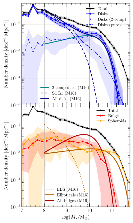
The mass function we derive when dividing by structure types is presented in Fig. 11, where the indicated uncertainty ranges convey the error produced through different classification approaches (compressing the information conveyed in the three panels of Fig. 9). Here, a completeness correction was conducted on a per-galaxy basis using the 1/ values for each galaxy computed using ProSpect. For ease of interpretation, the top panel of Fig. 11 focuses on disk components, whereas the bottom panel focuses on the bulge and spheroid components. We include the Schechter fits to equivalent structure mass functions from Moffett et al. (2016b) in coloured lines. The total disk mass functions are generally consistent, as is the two-component disk distribution. Equivalently, the spheroid distribution is also entirely consistent. Some differences exist when comparing the pure disk systems, where we note that our ProFuse pure disk mass function extends to much higher stellar masses than that of Moffett et al. (2016b). Similarly, our mass function for bulges is much less peaked, and contains a higher density of low-mass bulges than noted by Moffett et al. (2016b).

We present the contribution of bulges, disks, and spheroids to the overall mass budget as a function of stellar mass in Fig. 12, alongside the corresponding curves from Moffett et al. (2016b). It is remarkable that our mass fractions agree well with those measured in the past using Hubble-type classifications alone. At high stellar masses (), our values are indeed entirely consistent. It is just at lower stellar masses where we tend to assign more mass to both bulges and spheroids, and less mass to disks, than Moffett et al. (2016b). Note that LBS objects are not explicitly considered in the curves of Moffett et al. (2016b) (potentially accounting for the difference in the spheroidal populations).
5.3 Cosmic star formation history

Using our volume-limited sample, we derive the star formation rate density (SFRD) with the volume to representing the Universe. The SFRD is derived by summing the star formation histories of all the galaxies in the sample, normalised by the volume. To account for incompleteness at the lowest stellar masses (below ), we scale the contribution of each galaxy to the SFRD by ,333Often referred to simply as a correction to account for the portion of the studied volume over which the galaxy is undetectable within the selection limits. Here, is the volume of the obervational sample, and is the lower between the maximum volume within which the object is observable, or the full volume of the sample.
The resulting total SFRD of our sample derived using our ProFuse method is shown in Fig. 13 as the thick black line. The standard compilation of data points444Measurements included in this compilation come from the following studies: Sanders (2003); Takeuchi et al. (2003); Wyder et al. (2005); Schiminovich et al. (2005); Dahlen et al. (2007); Reddy & Steidel (2009); Robotham & Driver (2011); Magnelli et al. (2011); Magnelli et al. (2013); Cucciati et al. (2012); Bouwens et al. (2012a, b); Schenker et al. (2013); Gruppioni et al. (2013) by Madau & Dickinson (2014) is shown as faint grey data points, as well as the more recent observational measurements of the CSFH by D’Silva et al. (2023).
The forensically derived CSFH using only broadband SED fitting via ProSpect by Bellstedt et al. (2020b)555We present here the SFRD presented in appendix B of Bellstedt et al. (2020b) rather than the main body of the paper, to compare results using the equivalent metallicity evolution prescription. is shown in Fig. 13 as a dashed magenta line. While both this derivation and the in-situ measurement by D’Silva et al. (2023) uses the modelling power of ProSpect, the implemented methods of deriving the SFRD are entirely different. Although the same parametrisation for the SFH and metallicity is used within both ProSpect and ProFuse, the fact that the SFHs can effectively be multi-modal using ProFuse means that these CSFH derivations were by no means destined to look the same. Despite this, the results do agree for the most part, except for slight differences in the early Universe and small discrepancies at low redshift.
This lowest redshift range has been shown in the Fig. 13 inset, highlighted in orange, so that discrepancies are clearer to see. At a lookback time of 1 Gyr, the ProSpect SFRD is larger than that derived by ProFuse by 13% (although the two are still entirely consistent within the uncertainty range introduced by different classification schemes). A possible explanation for the recent dip in the ProFuse CSFH is that star-forming clumps in galaxies (such as in their spiral arms) are not explicitly fitted. This is evident in the residuals shown in Fig. 8. If recent star formation is systematically under-fitted, because the structure is clumpy and not well-described by our model configurations, then we may be systematically underestimating the recent SFR in some cases. An additional contribution to the potential difference at recent times is the manner in which a completeness correction is conducted. A more simplistic correction was conducted by Bellstedt et al. (2020b), which may account for some differences in the lowest lookback time bins of the SFRD.
The other difference between the total CSFH in this work and that derived using ProSpect by Bellstedt et al. (2020b) can be seen at lookback times of greater than 6 Gyr, where the added flexibility of multiple components in this work has resulted in slightly more star formation being recovered (although considering the uncertainties, the discrepancy is only small). Through a comparison of SED-fitting outputs from GAMA, galaxies from the semi-analytic model Shark (Lagos et al., 2018a), and SED-fitted outputs of the Shark galaxies, Bravo et al. (2022) conducted a very thorough analysis to determine the reliability of forensic properties derived from ProSpect. They determined that the evolution of galaxy properties could be accurately reproduced to lookback times of 6 Gyr, but that beyond this epoch, the results start to be dominated by the modelling assumptions. Given that the light from the oldest stellar populations is much fainter than from younger ones, it is unsurprising that the constraint from SED-fitting is much lower here. For this reason, the slight deviation we see in the CSFH between the ProSpect-only and ProFuse derivations may well simply be the consequence of low constraints from these stellar populations. While the absolute SFHs at these older epochs likely have greater uncertainty from SED fitting that limit our derivation of absolute ages, the relative differences between histories for individual populations is still meaningful.
The measurements by D’Silva et al. (2023) are also derived using ProSpect with a linear metallicity evolution model, consistent with the SED modelling approach in this paper. D’Silva et al. (2023) also include AGN in their modelling as described by Thorne et al. (2022a), resulting in an improved estimation of galaxy properties, especially at high-. Our forensic derivation is broadly consistent, however we note that our forensic SFRD is perhaps underestimated in the 8-10 Gyr range, and then overestimated beyond 10 Gyr. The agreement between each of the ProSpect-derived approaches in measuring the SFRD is remarkable within the most recent 8 Gyr of lookback time.

The SFRD with contributions by different components is presented in Fig. 14, with the total SFRD shown in black, and in colour the contributions toward the total SFRD by different galaxy structures, including disks (blue), bulges (red), and spheroids (orange). Values plotted in Fig. 14 are presented in Table 5, with full data available in the supplementary material.
| LbT | Total | Bulge | Bulge (younger) | Bulge (older) | Disk | Pure Disk | 2-comp Disk | Spheroid | |
|---|---|---|---|---|---|---|---|---|---|
| Gyr | |||||||||
| 0.9 | 0.07 | ||||||||
| 1.0 | 0.07 | ||||||||
| 1.1 | 0.08 | ||||||||
| 1.2 | 0.09 | ||||||||
| 1.3 | 0.1 | ||||||||
| … | |||||||||

The corresponding evolution in the stellar mass density inferred by our star formation history is shown in Fig. 15. The impact of the slight difference in total SFRD between ProSpect (from Bellstedt et al. 2020b) and ProFuse is a 16% factor increase in the total stellar mass density. Note that despite this increase, the present-day stellar mass density is still entirely consistent with the compilation data666This compilation includes SMD measurements by Arnouts et al. (2007); Gallazzi et al. (2008); Pérez-González et al. (2008); Kajisawa et al. (2009); Li & White (2009); Marchesini et al. (2009); Yabe et al. (2009); Pozzetti et al. (2010); Caputi et al. (2011); González et al. (2011); Bielby et al. (2012); Lee et al. (2012); Reddy et al. (2012); Ilbert et al. (2013); Labbé et al. (2013); Moustakas et al. (2013); Muzzin et al. (2013) of Madau & Dickinson (2014). Values plotted in Fig. 15 are presented in Table 6, with full data available in the supplementary material.
We discuss the results for each component individually in the following subsections, reiterating that all trends refer to the stars that are within each component at the present day, as opposed to the component that the stars may have been in at previous epochs.
| LbT | Total | Bulge | Bulge (younger) | Bulge (older) | Disk | Pure Disk | 2-comp Disk | Spheroid | |
|---|---|---|---|---|---|---|---|---|---|
| Gyr | |||||||||
| 0.9 | 0.07 | ||||||||
| 1.0 | 0.07 | ||||||||
| 1.1 | 0.08 | ||||||||
| 1.2 | 0.09 | ||||||||
| 1.3 | 0.1 | ||||||||
| … | |||||||||
5.3.1 Cosmic star formation history of disks
Present-day disks are host to the vast majority of stars formed within the last 8 Gyr. We further divide this contribution into that from pure disks, and disks in two-component systems (shown in Fig. 14 and 15 as dashed, and dashed-dotted blue lines respectively). While pure disk systems are responsible for more present-day star formation, this is only very recently true, due to the decline in star formation in two-component disk systems in the past 2 Gyr. The appearance of a recent downturn in the star formation rate density of two-component disks is unlikely to be an indication that bulges cause quenching, and likely simply the consequence of the fact that these disks are more massive, and quenched fractions are greater at higher stellar mass (as discussed in many works, but see for example Peng et al., 2010; Moustakas et al., 2013).
While disks do have some old stars, the fraction of stars from the early Universe () that resides in present-day disks is very small, at only %.
5.3.2 Cosmic star formation history of bulges
Bulges are seen to be a very old population, with the vast majority of stellar mass in present-day bulges already formed by cosmic noon. In fact, half the stars currently in bulges had already been formed by a lookback time of 11.8 Gyrs. These bulge stars are distinctly older than spheroid stars. To confirm that this is not the consequence of dust in highly inclined two-component systems, we compared the bulge CSFH for inclined and face-on systems (based on the axial ratio of the corresponding disk), seeing no bias based on galaxy inclination. This lends confidence that bulges truly are measurably older than spheroids.
It is generally accepted that observationally-identified bulges encompass a range of different physical structures, including “classical” bulges, and also “pseudo-” bulges. These pseudobulges have distinct physical structure (Sandage et al., 1970; Kormendy & Illingworth, 1982; Kormendy & Kennicutt, 2004), and are thought to be younger than their classical counterparts (for example Morelli et al., 2008; Fisher et al., 2009). It is possible that we are missing such pseudobulges in our automatic ProFuse classes of structure, as we do not include a model configuration that has a non-circular bulge with a free Sérsic index. If pseudobulge-hosting galaxies were specified as two-component objects from the visual classifications, however, then a bulge complex would have been forcibly modelled, even if it did not produce the best fit to the imaging data. Therefore, we expect that the stellar populations of these sources would still be represented in the visually identified bulge samples. Any differences between the CSFH derived by the different classification schemes would then be apparent in the uncertainty range presented in Fig. 14. Even considering these uncertainties, bulges are still consistently substantially older than the disk population.
A small subset of the bulges in our analysis are younger than their corresponding disks (8-21%, depending on the classification scheme777Using the ProFuse classifications, this value is 16%.), and so to specifically isolate these bulges from the rest of the population, we show in Fig. 14 the contribution to the bulge CSFH by “normal” older bulges in the red dashed-dotted line, and the contribution by the relatively younger bulges in the red dashed line. The bulges that are relatively younger than their disks, while generally older than the disk population, actually more closely resembles the spheroid stellar populations than the typical bulges. A more detailed analysis of this population, and the potential implications for galaxy formation theories, are left for a future work in which this can be explored in greater depth.
Our results indicate that either young pseudobulges are a very subdominant fraction of the bulge population (as measured by Gadotti 2009 using SDSS), or pseudobulge structures have similar stellar population properties to classical bulges. It is also entirely possible that, because pseudobulges have properties more similar to disks than bulges in terms of bluer stellar populations and lower Sérsic indices, that they have been engulfed by the modelled disks in this analysis. Given the number of -classified dBD sources (visually deemed to have a pseudobulge-like structure) that overlap with the pure disk ProFuse class in Fig. 3, it is reasonable that such sources may have simply been modelled as a single disk. Futhermore it is likely that the BD model applied to pseudobulge sources will have allocated pseudobulge light to the disk component. Our overall bulge fraction may well miss the contribution of such sources. Nonetheless, this suggests that pseudobulges as an entity with stellar populations distinct from either classical bulges or disks are unlikely to be a dominant population. Further investigation is required to discriminate between these scenarios from our modelling. Note as well that our bulge population is quite possibly contaminated by bars (as discussed in Sec. 5.1), which is capable of biasing the bulge CSFH.
5.3.3 Cosmic star formation history of spheroids
The more recent contribution to the CSFH by spheroids is substantially higher than that of bulges. The epoch in which spheroid stars were dominantly formed was cosmic noon (around 9-13 Gyr ago), and while there has been a steady decline in the number of spheroid stars formed since a lookback time of 11 Gyr, spheroids are still responsible for 10-40% of present-day star formation. In fact, the shape of the spheroid SFRD with time very closely resembles that of the total CSFH. This suggests that spheroid population is likely a mixed-bag in terms of SFH properties.
5.4 Future improvements in CSFH measurement
Despite the substantial effort that has been invested in recent years to better constrain the CSFH prior to cosmic noon, there is still significant uncertainty. This is driven by the inherent difficulty in measuring SFRs of galaxies in this epoch, due to uncertainties in the substantial dust corrections required at this epoch (examples of the numerous studies that have attempted to make these measurements using both rest-frame UV and FIR include Kistler et al., 2009; Gruppioni et al., 2013; Bouwens et al., 2015; Rowan-Robinson et al., 2016; Novak et al., 2017; Khusanova et al., 2020, 2021).
The analysis presented in Fig. 13 suggests that the capacity for codes like ProSpect to forensically measure the SFRD is excellent over the last 8 Gyrs. We therefore speculate that in future, one of the most promising methods used to constrain the SFRD will be to conduct a forensic analysis of galaxies at . This is realistically the greatest distance at which forensic-style CSFH extractions are possible, as the stellar mass of the completeness limits becomes too high at greater lookback times, and morphologies become too irregular to model the galaxies well. This is also the epoch at which the uncertainties of the derived stellar mass function increase dramatically in the analysis by Wright et al. (2018). With this forensic approach at higher redshifts, there should then be enough constraining power within high-quality data to access cosmic dawn. The dataset that will make this possible is the complete spectroscopic redshift survey WAVES-deep (Driver et al., 2019) to be conducted on 4MOST (de Jong et al., 2019), and other redshift surveys conducted with facilities like MOONS (Cirasuolo et al., 2020), in combination with high-quality imaging from facilities such as Euclid (Laureijs et al., 2012).
6 Discussion
6.1 Literature comparison of bulge and disk formation epochs
The overall trends presented for bulges, spheroids and disks are qualitatively similar to the parametric model presented by Driver et al. (2013), where star formation in present-day spheroids (referring in that work to all ellipsoidals) was deemed responsible for the bulk of star formation at and before cosmic noon, followed by an increase in star formation in disks. The subtle differences we identify are more prolonged star formation in spheroids, with a slight increase in the fraction of earlier formed stars that end up in present-day disks.
Comparing directly with bulge/disk star formation histories from IFU-based work is difficult, because of the substantially smaller (and incomplete) samples currently studied in that level of detail. The main takeaway from an analysis of lenticular galaxies by Johnston et al. (2022) is that bulges in general seem to be pretty old, but that the spread in ages for disks is much broader (and on average younger than bulges). This is consistent with the picture we see from our complete sample of 7,000 galaxies. Even for individual subsets of galaxies however, a quantitative comparison is hampered by the fundamental differences derived in the star formation histories. For example the difficulty in distinguishing very old populations means that the star formation histories by Johnston et al. (2022) begin at epochs earlier than the start of the Universe. Different stellar populations analysis tools, whether SED fitting tools like ProSpect or spectral fitting tools like ppxf (Cappellari & Emsellem, 2004), will all suffer from similar difficulties in constraining older populations. While there is more information in spectra than broadband photometry, there is also therefore more modelling complexity, and sensitivity to modelling degeneracies and assumptions (for example, ppxf is very sensitive to implementation treatments such as the use of regularization). Given the different approaches used to overcome these challenges, the quantitative histories are not yet directly comparable.
Various observational studies have identified “young” bulges, the existence of which seems to be at odds with our results at first glance. Such young bulge-like structures have been seen at the low-mass end (such as the star-forming nuclear star clusters identified by Johnston et al., 2020), which would not impact the overall bulge CSFH due to the small amount of stellar mass involved. Young star-forming bulges were identified by Barsanti et al. (2021a) in an analysis of cluster galaxies. Such galaxies with bulges younger than disks do exist in our sample (as shown in fig. 21 of Robotham et al., 2022, and discussed in Sec. 5.3.2), however as this only accounts for 12% of the two-component sample, the impact is insufficient to have an overall effect on the mass-weighted bulge CSFH. Nonetheless in Fig. 14 we separate the contribution of these younger bulges, and show that it is distinct to that of the rest of the bulge population.
Recent work by Costantin et al. (2021) applied SED fitting to multi-wavelength photometric decompositions of 156 high- galaxies to study the stellar populations of bulges, disks and spheroids. In their work, a bimodality was identified in the formation epoch of bulges, which contributed to the interpretation by Costantin et al. (2022) of two distinct phases of bulge formation in cosmic time. The bulge SFRD we present in Fig. 14 demonstrates no hint of two distinct phases. Instead, it suggests that bulges are simply a continuously old population, with only a small tail of star formation at recent times (contributed to by the subset of bulges that are younger than their disks). Even when analysing the age distribution of bulges identified in our work (as presented in detail by Robotham et al., 2022), we do not see any clear bimodality. The different redshift epochs studied hamper a direct comparison though, as our forensic approach may not be sensitive to two separate epochs that are both quite old. If so, this suggests that any potential high- bimodality is not reflected in the properties of present-day bulges. Furthermore, the two studies use different SFH parametrisations (Costantin et al. 2021 use a declining delayed exponential parametrisation), which can also contribute to differences in recovered ages.
6.2 The ellipsoidals: spheroids and bulges
As demonstrated by the need to clarify our nomenclature in Sec. 3.2, the physical interpretation of the “ellipsoidal” structures in the Universe (bulges and spheroids) varies across the literature. Are they in fact distinguishable structures with distinct evolutionary pathways (true “eigenstructures”), or are their structural and stellar population properties similar enough to warrant interpretation as a single entity?
Our analysis with ProFuse consistently suggests that spheroids and bulges are distinct populations, whether that be due to distinct size–mass relations as shown by Robotham et al. (2022), the stellar mass distributions, or the overall age of the populations as shown by their distinct contributions to the CSFH888Despite taking care to indicate these CSFH resulting from a range of classification schemes, any contamination of disk-like sources into the spheroidal population could still be influencing the distinction between the bulge and spheroid CSFH. in Fig. 14. This conclusion is similar to that of Gadotti (2009), who finds that high-mass bulges and ellipticals are offset in the size–mass relation, also concluding that they are in fact separate populations999Despite the similar conclusion, the size–mass relation for bulges measured by Robotham et al. (2022) is different to Gadotti (2009).. It is difficult to make clear comparisons, as the spheroidal population that we analyse is a broader population than ellipticals studies by Gadotti. This impact of this is seen when comparing (for example) the spheroid CSFH in Fig. 14 with that of the elliptical CSFH presented in fig. 8 of Bellstedt et al. (2020b), where the elliptical contribution to the CSFH dominates much earlier than the spheroids studies in this work generally. Our spheroids contain a larger portion of younger galaxies with more active star formation, typically at lower stellar masses. In the past, such galaxies have been separated out into distinct classes, such as Kormendy & Bender (2012) who treat elliptical and dwarf elliptical (dE) galaxies as separate classes with distinct luminosity functions (see their fig. 3). This was also presented in the luminosity functions of Binggeli et al. (1988), where elliptical galaxies at the high-luminosity end are held distinct from dE and irregular (Irr) galaxies at the low-luminosity end.
Contrastingly, studies of SMBH-bulge correlations treat ellipticals and bulges not as separate populations, but as a continuous population described collectively as “spheroids” (for example Savorgnan et al., 2016; Savorgnan & Graham, 2016). Ellipsoidals were also treated as a common-origin structure in the simple model by Driver et al. (2013) (also referred to collectively as simply spheroids in that work).
This complexity of interpretation is not clearer in simulations. In analysing the IllustrisTNG simulation, Tacchella et al. (2019) study spheroids and bulges as one continuous class. This is contrasted by Ortega-Martinez et al. (2022), who separate classical bulges and spheroids in their EAGLE-based analysis. Despite separating these populations into categories that seem more consistent with our observational approach, however, the spheroids in their analysis tend to be much more extended, and with a higher Sérsic index, suggesting that this divide is still not quite the same. In semi-analytic models like Galform (Cole et al., 2000) and Shark (Lagos et al., 2018b), pure spheroids aren’t explicitly formed. Instead, bulge-like structures are formed via two main mechanisms: mergers or disk instabilities. For this reason, ellipsoidals in these models are usually divided into disk-instability and merger-origin bulges, which are again different to any other definition of this structure. Yet the labels assigned to these structures are often “pseudobulges” and “classical spheroids” respectively (as applied by Huško et al., 2023), which again makes direct comparisons between studies difficult.
The analysis from this paper, and how it relates to the literature, suggests that finding comparable definitions for disks is relatively straightforward, but that bulges/spheroids are much less clearly defined at this stage. This highlights that our definitions are far from universal, and it is essential that more care is taken in future to characterise the specific elements of the “bulge complex”, to facilitate more direct comparisons.
6.3 Implications for morphological evolution
Our forensic CSFH suggests that around 60% of all stars formed at end up in present-day spheroidal systems, with the other 40% having ended up pretty evenly in both disks and bulges. Because our analysis is a forensic one, it simply reflects which structures stars end up in at the present day, not what type of structures they were formed in. Early results from JWST indicate that substantial morphological evolution has occurred since cosmic noon, with morphological classification of 850 galaxies by Kartaltepe et al. (2023) suggesting that 56% of galaxies at have a visually identifiable disk, with only 38% of galaxies visually identified as spheroids. To really quantify this evolution however, complete studies at high redshift are needed to estimate the mass fraction of each structure, not just the fraction of galaxies that include these structures.
With the quality of imaging now available from JWST, it is possible to conduct bulge/disk decomposition (as Chen et al., 2022, did for a sample of 7 galaxies, demonstrating that a bulge component was already in place for each of them). The contrast between high- measurements and our forensic view of the early Universe clearly indicates that some morphological change must be occurring. The exact mechanism by which this tranformation is occurring is hard to tell from our forensic analysis.
We use the outputs from the semi-analytic model Shark (Lagos et al., 2018a) to further explore the differences between “true” mass fractions of bulges, disks and spheroids with cosmic time, as compared with forensically-derived mass fractions like the ones measured in this work. Seeing how these measurements differ provides some intuition for how better to interpret forensic analyses. This analysis is presented in Fig. 16, where our results from the bottom panel of Fig. 15 are renormalised to show the change in mass fraction for each structural component, relative to the epoch. The absolute fractions of mass in disks and bulges is quite different in Shark to that seen in GAMA, which is quite possibly caused by the tuning of the semi-analytic model. For this reason we do not focus on the absolute fractions, but on the relative build-up of disk and bulge mass, which is more fundamentally linked to the modelled physics. The ProFuse results and the equivalent forensic view from Shark shown as solid lines. The “true” view from Shark is shown as dashed lines.
What the comparison of the true and forensic mass fractions from Shark shows, is that the historical mass in ellipsoidals is likely overestimated with a forensic approach, whereas the historical disk mass is likely underestimated. In the middle panel of Fig. 16, the dark solid line shows the mass fraction in bulges assumed if Shark galaxies were to be analysed forensically, where the age distributions of stars in the present-day structures are analysed (as we have done observationally using ProFuse). This implies that the fraction of mass in bulges was higher at higher lookback times than in the present day (consistent with our forensic measurement). When the relative mass fraction is extracted from Shark by actually measuring this value in-situ at different epochs (shown by the dashed line), it can be seen that the fraction of stars held in bulges is actually relatively constant. This indicates that some of the old stars in present-day bulges must not always have been in a bulge in the past. Given that the reverse trend is shown in the disk component in the bottom panel of Fig. 16, this suggests that it is possible that the old stars forensically attributed to bulges, may have actually come from disks. This points to a morphological evolution pathway, in which stars that are formed in disks likely end up in ellipsoidal structures. This is consistent with the picture of morphological transformation built up based on both observations (for example Dressler, 1980; Hashemizadeh et al., 2022; quilley2022; Marasco et al., 2023) and simulations (for example Bournaud et al., 2007; Clauwens et al., 2018; Martin et al., 2018; Jackson et al., 2019).
We caution that in different semi-analytic models, the “true” picture can differ dramatically to that shown in Shark. For example, Huško et al. (2023) uses Galform to present the fraction of mass in bulges with cosmic time, and these curves differ substantially. In particular, a much lower fraction of mass exists within bulges at the present day, but rises substantially beyond .

7 Conclusions
We have presented here the first star formation history-based analysis to originate from an application of ProFuse, which simultaneously models the two-dimensional structure and SED of the components of galaxies from multiwavelength imaging. The analysis presented has the following, clear conclusions:
- •
-
•
Using the outputs from ProFuse alone through application of multiple structural configurations101010We use a single component with a free Sérsic index (FS), a bulge+disk system (BD), a disk+PSF central component system (PD), or a disk+disk system (DD)., we show that it is possible to automatically define a best-fitting model per individual galaxy. We present the differences in these best models as compared with visual classifications, and discuss the subtleties of any discrepancies. This demonstration shows that we have a pathway for moving beyond visual inspection of galaxies for the purpose of structural classification.
-
•
We showed in this paper that no two classification schemes are fully consistent, and that there are very good reasons why this is the case (most notably that the classification criteria between different schemes vary based on the purpose of the classification, be they morphological, structural, motivated by colours or not, etc). This highlights why literature results based on galaxy decompositions may differ. Rather than justifying why one method is superior to another, we took the approach of using three separate classification schemes, and using the differences to estimate uncertainty in the scientific results. We argue that this provides a fairer estimate of true uncertainties, while also lending greater confidence to the final results.
-
•
Using the star formation histories for individual galaxy components, we measure forensically the cosmic star formation history. Remarkably, the ProFuse CSFH is almost entirely consistent with that derived using global SED fitting of galaxies from ProSpect (Bellstedt et al., 2020b), and also the in-situ measured CSFH from high-z galaxies (Madau & Dickinson, 2014; Driver et al., 2018; D’Silva et al., 2023). In particular, we find that the last 8 Gyr of the CSFH are measured to be perfectly consistent across all methods. This consistency highlights not only that we have an excellent understanding of this fundamental property of our Universe, but also that the techniques we are using to study galaxies are producing consistent results, which is essential in trusting the derived properties themselves.
-
•
Finally, we present the component-wise CSFH, divided by the contributions of present-day disks, bulges, and spheroids. Bulges contain the oldest stars in the Universe, with half of all bulge stars having formed by a lookback time of 11.8 Gyrs. At the present day, a negligible fraction of all star formation occurs in bulges. Disks tell a very different story, accounting for 60-90% of all present-day star formation, with half of disk mass in place by a much later lookback time of 7.9 Gyr. Spheroids are made of stars that have formed relatively consistently with the overall CSFH, being only slightly older than the average stars, with half the mass formed by 10.8 Gyr (as compared with an overall half-mass epoch of 9.9 Gyr). While the age estimate uncertainties of old stars from SED fitting may impact the absolute ages for our sample, we emphasise the relative difference between the populations as meaningful. Spheroids today still account for 10-40% of all star formation, whereas bulges posess almost no star formation in the Universe.
8 Data Availability
The data used as an input to this analysis are all publicly available via the GAMA webpage111111http://www.gama-survey.org. The data presented in this paper can be made available upon reasonable request.
9 Acknowledgements
SB and ASGR acknowledge support from the ARC Future Fellowship scheme (FT200100375). SPD acknowledges support from the ARC Laureate Fellowship scheme (FL220100191). LJWD and RHWC acknowledge support from the ARC Future Fellowship scheme (FT200100055). This work was supported by resources provided by the Pawsey Supercomputing Centre with funding from the Australian Government and the Government of Western Australia.
GAMA is a joint European-Australasian project based around a spectroscopic campaign using the Anglo-Australian Telescope. GAMA was funded by the STFC (UK), the ARC (Australia), the AAO, and the participating institutions. GAMA photometry is based on observations made with ESO Telescopes at the La Silla Paranal Observatory under programme ID 179.A-2004, ID 177.A-3016
We have used R (R Core Team, 2017) and python for our data analysis, and acknowledge the use of Matplotlib (Hunter, 2007) for the generation of plots in this paper. This research made use of the R package celestial (Robotham, 2016), Astropy,121212http://www.astropy.org a community-developed core python package for astronomy (Astropy Collaboration et al., 2013, 2018), Pandas (McKinney, 2010), and NumPy (Harris et al., 2020).
References
- Arnaboldi et al. (1998) Arnaboldi M., Capaccioli M., Mancini D., Rafanelli P., Scaramella R., Sedmak G., Vettolani G. P., 1998, The Messenger, 93, 30
- Arnouts et al. (2007) Arnouts S., et al., 2007, A&A, 476, 137
- Astropy Collaboration et al. (2013) Astropy Collaboration et al., 2013, A&A, 558, A33
- Astropy Collaboration et al. (2018) Astropy Collaboration et al., 2018, AJ, 156, 123
- Barsanti et al. (2021a) Barsanti S., et al., 2021a, ApJ, 906, 100
- Barsanti et al. (2021b) Barsanti S., et al., 2021b, ApJ, 911, 21
- Barsanti et al. (2022) Barsanti S., et al., 2022, MNRAS, 516, 3569
- Bellstedt et al. (2016) Bellstedt S., et al., 2016, MNRAS, 460, 2862
- Bellstedt et al. (2017) Bellstedt S., Forbes D. A., Foster C., Romanowsky A. J., Brodie J. P., Pastorello N., Alabi A., Villaume A., 2017, MNRAS, 467, 4540
- Bellstedt et al. (2020a) Bellstedt S., et al., 2020a, MNRAS, 496, 3235
- Bellstedt et al. (2020b) Bellstedt S., et al., 2020b, MNRAS, 498, 5581
- Bellstedt et al. (2021) Bellstedt S., et al., 2021, MNRAS, 503, 3309
- Bertin (2010) Bertin E., 2010, SWarp: Resampling and Co-adding FITS Images Together
- Bielby et al. (2012) Bielby R., et al., 2012, A&A, 545, A23
- Binggeli et al. (1988) Binggeli B., Sandage A., Tammann G. A., 1988, ARA&A, 26, 509
- Bluck et al. (2014) Bluck A. F. L., Mendel J. T., Ellison S. L., Moreno J., Simard L., Patton D. R., Starkenburg E., 2014, MNRAS, 441, 599
- Boquien et al. (2019) Boquien M., Burgarella D., Roehlly Y., Buat V., Ciesla L., Corre D., Inoue A. K., Salas H., 2019, A&A, 622, A103
- Bournaud et al. (2007) Bournaud F., Jog C. J., Combes F., 2007, Astronomy and Astrophysics, 476, 1179
- Bourne et al. (2017) Bourne N., et al., 2017, MNRAS, 467, 1360
- Bouwens et al. (2012a) Bouwens R. J., et al., 2012a, ApJL, 752, L5
- Bouwens et al. (2012b) Bouwens R. J., et al., 2012b, ApJ, 754, 83
- Bouwens et al. (2015) Bouwens R. J., et al., 2015, ApJ, 803, 34
- Bouwens et al. (2023) Bouwens R., Illingworth G., Oesch P., Stefanon M., Naidu R., van Leeuwen I., Magee D., 2023, MNRAS
- Bravo et al. (2022) Bravo M., Robotham A. S. G., Lagos C. d. P., Davies L. J. M., Bellstedt S., Thorne J. E., 2022, MNRAS, 511, 5405
- Cappellari & Emsellem (2004) Cappellari M., Emsellem E., 2004, PASP, 116, 138
- Caputi et al. (2011) Caputi K. I., Cirasuolo M., Dunlop J. S., McLure R. J., Farrah D., Almaini O., 2011, MNRAS, 413, 162
- Carnall et al. (2018) Carnall A. C., McLure R. J., Dunlop J. S., Davé R., 2018, MNRAS, 480, 4379
- Carnall et al. (2019) Carnall A. C., Leja J., Johnson B. D., McLure R. J., Dunlop J. S., Conroy C., 2019, ApJ, 873, 44
- Casteels et al. (2014) Casteels K. R. V., et al., 2014, MNRAS, 445, 1157
- Casura et al. (2022) Casura S., et al., 2022, MNRAS, 516, 942
- Catinella et al. (2010) Catinella B., et al., 2010, MNRAS, 403, 683
- Cavanagh et al. (2023) Cavanagh M. K., Bekki K., Groves B. A., 2023, MNRAS, 520, 5885
- Chen et al. (2022) Chen C.-C., et al., 2022, ApJ, 939, L7
- Chevallard & Charlot (2016) Chevallard J., Charlot S., 2016, MNRAS, 462, 1415
- Cirasuolo et al. (2020) Cirasuolo M., et al., 2020, The Messenger, 180, 10
- Clauwens et al. (2018) Clauwens B., Schaye J., Franx M., Bower R. G., 2018, MNRAS, 478, 3994
- Cole et al. (2000) Cole S., Lacey C. G., Baugh C. M., Frenk C. S., 2000, MNRAS, 319, 168
- Conroy (2013) Conroy C., 2013, ARA&A, 51, 393
- Cook et al. (2019) Cook R. H. W., Cortese L., Catinella B., Robotham A., 2019, MNRAS, 490, 4060
- Cook et al. (2020) Cook R. H. W., Cortese L., Catinella B., Robotham A., 2020, MNRAS, 493, 5596
- Costantin et al. (2021) Costantin L., et al., 2021, ApJ, 913, 125
- Costantin et al. (2022) Costantin L., et al., 2022, ApJ, 929, 121
- Cucciati et al. (2012) Cucciati O., et al., 2012, ApJ, 539, A31
- D’Silva et al. (2023) D’Silva J. C. J., et al., 2023, MNRAS, 524, 1448
- Dahlen et al. (2007) Dahlen T., Mobasher B., Dickinson M., Ferguson H. C., Giavalisco M., Kretchmer C., Ravindranath S., 2007, ApJ, 654, 172
- Dalton et al. (2006) Dalton G. B., et al., 2006, (SPIE) Conference Series, 6269, 62690X
- Davies et al. (2018) Davies L. J. M., et al., 2018, MNRAS, 480, 768
- Davies et al. (2021) Davies L. J. M., et al., 2021, MNRAS, 506, 256
- Davies et al. (2022) Davies L. J. M., et al., 2022, MNRAS, 509, 4392
- Derkenne et al. (2021) Derkenne C., McDermid R. M., Poci A., Remus R.-S., Jørgensen I., Emsellem E., 2021, MNRAS, 506, 3691
- Dimauro et al. (2018) Dimauro P., et al., 2018, MNRAS, 478, 5410
- Dressler (1980) Dressler A., 1980, ApJ, 236, 351
- Driver et al. (2006) Driver S. P., et al., 2006, MNRAS, 368, 414
- Driver et al. (2011) Driver S. P., et al., 2011, MNRAS, 413, 971
- Driver et al. (2013) Driver S. P., Robotham A. S. G., Bland-Hawthorn J., Brown M., Hopkins A., Liske J., Phillipps S., Wilkins S., 2013, MNRAS, 430, 2622
- Driver et al. (2018) Driver S. P., et al., 2018, MNRAS, 475, 2891
- Driver et al. (2019) Driver S. P., et al., 2019, The Messenger, 175, 46
- Driver et al. (2022a) Driver S. P., et al., 2022a, MNRAS, 513, 439
- Driver et al. (2022b) Driver S. P., et al., 2022b, MNRAS, 515, 2138
- Edge et al. (2013) Edge A., Sutherland W., Kuijken K., Driver S., McMahon R., Eales S., Emerson J. P., 2013, The Messenger, 154, 32
- Elmegreen et al. (2005) Elmegreen D. M., Elmegreen B. G., Rubin D. S., Schaffer M. A., 2005, ApJ, 631, 85
- Emerson et al. (2006) Emerson J., McPherson A., Sutherland W., 2006, The Messenger, 126, 41
- Erwin et al. (2021) Erwin P., et al., 2021, MNRAS, 502, 2446
- Fabricius et al. (2014) Fabricius M. H., et al., 2014, MNRAS, 441, 2212
- Fang et al. (2023) Fang G., et al., 2023, AJ, 165, 35
- Fisher et al. (2009) Fisher D. B., Drory N., Fabricius M. H., 2009, ApJ, 697, 630
- Gadotti (2009) Gadotti D. A., 2009, MNRAS, 393, 1531
- Gallazzi et al. (2008) Gallazzi A., Brinchmann J., Charlot S., White S. D. M., 2008, MNRAS, 383, 1439
- González et al. (2011) González V., Labbé I., Bouwens R. J., Illingworth G., Franx M., Kriek M., 2011, ApJL, 735, L34
- Gruppioni et al. (2013) Gruppioni C., et al., 2013, MNRAS, 432, 23
- Guo et al. (2015) Guo K., Zheng X. Z., Wang T., Fu H., 2015, ApJL, 808, L49
- Harikane et al. (2023) Harikane Y., Nakajima K., Ouchi M., Umeda H., Isobe Y., Ono Y., Xu Y., Zhang Y., 2023, Pure Spectroscopic Constraints on UV Luminosity Functions and Cosmic Star Formation History From 25 Galaxies at $z_\mathrm{spec}=8.61-13.20$ Confirmed with JWST/NIRSpec, doi:10.48550/arXiv.2304.06658
- Harris et al. (2020) Harris C. R., et al., 2020, Nature, 585, 357
- Hashemizadeh et al. (2021) Hashemizadeh A., et al., 2021, MNRAS, 505, 136
- Hashemizadeh et al. (2022) Hashemizadeh A., et al., 2022, MNRAS, 515, 1175
- Häußler et al. (2022) Häußler B., et al., 2022, A&A, 664, A92
- Hunter (2007) Hunter J. D., 2007, Computing in Science and Engineering, 9, 90
- Huško et al. (2023) Huško F., Lacey C. G., Baugh C. M., 2023, MNRAS, 518, 5323
- Ilbert et al. (2013) Ilbert O., et al., 2013, A&A, 556, A55
- Iyer et al. (2019) Iyer K. G., Gawiser E., Faber S. M., Ferguson H. C., Kartaltepe J., Koekemoer A. M., Pacifici C., Somerville R. S., 2019, ApJ, 879, 116
- Jackson et al. (2019) Jackson R. A., Martin G., Kaviraj S., Laigle C., Devriendt J. E. G., Dubois Y., Pichon C., 2019, MNRAS, 489, 4679
- Johnson et al. (2021) Johnson B. D., Leja J., Conroy C., Speagle J. S., 2021, ApJSS, 254, 22
- Johnston et al. (2020) Johnston E. J., et al., 2020, MNRAS, 495, 2247
- Johnston et al. (2022) Johnston E. J., et al., 2022, MNRAS, 514, 6141
- Kajisawa et al. (2009) Kajisawa M., et al., 2009, ApJ, 702, 1393
- Kartaltepe et al. (2023) Kartaltepe J. S., et al., 2023, ApJ, 946, L15
- Kaviraj et al. (2009) Kaviraj S., Devriendt J. E. G., Ferreras I., Yi S. K., Silk J., 2009, A&A, 503, 445
- Khusanova et al. (2020) Khusanova Y., et al., 2020, A&A, 634, A97
- Khusanova et al. (2021) Khusanova Y., et al., 2021, A&A, 649, A152
- Kistler et al. (2009) Kistler M. D., Yüksel H., Beacom J. F., Hopkins A. M., Wyithe J. S. B., 2009, ApJL, 705, L104
- Kormendy & Bender (2012) Kormendy J., Bender R., 2012, ApJSS, 198, 2
- Kormendy & Illingworth (1982) Kormendy J., Illingworth G., 1982, ApJ, 256, 460
- Kormendy & Kennicutt (2004) Kormendy J., Kennicutt Jr. R. C., 2004, ARAA, 42, 603
- Labbé et al. (2013) Labbé I., et al., 2013, ApJ, 777, L19
- Lagos et al. (2018a) Lagos C. d. P., et al., 2018a, MNRAS, 473, 4956
- Lagos et al. (2018b) Lagos C. d. P., Tobar R. J., Robotham A. S. G., Obreschkow D., Mitchell P. D., Power C., Elahi P. J., 2018b, MNRAS, 481, 3573
- Laureijs et al. (2012) Laureijs R., et al., 2012, Space Telescopes and Instrumentation 2012: Optical, Infrared, and Millimeter Wave, 8442, 84420T
- Lee et al. (2012) Lee K.-S., et al., 2012, ApJ, 752, 66
- Lee et al. (2013) Lee B., et al., 2013, ApJ, 774, 47
- Leja et al. (2017) Leja J., Johnson B. D., Conroy C., van Dokkum P. G., Byler N., 2017, ApJ, 837, 170
- Li & White (2009) Li C., White S. D. M., 2009, MNRAS, 398, 2177
- Li et al. (2023) Li G., Xu T., Li L., Gao X., Liu Z., Cao J., Yang M., Zhou W., 2023, MNRAS, 523, 488
- Liske et al. (2015) Liske J., et al., 2015, MNRAS, 452, 2087
- Lotz et al. (2004) Lotz J. M., Primack J., Madau P., 2004, AJ, 128, 163
- Ly et al. (2016) Ly C., Malkan M. A., Rigby J. R., Nagao T., 2016, ApJ, 828, 67
- Madau & Dickinson (2014) Madau P., Dickinson M., 2014, ARAA, 52, 415
- Magnelli et al. (2011) Magnelli B., Elbaz D., Chary R. R., Dickinson M., Le Borgne D., Frayer D. T., Willmer C. N. A., 2011, ApJ, 528, A35
- Magnelli et al. (2013) Magnelli B., et al., 2013, ApJ, 553, A132
- Marasco et al. (2023) Marasco A., Poggianti B. M., Fritz J., Werle A., Vulcani B., Moretti A., Gullieuszik M., Kulier A., 2023, MNRAS, 525, 5359
- Marchesini et al. (2009) Marchesini D., van Dokkum P. G., Förster Schreiber N. M., Franx M., Labbé I., Wuyts S., 2009, ApJ, 701, 1765
- Martig et al. (2009) Martig M., Bournaud F., Teyssier R., Dekel A., 2009, ApJ, 707, 250
- Martin et al. (2018) Martin G., Kaviraj S., Devriendt J. E. G., Dubois Y., Pichon C., 2018, MNRAS, 480, 2266
- McKinney (2010) McKinney W., 2010, in van der Walt S., Millman J., eds, Proceedings of the 9th Python in Science Conference. pp 51–56
- Moffett et al. (2012) Moffett A. J., Kannappan S. J., Baker A. J., Laine S., 2012, ApJ, 745, 34
- Moffett et al. (2016a) Moffett A. J., et al., 2016a, MNRAS, 457, 1308
- Moffett et al. (2016b) Moffett A. J., et al., 2016b, MNRAS, 462, 4336
- Montenegro-Taborda et al. (2023) Montenegro-Taborda D., Rodriguez-Gomez V., Pillepich A., Avila-Reese V., Sales L. V., Rodríguez-Puebla A., Hernquist L., 2023, MNRAS, 521, 800
- Morelli et al. (2008) Morelli L., et al., 2008, MNRAS, 389, 341
- Moustakas et al. (2013) Moustakas J., et al., 2013, ApJ, 767, 50
- Muzzin et al. (2013) Muzzin A., et al., 2013, ApJ, 777, 18
- Nair & Abraham (2010) Nair P. B., Abraham R. G., 2010, ApJS, 186, 427
- Noll et al. (2009) Noll S., Burgarella D., Giovannoli E., Buat V., Marcillac D., Muñoz-Mateos J. C., 2009, åp, 507, 1793
- Novak et al. (2017) Novak M., et al., 2017, ApJ, 602, A5
- Ortega-Martinez et al. (2022) Ortega-Martinez S., Obreja A., Dominguez-Tenreiro R., Pedrosa S. E., Rosas-Guevara Y., Tissera P. B., 2022, MNRAS, 516, 197
- Paspaliaris et al. (2023) Paspaliaris E.-D., Xilouris E. M., Nersesian A., Bianchi S., Georgantopoulos I., Masoura V. A., Magdis G. E., Plionis M., 2023, A&A, 669, A11
- Peng et al. (2010) Peng Y.-j., et al., 2010, ApJ, 721, 193
- Pérez-González et al. (2008) Pérez-González P. G., et al., 2008, ApJ, 675, 234
- Planck Collaboration et al. (2016) Planck Collaboration et al., 2016, A&A, 594, A13
- Pozzetti et al. (2010) Pozzetti L., et al., 2010, A&A, 523, A13
- R Core Team (2017) R Core Team 2017, R: A Language and Environment for Statistical Computing. R Foundation for Statistical Computing, Vienna, Austria
- Reddy & Steidel (2009) Reddy N. A., Steidel C. C., 2009, ApJ, 692, 778
- Reddy et al. (2012) Reddy N., et al., 2012, ApJ, 744, 154
- Robotham (2016) Robotham A. S. G., 2016, Astrophysics Source Code Library, p. ascl:1602.011
- Robotham & Driver (2011) Robotham A. S. G., Driver S. P., 2011, MNRAS, 413, 2570
- Robotham et al. (2014) Robotham A. S. G., et al., 2014, MNRAS, 444, 3986
- Robotham et al. (2017) Robotham A. S. G., Taranu D. S., Tobar R., Moffett A., Driver S. P., 2017, MNRAS, 466, 1513
- Robotham et al. (2018) Robotham A. S. G., Davies L. J. M., Driver S. P., Koushan S., Taranu D. S., Casura S., Liske J., 2018, MNRAS, 476, 3137
- Robotham et al. (2020) Robotham A. S. G., Bellstedt S., Lagos C. d. P., Thorne J. E., Davies L. J., Driver S. P., Bravo M., 2020, MNRAS, 495, 905
- Robotham et al. (2022) Robotham A. S. G., Bellstedt S., Driver S. P., 2022, MNRAS, 513, 2985
- Rowan-Robinson et al. (2016) Rowan-Robinson M., et al., 2016, MNRAS, 461, 1100
- Sandage et al. (1970) Sandage A., Freeman K. C., Stokes N. R., 1970, ApJ, 160, 831
- Sanders (2003) Sanders R. H., 2003, MNRAS, 342, 901
- Sanders et al. (2021) Sanders R. L., et al., 2021, ApJ, 914, 19
- Savorgnan & Graham (2016) Savorgnan G. A. D., Graham A. W., 2016, ApJ, 222, 10
- Savorgnan et al. (2016) Savorgnan G. A. D., Graham A. W., Marconi A., Sani E., 2016, ApJ, 817, 21
- Schenker et al. (2013) Schenker M. A., et al., 2013, ApJ, 768, 196
- Schiminovich et al. (2005) Schiminovich D., et al., 2005, ApJL, 619, L47
- Sérsic (1963) Sérsic J. L., 1963, Boletin de la Asociacion Argentina de Astronomia La Plata Argentina, 6, 41
- Simard et al. (2011) Simard L., Mendel J. T., Patton D. R., Ellison S. L., McConnachie A. W., 2011, ApJSS, 196, 11
- Steinmetz & Navarro (2002) Steinmetz M., Navarro J. F., 2002, New Astronomy, 7, 155
- Stevens et al. (2016) Stevens A. R. H., Croton D. J., Mutch S. J., 2016, MNRAS, 461, 859
- Stoughton et al. (2002) Stoughton C., et al., 2002, AJ, 123, 485
- Tacchella et al. (2019) Tacchella S., et al., 2019, MNRAS, 487, 5416
- Takeuchi et al. (2003) Takeuchi T. T., Yoshikawa K., Ishii T. T., 2003, ApJL, 587, L89
- Thorne et al. (2021) Thorne J. E., et al., 2021, MNRAS, 505, 540
- Thorne et al. (2022a) Thorne J. E., et al., 2022a, MNRAS, 509, 4940
- Thorne et al. (2022b) Thorne J. E., et al., 2022b, MNRAS, 517, 6035
- Thorne et al. (2023) Thorne J. E., Robotham A. S. G., Bellstedt S., Davies L. J. M., 2023, MNRAS, 522, 6354
- Tian et al. (2023) Tian C., et al., 2023, ApJ, 944, 124
- Tiley et al. (2019) Tiley A. L., et al., 2019, MNRAS, 485, 934
- Walmsley et al. (2022) Walmsley M., et al., 2022, MNRAS, 509, 3966
- Wisnioski et al. (2015) Wisnioski E., et al., 2015, ApJ, 799, 209
- Wright et al. (2017) Wright A. H., et al., 2017, MNRAS, 470, 283
- Wright et al. (2018) Wright A. H., Driver S. P., Robotham A. S. G., 2018, MNRAS, 480, 3491
- Wyder et al. (2005) Wyder T. K., et al., 2005, ApJL, 619, L15
- Yabe et al. (2009) Yabe K., Ohta K., Iwata I., Sawicki M., Tamura N., Akiyama M., Aoki K., 2009, ApJ, 693, 507
- Yang et al. (2022) Yang G., et al., 2022, ApJ, 927, 192
- da Cunha et al. (2008) da Cunha E., Charlot S., Elbaz D., 2008, MNRAS, 388, 1595
- de Jong et al. (2013) de Jong J. T. A., et al., 2013, The Messenger, 154, 44
- de Jong et al. (2019) de Jong R. S., et al., 2019, The Messenger, 175, 3
- de Vaucouleurs (1958) de Vaucouleurs G., 1958, ApJ, 128, 465
- van Dokkum & Franx (1996) van Dokkum P. G., Franx M., 1996, MNRAS, 281, 985
Appendix A ProFuse individual fitting outputs
In the main body of the text, we presented some examples of the colour images, models and residuals, for a handful of galaxies that have very little residual structure (Fig. 7), and also galaxies that have clear bar structures in their residual (Fig. 8). As a further indication of the wealth of information extractable through these residual visualisations (a task that we will leave for follow-up studies), we have collated a number of examples for different features. Fig. 17 shows examples of galaxies where the different colours of the modelled structural components have created clear colour gradients in the modelled galaxy. When comparing this to the image, this seems to be sensible in most cases.

An additional type of feature identified in the examples shown in Fig. 18, is coloured asymmetry, usually on either side of the galaxy long axis, where one side is noticeably redder than the other. While we do not explore this feature, we suspect it is likely a signature of dust in the galaxy.

Finally, an assortment of miscellanous additional features is presented in Fig. 19. This includes features like very thin disks, rings, and spiral arms. These residuals are generally not an indication of a poor fit, but rather a sign that there is substructure present that has not been accounted for by the four ProFuse model configurations applied in this work.

Appendix B Robustness of fully automated ProFuse classifications
As a demonstration of how well the purely-ProFuse classifications work (as opposed to the visual classification), we show a modified version of Fig. 11 in Fig. 20.
