This paper was converted on www.awesomepapers.org from LaTeX by an anonymous user.
Want to know more? Visit the Converter page.

Resilient Time-Varying Output Formation Tracking of Linear Multi-Agent Systems Against Unbounded FDI Sensor Attacks and Unreliable Digraphs

Zhi Feng and Guoqiang Hu This work was supported by Singapore Ministry of Education Academic Research Fund Tier 1 RG180/17(2017-T1-002-158) and in part by the Wallenberg-NTU Presidential Postdoctoral Fellow Start-Up Grant. Z. Feng and G. Hu are with the School of Electrical and Electronic Engineering, Nanyang Technological University, Singapore 639798 (E-mail: [email protected]; [email protected]).
Abstract

One salient feature of cooperative formation tracking is its distributed nature that relies on localized control and information sharing over a sparse communication network. That is, a distributed control manner could be prone to malicious attacks and unreliable communication that deteriorate the formation tracking performance or even destabilize the whole multi-agent system. This paper studies a safe and reliable time-varying output formation tracking problem of linear multi-agent systems, where an attacker adversely injects any unbounded time-varying signals (false data injection (FDI) attacks), while an interruption of communication channels between the agents is caused by an unreliable network. Both characteristics improve the practical relevance of the problem to be addressed, which poses some technical challenges to the distributed algorithm design and stability analysis. To mitigate the adverse effect, a novel resilient distributed control architecture is established to guarantee time-varying output formation tracking exponentially. The key features of the proposed framework are threefold: 1) an observer-based identifier is integrated to compensate for adverse effects; 2) a reliable distributed algorithm is proposed to deal with time-varying topologies caused by unreliable communication; and 3) in contrast to the existing remedies that deal with attacks as bounded disturbances/faults with known knowledge, we propose resilience strategies to handle unknown and unbounded attacks for exponential convergence of dynamic formation tracking errors, whereas most of existing results achieve uniformly ultimately boundedness (UUB) results. Numerical simulations are given to show the effectiveness of the proposed design.

Index Terms:
Dynamic output formation tracking, Heterogeneous linear multi-agent system, Unbounded attacks, Unreliable digraphs, Resilient distributed control, Global exponential convergence.

I Introduction

Formation control of the multi-agent system has attracted considerable attention in recent years due to its potential applications such as cooperative localization [1], surveillance [2] and moving target enclosing [3]. The main objective of formation control is to present distributed control protocols via neighboring interactions such that the states of all agents can form a desired configuration. In addition to time-invariant formation control, the formation of a team of agents in many practical applications (target enclosing or source seeking) often changes, and is required to track a desired reference. Thus, a time-varying formation tracking problem arises where the agent team can maintain a time-varying formation and meanwhile, track a reference. Based on neighboring interactions, time-varying formation tracking is investigated for homogeneous multi-agent systems with single-/double-integrator [1], high-order linear [5, 4] and nonholonomic [3] dynamics. In practice, each agent has different dynamics and dimensions. That is, the exiting approaches in [1, 2, 3, 5, 4] cannot be directly applied for heterogeneous systems. Recently, formation tracking of heterogeneous systems is studied in [7, 8, 6] via an output regulation scheme.

Notice that all aforementioned works relied on the availability of the local healthy sensors of each agent of the team associated with a reliable communication network. However, the multi-agent systems involving the communication and collaboration between connected agents, are prone to malicious cyber-attacks such as the DoS attacks, deception attacks (FDI attacks or replay attacks), and disclosure attacks [9, 10, 11, 13, 12, 14, 16, 15]. In this paper, we focus on these FDI attacks on the sensors by injecting any false signals to manipulate sensor measurements. Moreover, each agent can communicate via an unreliable network. Note that both characteristics may severely affect the performance of the system, prohibit the accomplishment of system-level objectives, and even destabilize the whole multi-agent system. In light of a wide application of distributed control schemes in a cyber-physical system (safety-critical), and inspired by the studies of security issues in many existing works [9, 10, 11, 13, 12, 14, 16, 15], it is desirable to see if the distributed formation tracking algorithm can provide certain resilience against FDI attacks over unreliable communication. Hence, the objective of this paper is to address a safe and reliable time-varying output formation tracking problem of heterogeneous linear multi-agents to provide certain resilience against unbounded FDI attacks and unreliable communication. So far, this problem is still open, and to the best of our knowledge, few efforts are made on this issue.

This paper investigates resilient time-varying output formation tracking problems of heterogeneous linear multi-agent system in the presence of unbounded FDI attacks and unreliable networks. The resilient distributed estimator-based control algorithms without requiring any attack information, are proposed to deal with the problem over directed topologies caused by unreliable communications. The previous works in [13, 12, 14, 15] studied secure consensus only for homogeneous multi-agent system under DoS attacks. The designs in [9, 10, 11] and [18, 19, 17, 20, 21] to deal with the sensor/actuator attacks or faults highly depended on some assumptions that those attacks or faults either satisfy some special structures or are upper bounded with known knowledge. Those aforementioned works do not consider malicious FDI attacks that are rational, unknown and unbounded. As compared to those works, the main contributions of this paper can be summarized as follows.

  • A resilient distributed estimator-based control framework is developed for heterogeneous linear multi-agent systems with sensor attacks and unreliable digraphs. A reliable distributed leader estimator is firstly proposed to reconstruct the leader’s state for each agent over unreliable communication. Further, a novel resilient distributed output feedback control algorithm is designed to achieve global exponential convergence of the proposed algorithm such that the output of each follower can not only maintain the prescribed time-varying formation, but also track the output of the leader’s trajectory.

  • In contrast to works in [9, 10, 11] in which resilient function calculation and consensus were investigated under the constraints on the number of malicious agents or certain special structure attacks, those requirements are not required in this work. Instead, we only suppose that information interaction over the unreliable communication is allowed to be switching between a graph set containing a directed spanning tree and a paralyzed graph set (in Assumption 1), which is less mild than the fixed undirected or directed graphs in [5, 4, 7, 8, 6, 9, 10, 11].

  • Compared with existing works in [18, 19, 17, 20, 21] to handle attacks or faults as disturbances that have to be bounded with a prior knowledge, the malicious FDI sensor attacks in this work are intelligent, unknown and unbounded, which are practical and reasonable. The proposed scheme does not require any attack information. Moreover, a global exponential convergence can be achieved under attacks, while only the uniformly ultimate boundedness (UUB) result is obtained in [19, 20, 21].

  • The novel resilient distributed output feedback control architecture enables the global exponential stability of the system for time-varying output containment-formation tracking with multiple leaders. Local sufficient conditions and design procedures are presented via the Lyapunov analysis.

The rest of this paper is organized below. The preliminaries and problem formulation are provided in Section II. The resilient time-varying output formation tracking results are proposed in Section III with the global exponential convergence analysis. The design is further extended for resilient time-varying output containment-formation tracking with multiple leaders in Section IV. Examples and numerical simulation results are given in Section V, followed by the conclusion in Section VI.

II Preliminaries and Problem Formulation

II-A Mathematical Preliminaries

Notation: let \mathbb{R}, n\mathbb{R}^{n} and n×m\mathbb{R}^{n\times m} be the sets of the real numbers, real nn-dimensional vectors and real n×mn\times m matrices, respectively. Let >0\mathbb{R}_{>0} be the set of all positive real numbers and \mathbb{N} denote the set of all positive natural numbers. Let 0 (1) be the vector with all zeros (ones) with proper dimensions, respectively. Denote col(x1,,xn)(x_{1},...,x_{n}) and diag{a1,,an}\{a_{1},...,a_{n}\} as a column vector with all entries xix_{i} and a diagonal matrix with all entries aia_{i}, i=1,,ni=1,\cdots,n, respectively. \otimes and \left\|\cdot\right\| are the Kronecker product and Euclidean norm, respectively. Given a real matrix M=MTM=M^{T}, let M>0M>0 be positive definite. Let λmin(M)\lambda_{\min}(M), λmax(M)\lambda_{\max}(M) be its minimum and maximum eigenvalues, respectively. Besides, σmax(M)\sigma_{\max}(M) represents the maximum singular value of a matrix MM.

Graph Theory: Let 𝒢\mathcal{G} == {𝒱,}\left\{\mathcal{V},\mathcal{E}\right\} be a graph and 𝒱\mathcal{V} \in {1,,N}\left\{1,...,N\right\} be the set of vertices. The set of edges is denoted as \mathcal{E} \subseteq 𝒱×𝒱\mathcal{V\times V}. 𝒩i\mathcal{N}_{i} == {j𝒱(j,i)}\left\{j\in\mathcal{V\mid}(j,i)\in\mathcal{E}\right\} is the neighborhood set of vertex ii. For a directed graph 𝒢\mathcal{G}, (i,j)(i,j)\in\mathcal{E} means that the information of node ii is accessible to node jj, but not conversely. The matrix 𝒜=[aij]\mathcal{A}=\left[a_{ij}\right] denotes the adjacency matrix of 𝒢\mathcal{G}, where aij>0a_{ij}>0 if (j,i)(j,i)\in\mathcal{E}, else aij=0a_{ij}=0. The matrix =[lij]\mathcal{L}=[l_{ij}] is called the Laplacian matrix of 𝒢\mathcal{G}, where lii=j=1Naijl_{ii}=\sum^{N}_{j=1}a_{ij} and lij=aijl_{ij}=-a_{ij}, iji\neq j. The digraph 𝒢\mathcal{G} is said to contain a spanning tree if there exists a node from which there are directed paths to all other nodes. For a general directed graph, \mathcal{L} is not necessarily symmetric. Let 𝒢¯=(𝒱¯,¯)\mathcal{\bar{G}}=(\mathcal{\bar{V}},\mathcal{\bar{E}}) be a directed graph of a leader-follower network, where ¯𝒱¯×𝒱¯\bar{\mathcal{E}}\subseteq\bar{\mathcal{V}}\times\bar{\mathcal{V}}, 𝒱¯={0,,N}\mathcal{\bar{V}}=\{0,\cdots,N\}, and the node 0 is associated with the leader. Then, 𝒩¯i={ji,(j,i)¯}\bar{\mathcal{N}}_{i}=\{j\neq i,(j,i)\in\mathcal{\bar{E}}\} is the neighbor set of node ii. Clearly, 𝒢\mathcal{G} is a subgraph of 𝒢¯\mathcal{\bar{G}}, where \mathcal{E} is obtained from ¯\mathcal{\bar{E}} by removing all the edges between the node 0 and the nodes in 𝒱¯\bar{\mathcal{V}}. Define the Laplacian matrix of 𝒢¯\mathcal{\bar{G}} as ¯=[0,𝟎T;𝟏,H]\mathcal{\bar{L}}=[0,\mathbf{0}^{T};-\mathcal{B}\mathbf{1},H], where \mathcal{B} is a diagonal matrix with its ii-th diagonal element being ai0a_{i0}, (ai0>0a_{i0}>0, if (0,i)¯(0,i)\in\mathcal{\bar{E}}, and ai0=0a_{i0}=0, otherwise), and H=+H=\mathcal{L}+\mathcal{B} is an information exchange matrix.

Lemma 1

[25] Suppose that the graph 𝒢¯\mathcal{\bar{G}} contains a directed spanning tree with the leader as the root, then HH is a non-singular and positive definite matrix. Further, there exists a diagonal matrix Q=diag(q1,q2,,qN)Q=\text{diag}(q_{1},q_{2},\cdots,q_{N}) such that Ω=QH+HTQ\Omega=QH+H^{T}Q is symmetric and positive definite, where q=col(q1,q2,,qN)=HT𝟏q=\text{col}(q_{1},q_{2},...,q_{N})=H^{-T}\mathbf{1}.

II-B Heterogeneous Linear Multi-Agent Systems

Consider a multi-agent system consisting of NN followers governed by the following heterogeneous linear dynamics:

x˙i(t)=Aixi(t)+Biui(t),yi(t)=Cixi(t),i𝒱\dot{x}_{i}(t)=A_{i}x_{i}(t)+B_{i}u_{i}(t),\ y_{i}(t)=C_{i}x_{i}(t),\ i\in\mathcal{V} (1)

where xinix_{i}\in\mathbb{R}^{n_{i}} denotes the state of agent ii, uimiu_{i}\in\mathbb{R}^{m_{i}} denotes the control input to agent ii, yipy_{i}\in\mathbb{R}^{p} is its output, and Aini×niA_{i}\in\mathbb{R}^{n_{i}\times n_{i}}, Bini×miB_{i}\in\mathbb{R}^{n_{i}\times m_{i}}, Cip×niC_{i}\in\mathbb{R}^{p\times n_{i}} are constant system matrices.

The dynamics of the leader are described by

x˙0(t)=A0x0(t),y0(t)=C0x0(t),\dot{x}_{0}(t)=A_{0}x_{0}(t),\ y_{0}(t)=C_{0}x_{0}(t), (2)

where x0rx_{0}\in\mathbb{R}^{r} is the leader’s state, y0py_{0}\in\mathbb{R}^{p} is its measurable output, and A0r×r,C0p×rA_{0}\in\mathbb{R}^{r\times r},C_{0}\in\mathbb{R}^{p\times r} are constant matrices.

For this leader-follower system, suppose that the pair (Ai,Bi)(A_{i},B_{i}) is stabilizable and (A0,C0)(A_{0},C_{0}) is detectable. Moreover, the following linear matrix equation has a solution (Xi,Ui)(X_{i},U_{i}) for each agent ii

{XiA0=AiXi+BiUi,C0=CiXi,i𝒱.\left\{\begin{array}[]{c}X_{i}A_{0}=A_{i}X_{i}+B_{i}U_{i},\\ C_{0}=C_{i}X_{i},i\in\mathcal{V}.\end{array}\right. (3)

To specify the desired time-varying output formation tracking, a time-varying vector h(t)=col(h1(t),,hN(t))h(t)=\text{col}(h_{1}(t),\cdots,h_{N}(t)) is introduced, where each hi(t)h_{i}(t) is generated by

h˙i(t)=Ahihi(t),yhi(t)=Chihi(t),i𝒱,\dot{h}_{i}(t)=A_{hi}h_{i}(t),\ y_{hi}(t)=C_{hi}h_{i}(t),\ i\in\mathcal{V}, (4)

and the pair (Ahi,Chi)(A_{hi},C_{hi}) satisfies

{XhiAhi=AiXhi+BiUhi,Chi=CiXhi,i𝒱,\left\{\begin{array}[]{c}X_{hi}A_{hi}=A_{i}X_{hi}+B_{i}U_{hi},\\ C_{hi}=C_{i}X_{hi},i\in\mathcal{V},\end{array}\right. (5)

where (Xhi,Uhi)(X_{hi},U_{hi}) is the solution of (5) for a formation shape (4).

Remark 1

As compared to homogeneous multi-agent systems with identical dynamics and/or time-invariant formation in [1, 2, 3, 5, 4], it can be seen from (1)-(4) that the linear dynamics of each agent can be heterogeneous in the aspects of both parameters and dimensions, and the desired formation is time-varying. In an output formation tracking of multi-robot systems, the position is usually required to form the desired formation, while its velocity and orientation do not need to keep a strict formation. Then, the output yi(t)y_{i}(t) of each robot can be the position only.

Remark 2

The linear matrix equation (3) is regarded as the regulated equation that has been widely studied in many existing output regulation literature (e.g., see [22, 23, 24]). Similarly, a new format of time-varying output formation shape is considered in (4) that satisfies the matrix equation (5) to facilitate the subsequently control development and system convergence analysis. It is noted that (Ahi,Chi)(A_{hi},C_{hi}) does not require to be detectable, and when AhiA_{hi} is designed, (Xhi,Uhi)(X_{hi},U_{hi}) is the solution of (5).

II-C Unreliable Communication Network

In a large-scale cyber-physical system, the wireless communication may not be always reliable due to the physical uncertainties such as failures, quantization errors, and packet losses in a digital communication. Hence, we study an unreliable network where all agents’ communication links are time-varying and switching. Let σ(t):[0,)Ξ={1,2,,δ}\sigma(t):[0,\infty)\rightarrow\Xi=\{1,2,\cdots,\delta\} represent a piecewise constant switching signal used to describe the switching among topologies 𝒢¯σ(t)\bar{\mathcal{G}}_{\sigma(t)} and δ\delta\in\mathbb{N} indicates its cardinality. Suppose that there exists a sequence t0=0<t1<t2<t_{0}=0<t_{1}<t_{2}<\cdots with tk+1tkτ>0t_{k+1}-t_{k}\geq\tau>0 for a dwell time τ\tau and kk\in\mathcal{\mathbb{N}} so that during [tk,tk+1)[t_{k},t_{k+1}), σ(t)=i\sigma(t)=i for iΞi\in\Xi and this graph 𝒢¯i\bar{\mathcal{G}}_{i} is time-invariant [12].

Suppose that Ξ\Xi is divided into two subsets Ξc\Xi_{c} and Ξb\Xi_{b}, i.e., Ξ=ΞcΞb\Xi=\Xi_{c}\cup\Xi_{b}, where Ξc={1,2,,δ¯}\Xi_{c}=\{1,2,\cdots,\bar{\delta}\} is used to index the set of graphs 𝒢¯i\bar{\mathcal{G}}_{i} that contain a directed spanning tree with the leader being the root, while Ξb={δ¯+1,,δ}\Xi_{b}=\{\bar{\delta}+1,\cdots,\delta\} indexes the set of graphs 𝒢¯i\bar{\mathcal{G}}_{i} that are allowed to be disconnected. Then, we denote Ttεc(t)T_{t_{\varepsilon}}^{c}(t) and Ttεb(t)T_{t_{\varepsilon}}^{b}(t) as the total activation time when σ(ε)Ξc\sigma(\varepsilon)\in\Xi_{c} and σ(ε)Ξb\sigma(\varepsilon)\in\Xi_{b}, respectively, during ε[tε,t)\varepsilon\in[{t_{\varepsilon}},t), tεt0\forall t_{\varepsilon}\geq t_{0} [12].

Assumption 1

The topologies 𝒢¯i,iΞc\bar{\mathcal{G}}_{i},i\in\Xi_{c} contain a directed spanning tree with the leader being the root, while 𝒢¯i,iΞb\bar{\mathcal{G}}_{i},i\in\Xi_{b} are allowed to be disconnected. There exist positive constants π\pi and tεt0t_{\varepsilon}\geq t_{0} such that Ttεb(t)πTtεc(t)T_{t_{\varepsilon}}^{b}(t)\leq\pi T_{t_{\varepsilon}}^{c}(t) for ttε\forall t\geq t_{\varepsilon}.

Remark 3

Assumption 1 implies that there are certain topologies that do not contain any directed spanning trees or even can be paralyzed under unreliable communication networks, which is mild in practice. In order to guarantee the information sharing, it supposes that a proportion of communication can work normally for an information exchange among agents.

II-D Malicious FDI Attack Model

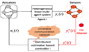
In this part, we describe the model of unknown and unbounded FDI attacks on the sensors of agents as shown in Fig. 1.

Definition 1

(FDI Sensor Attacks) This attack refers at time tsia0t^{a}_{si}\geq 0, an adversary injects any time-varying signals yia(t)py^{a}_{i}(t)\in\mathbb{R}^{p} into the measurement channel and thereby, modifying yi(t)y_{i}(t) into yic(t)py^{c}_{i}(t)\in\mathbb{R}^{p} adversely with a mapping gsg_{s}, i.e.,

gs:pp,yi(t)yic(t)=yi(t)+ϕiayia(t),i𝒱,g_{s}:\mathbb{R}^{p}\rightarrow\mathbb{R}^{p},\ y_{i}(t)\rightarrow y^{c}_{i}(t)=y_{i}(t)+\phi^{a}_{i}y^{a}_{i}(t),\ i\in\mathcal{V}, (6)

where yi(t)y_{i}(t) denotes the nominal output measurement in (1), yia(t)y^{a}_{i}(t) represents the disrupted signal that is injected into the sensors of agent ii and yic(t)y^{c}_{i}(t) denotes the corrupted measurements of agent ii. If agent ii is under attacks, ϕia=1\phi^{a}_{i}=1, otherwise, ϕia=0\phi^{a}_{i}=0.

Assumption 2

The FDI attack signals yia(t)y^{a}_{i}(t) are unknown and unbounded, while their time derivatives are assumed to be upper bounded but with certain unknown constants.

Remark 4

The adversary’s injections can be unbounded time-varying signals, which aim to manipulate or even destabilize the whole agent team’s behaviors. The slow-varying signals may not be easily detected. Hence, this assumption is more practical and reasonable in real-world applications.

II-E Main Objective

This work aims to achieve the resilient time-varying output formation tracking of linear multi-agent systems under FDI attacks and unreliable digraphs. We will develop a distributed estimator-based controller with corrupted individual output information and neighbor-based group output information. The control of agent ii is supposed to have the structure as depicted in Fig. 1. In the next section, we will specify the design procedure.

Problem 1

(Resilient Time-Varying Output Formation Tracking) Consider a leader-follower agent network consisting of (1)-(2). This multi-agent system is subject to malicious FDI attacks in (6) and communicates over unreliable digraphs 𝒢¯i,iΞ\bar{\mathcal{G}}_{i},i\in\Xi. Design a resilient distributed algorithm so that all agents achieve safe and reliable time-varying output formation tracking exponentially, i.e.,

limt(yi(t)yhi(t)y0(t))=0,i𝒱.\lim_{t\rightarrow\infty}(y_{i}(t)-y_{hi}(t)-y_{0}(t))=\textbf{0},\ i\in\mathcal{V}. (7)
Refer to caption
Figure 1: Modeling of malicious FDI attacks and unreliable communication.
Refer to caption
Figure 2: An illustration of a resilient distributed control framework for large-scale multi-agent networks under malicious FDI attacks and unreliable communication.
Remark 5

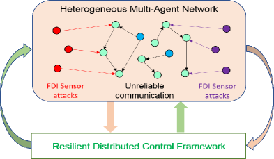
In contrast to many related existing works, solving Problem 1 is more challenging at least from the following aspects: 1) Adverse effects: as illustrated in Fig. 1, the unknown malicious FDI attackers can inject and manipulate the measured sensor data to destabilize the whole multi-agent network. Since the output of each agent is under FDI sensor attacks, only the uncompromised measurements will be available for a resilient distributed design; 2) Communication network: the unreliable communication makes topologies frequently switching rather than the fixed undirected or directed graphs in [5, 4, 7, 8, 6]. The underlying Laplacian matrices of each digraph are not necessarily positive definite; (3) Output time-varying formation tracking: many formation tracking algorithms in the existing works (e.g., [5, 4, 7, 8, 6]) require the full states of either the homogeneous or heterogeneous leader-follower system, which may not be available in practice. On the contrary, we adopt each agent’s corrupted outputs to develop a distributed observer-based controller; and (4) Design requirement: propose a novel resilient algorithm to deal with the adverse impacts of FDI attacks and unreliable communication. Due to the aforementioned aspects, the existing designs in [5, 4, 7, 8, 6] cannot be directly applied. A resilient distributed control framework is shown in Fig. 2.

III Exponential Distributed Stabilization for Resilient Time-Varying Output Formation Tracking

In this section, we will design a resilient distributed mechanism with an estimator-based control framework. To begin with, a distributed leader estimator is given to estimate and reconstruct the leader’s state for each follower over an unreliable communication network. Then, a resilient distributed output feedback controller is proposed to achieve time-varying output formation tracking. The procedure is given to design the estimator and controller gains.

III-A Reliable Distributed Leader Estimator Design

Denote an estimated state named as ζi\zeta_{i} to estimate the leader’s state x0(t)x_{0}(t). Then, a consensus tracking error is defined as

ξi(t)=i=1Naijσ(t)(ζi(t)ζj(t))+ai0σ(t)(ζi(t)x0(t)).\xi_{i}(t)=\sum\nolimits_{i=1}^{N}a^{\sigma(t)}_{ij}(\zeta_{i}(t)-\zeta_{j}(t))+a^{\sigma(t)}_{i0}(\zeta_{i}(t)-x_{0}(t)). (8)

In light of (8), a reliable distributed leader estimator using only output information is designed with a constant gain matrix K0K_{0},

ζ˙i(t)=A0ζi(t)K0C0ξi(t),i𝒱.\dot{\zeta}_{i}(t)=A_{0}\zeta_{i}(t)-K_{0}C_{0}\xi_{i}(t),\ i\in\mathcal{V}. (9)

Denote the tracking error ξ~i(t)=ζi(t)x0(t)\tilde{\xi}_{i}(t)=\zeta_{i}(t)-x_{0}(t) and its collective form is given by ξ~(t)=col(ξ~1(t),,ξ~N(t))\tilde{\xi}(t)=\text{col}(\tilde{\xi}_{1}(t),\cdots,\tilde{\xi}_{N}(t)). Then, combing (8) and (9) gives rise to the following closed-loop error system

ξ~˙(t)=[INA0(Hσ(t)K0C0)]ξ~(t).\dot{\tilde{\xi}}(t)=[I_{N}\otimes A_{0}-(H_{\sigma(t)}\otimes K_{0}C_{0})]\tilde{\xi}(t). (10)

Next, the following lemma is provided to establish a symmetric and positive definite matrix for directed graphs.

Lemma 2

Under Assumption 1, there exist positive definite diagonal matrices Θσ(t)=diag{θσ(t)1,,θσ(t)N}\Theta_{\sigma(t)}=\text{diag}\{\theta^{1}_{\sigma(t)},\cdots,\theta^{N}_{\sigma(t)}\} for each σ(t)Ξc\sigma(t)\in\Xi_{c}, so that Qσ(t)=Hσ(t)TΘσ(t)+Θσ(t)Hσ(t)>0Q_{\sigma(t)}=H_{\sigma(t)}^{T}\Theta_{\sigma(t)}+\Theta_{\sigma(t)}H_{\sigma(t)}>0.

Proof:

this result extends Lemma 1 from a fixed digraph to time-varying ones as shown in the existing works (e.g., [26]). The detailed proof is omitted due to space limitation. ∎

For notational convenience, denote

μ={maxiΞc{λmax(Θi)/λmin(Θi)},ifδ¯>1,1,ifδ¯=1,\mu=\left\{\begin{array}[]{c}\max_{i\in\Xi_{c}}\{\lambda_{max}(\Theta_{i})/\lambda_{min}(\Theta_{i})\},\ \text{if}\ \bar{\delta}>1,\\ 1,\ \ \ \ \ \ \ \ \ \ \ \ \ \ \ \ \ \ \ \ \ \ \ \ \ \ \ \ \ \ \ \ \ \ \ \ \ \ \text{if}\ \bar{\delta}=1,\end{array}\right. (11)

where Θi>0\Theta_{i}>0, iΞci\in\Xi_{c} are defined in Lemma 2, and further, let

λm\displaystyle\lambda_{m} =miniΞc{λmin(Θi1HiTΘi+Hi)}=miniΞc{λmin(Θi1Qi)},\displaystyle=\min_{i\in\Xi_{c}}\{\lambda_{min}(\Theta^{-1}_{i}H_{i}^{T}\Theta_{i}+H_{i})\}=\min_{i\in\Xi_{c}}\{\lambda_{min}(\Theta^{-1}_{i}Q_{i})\},
σm\displaystyle\sigma_{m} =maxiΞd{σmax(Φ1HiTΦ+Hi)},Φ=(i=1δ¯Θi)/δ¯,\displaystyle=\max_{i\in\Xi_{d}}\{\sigma_{max}(\Phi^{-1}H_{i}^{T}\Phi+H_{i})\},\ \Phi=(\sum_{i=1}^{\bar{\delta}}\Theta_{i})/\bar{\delta}, (12)

where Φ>0\Phi>0 denotes the average of Θi\Theta_{i}, iΞc\forall i\in\Xi_{c}, and moreover, it is not difficult to derive Φ<μΘi\Phi<\mu\Theta_{i}, iΞc\forall i\in\Xi_{c}.

Theorem 1

Suppose that Assumption 1 holds. If the distributed leader estimator is designed as (9) with K0=κ0P01C0TR01K_{0}=\kappa_{0}P^{-1}_{0}C^{T}_{0}R^{-1}_{0}, κ0(1/λm,ϵ/σm)\kappa_{0}\in(1/\lambda_{m},\epsilon/\sigma_{m}), then all the estimated states of the distributed estimator can globally exponentially converge to the leader’s state, provided that the scalars τa\tau_{a} and π\pi satisfy

τa>(lnμ)/(ηη)andπ<(αη)/(β+η),\displaystyle\tau_{a}>(\ln\mu)/(\eta^{*}-\eta)\ \text{and}\ \pi<(\alpha-\eta^{*})/(\beta+\eta^{*}), (13)

where μ1\mu\geq 1, α=λmin(Q0)/λmax(P0)\alpha=\lambda_{\min}(Q_{0})/\lambda_{\max}(P_{0}), η(0,α)\eta^{*}\in(0,\alpha), η(0,η)\eta\in(0,\eta^{*}), and β,P0>0\beta,P_{0}>0 are the solutions of an optimization problem:

minimizeβ>0,\text{minimize}\ \beta>0, (14)
s.t.{P0A0+A0TP0C0TR01C0+Q0<0,P0A0+A0TP0+ϵC0TR01C0βP0<0,s.t.\left\{\begin{array}[]{c}P_{0}A_{0}+A^{T}_{0}P_{0}-C^{T}_{0}R^{-1}_{0}C_{0}+Q_{0}<0,\\ P_{0}A_{0}+A^{T}_{0}P_{0}+\epsilon C^{T}_{0}R^{-1}_{0}C_{0}-\beta P_{0}<0,\end{array}\right. (15)

where R0R_{0} and Q0>IrQ_{0}>I_{r} are symmetric positive definite matrices.

Proof:

we construct the following piecewise Lyapunov functional candidate for the closed-loop error system in (10) as

V(t)={ξ~T(t)(Θσ(t)P0)ξ~(t),ifσ(t)Ξc,ξ~T(t)(ΦP0)ξ~(t),ifσ(t)Ξd.V(t)=\left\{\begin{array}[]{c}\tilde{\xi}^{T}(t)(\Theta_{\sigma(t)}\otimes P_{0})\tilde{\xi}(t),\ \text{if}\ \sigma(t)\in\Xi_{c},\\ \tilde{\xi}^{T}(t)(\Phi\otimes P_{0})\tilde{\xi}(t),\ \ \ \ \ \text{if}\ \sigma(t)\in\Xi_{d}.\end{array}\right. (16)

where Θσ(t)\Theta_{\sigma(t)} and Φ\Phi are defined in Lemma 2 and (12), respectively.

Next, the proof includes the following steps:

Step (i). we consider the case with σ(t)Ξc\sigma(t)\in\Xi_{c}. Taking the time derivative of (16) along (10) with K0=κ0P01C0TR01K_{0}=\kappa_{0}P^{-1}_{0}C^{T}_{0}R^{-1}_{0} yields

V˙(t)\displaystyle\dot{V}(t) =ξ~T(t)[Θσ(t)(P0A0+A0TP0)]ξ~(t)\displaystyle=\tilde{\xi}^{T}(t)[\Theta_{\sigma(t)}\otimes(P_{0}A_{0}+A^{T}_{0}P_{0})]\tilde{\xi}(t) (17)
κ0ξ~T(t)[(Hσ(t)TΘσ(t)+Θσ(t)Hσ(t))C0TR01C0)]ξ~(t).\displaystyle\ \ -\kappa_{0}\tilde{\xi}^{T}(t)[(H_{\sigma(t)}^{T}\Theta_{\sigma(t)}+\Theta_{\sigma(t)}H_{\sigma(t)})\otimes C^{T}_{0}R^{-1}_{0}C_{0})]\tilde{\xi}(t).

According to (15) and κ0>1/λm\kappa_{0}>1/\lambda_{m}, we have

V˙(t)\displaystyle\dot{V}(t) ξ~T(t)[Θσ(t)(P0A0+A0TP0C0TR01C0)]ξ~(t)\displaystyle\leq\tilde{\xi}^{T}(t)[\Theta_{\sigma(t)}\otimes(P_{0}A_{0}+A^{T}_{0}P_{0}-C^{T}_{0}R^{-1}_{0}C_{0})]\tilde{\xi}(t)
ξ~T(t)(Θσ(t)Q0)ξ~(t)αV(t),σ(t)Ξc,\displaystyle\leq-\tilde{\xi}^{T}(t)(\Theta_{\sigma(t)}\otimes Q_{0})\tilde{\xi}(t)\leq-\alpha V(t),\sigma(t)\in\Xi_{c}, (18)

where α=λmin(Q0)/λmax(P0)\alpha=\lambda_{\min}(Q_{0})/\lambda_{\max}(P_{0}) based on the fact that Q0λmin(Q0)Ir=αλmax(P0)IrαP0-Q_{0}\leq-\lambda_{\min}(Q_{0})I_{r}=-\alpha\lambda_{\max}(P_{0})I_{r}\leq-\alpha P_{0}.

Step (ii). consider the case with σ(t)Ξb\sigma(t)\in\Xi_{b}. Similarly, the time derivative of (16) along (10) with the fact that κ0σm<ϵ\kappa_{0}\sigma_{m}<\epsilon yields

V˙(t)\displaystyle\dot{V}(t) =ξ~T(t)[Φ(P0A0+A0TP0)]ξ~(t)κ0ξ~T(t)\displaystyle=\tilde{\xi}^{T}(t)[\Phi\otimes(P_{0}A_{0}+A^{T}_{0}P_{0})]\tilde{\xi}(t)-\kappa_{0}\tilde{\xi}^{T}(t)
×[(Hσ(t)TΦ+ΦHσ(t))C0TR01C0)]ξ~(t)\displaystyle\ \ \ \times[(H_{\sigma(t)}^{T}\Phi+\Phi H_{\sigma(t)})\otimes C^{T}_{0}R^{-1}_{0}C_{0})]\tilde{\xi}(t)
ξ~T(t)[Φ(P0A0+A0TP0)+κ0σmC0TR01C0)]ξ~(t)\displaystyle\leq\tilde{\xi}^{T}(t)[\Phi\otimes(P_{0}A_{0}+A^{T}_{0}P_{0})+\kappa_{0}\sigma_{m}C^{T}_{0}R^{-1}_{0}C_{0})]\tilde{\xi}(t)
ξ~T(t)(ΦβP0)ξ~(t)=βV(t),σ(t)Ξb.\displaystyle\leq\tilde{\xi}^{T}(t)(\Phi\otimes\beta P_{0})\tilde{\xi}(t)=\beta V(t),\sigma(t)\in\Xi_{b}. (19)

Step (iii). synthesizing Steps (i)-(ii) into one, it is obtained from (18) and (19) that for any t[tk,tk+1)t\in\left[t_{k},t_{k+1}\right), we can have

V(t){eα(ttk)V(tk),σ(t)Ξc,eβ(ttk)V(tk),σ(t)Ξb.V(t)\leq\left\{\begin{array}[]{c}e^{-\alpha(t-t_{k})}V(t_{k}),\ \sigma(t)\in\Xi_{c},\\ e^{\beta(t-t_{k})}V(t_{k}),\ \sigma(t)\in\Xi_{b}.\end{array}\right. (20)

Since σ(t)Ξ=ΞcΞb\sigma(t)\in\Xi=\Xi_{c}\cup\Xi_{b}, it further has for any t[tk,tk+1)t\in\left[t_{k},t_{k+1}\right),

V(t)eαTtkc(t)+βTtkb(t)V(tk).V(t)\leq e^{-\alpha T^{c}_{t_{k}}(t)+\beta T^{b}_{t_{k}}(t)}V(t_{k}). (21)

Suppose that there is no jump in the state ζi(t)\zeta_{i}(t) at the switching instant, i.e., ζi(tk)=ζi(tk)\zeta_{i}(t_{k})=\zeta_{i}(t_{k}^{-}). Further, using (16) gives rise to

V(t)μV(tk),μ1.V(t)\leq\mu V(t_{k}^{-}),\ \forall\mu\geq 1. (22)

Let Nσ(t)(t0,t)N_{\sigma(t)}(t_{0},t) denote the times of switching during [t0,t)[t_{0},t). Then, it follows from (21) and (22) that

V(t)\displaystyle V(t) μeβTtkb(t)αTtkc(t)V(tk)μeβTtk1b(t)αTtk1c(t)V(tk1)\displaystyle\leq\mu e^{\beta T^{b}_{t_{k}}(t)-\alpha T^{c}_{t_{k}}(t)}V(t_{k}^{-})\leq\mu e^{\beta T^{b}_{t_{k-1}}(t)-\alpha T^{c}_{t_{k-1}}(t)}V(t_{k-1})
μ2eαTtk1c(t)+βTtk1b(t)V(tk1)\displaystyle\leq\mu^{2}e^{-\alpha T^{c}_{t_{k-1}}(t)+\beta T^{b}_{t_{k-1}}(t)}V(t_{k-1}^{-})\ \leq\ \cdots
μNσ(t)(t0,t)eαTt0c(t)+βTt0b(t)V(t0)\displaystyle\leq\mu^{N_{\sigma(t)}(t_{0},t)}e^{-\alpha T^{c}_{t_{0}}(t)+\beta T^{b}_{t_{0}}(t)}V(t_{0})
=eNσ(t)(t0,t)ln(μ)αTt0c(t)+βTt0b(t)V(t0).\displaystyle=e^{N_{\sigma(t)}(t_{0},t)\ln(\mu)-\alpha T^{c}_{t_{0}}(t)+\beta T^{b}_{t_{0}}(t)}V(t_{0}). (23)

On one hand, based on Assumption 1, we get Tt0b(t)πTt0c(t)T^{b}_{t_{0}}(t)\leq\pi T^{c}_{t_{0}}(t). On the other hand, π<(αη)/(β+η)\pi<(\alpha-\eta^{*})/(\beta+\eta^{*}) in (13). Thus, we get

βTt0b(t)αTt0c(t)η(Tt0c(t)+Tt0b(t))=η(tt0).\beta T^{b}_{t_{0}}(t)-\alpha T^{c}_{t_{0}}(t)\leq-\eta^{\ast}(T^{c}_{t_{0}}(t)+T^{b}_{t_{0}}(t))=-\eta^{\ast}(t-t_{0}). (24)

In addition, according to the average dwell time definition in the existing works, e.g., [12], Nσ(t)(t0,t)N0+(tt0)/τaN_{\sigma(t)}(t_{0},t)\leq N_{0}+(t-t_{0})/\tau_{a} for all tt0t\geq t_{0}. Since τa>(ln(μ))/(ηη)\tau_{a}>(\ln(\mu))/(\eta^{*}-\eta) in (13), we have

eNσ(t)(t0,t)ln(μ)e(N0+tt0τa)ln(μ)eN0ln(μ)e(ηη)(tt0).e^{N_{\sigma(t)}(t_{0},t)\ln(\mu)}\leq e^{(N_{0}+\frac{t-t_{0}}{\tau_{a}})\ln(\mu)}\leq e^{N_{0}\ln(\mu)}e^{(\eta^{*}-\eta)(t-t_{0})}. (25)

Combining (23)-(25) yields: V(t)eN0ln(μ)eη(tt0)V(t0)V(t)\leq e^{N_{0}\ln(\mu)}e^{-\eta(t-t_{0})}V(t_{0}). Hence, it follows from (16) that we have

ξ~i(t)φeη2(tt0)ξ~i(t0),\hskip 10.00002pt\|\tilde{\xi}_{i}(t)\|\leq\varphi e^{-\frac{\eta}{2}(t-t_{0})}\|\tilde{\xi}_{i}(t_{0})\|, (26)

where φ=(aeN0ln(μ)/b)12\varphi=(ae^{N_{0}\ln(\mu)}/b)^{\frac{1}{2}}, a=maxiΞc{λmax(θijP0),λmax(ΦP0)}a=\max_{i\in\Xi_{c}}\{\lambda_{\max}(\theta^{j}_{i}P_{0}),\lambda_{\max}(\Phi\\ P_{0})\} and b=miniΞc{λmin(θijP0),λmin(ΦP0)}b=\min_{i\in\Xi_{c}}\{\lambda_{\min}(\theta^{j}_{i}P_{0}),\lambda_{\min}(\Phi P_{0})\}, j𝒱j\in\mathcal{V}. ∎

III-B Resilient Distributed Control against FDI Sensor Attacks

In this subsection, we propose a novel resilient mechanism to achieve exponential output formation tracking in the presence of FDI sensor attacks in (6). Under sensor attacks, the output yi(t)y_{i}(t) is corrupted and only the corrupted yic(t)=yi(t)+ϕiayia(t)y^{c}_{i}(t)=y_{i}(t)+\phi^{a}_{i}y^{a}_{i}(t) can be measured. To deal with these FDI sensor attacks, a novel resilient distributed output feedback controller is developed as

ui(t)\displaystyle u_{i}(t) =K1ix^i(t)+K2iζi(t)+K3ihi(t),\displaystyle=K_{1i}\hat{x}_{i}(t)+K_{2i}\zeta_{i}(t)+K_{3i}h_{i}(t), (27)
x^˙i(t)\displaystyle\dot{\hat{x}}_{i}(t) =Aix^i(t)+Biui(t)+Liy~i(t),\displaystyle=A_{i}\hat{x}_{i}(t)+B_{i}u_{i}(t)+L_{i}\tilde{y}_{i}(t), (28)

where K1i,K2i,K3i,LiK_{1i},K_{2i},K_{3i},L_{i} are controller and observer gain matrices to be determined later, x^i(t)\hat{x}_{i}(t) represents the observed state of the observer, ζi(t)\zeta_{i}(t) is the estimate of the leader’s state designed in (8) and (9), hi(t)h_{i}(t) is the time-varying formation vector defined in (4), and y~i(t)\tilde{y}_{i}(t) denotes the measurable error term described by

y~i(t)=yic(t)y^i(t)y^ia(t),i𝒱,\tilde{y}_{i}(t)=y^{c}_{i}(t)-\hat{y}_{i}(t)-\hat{y}^{a}_{i}(t),\ i\in\mathcal{V}, (29)

where y^i(t)=Cix^i(t)\hat{y}_{i}(t)=C_{i}\hat{x}_{i}(t) is an estimation of the uncorrupted output measurement yi(t)y_{i}(t), and y^ia(t)\hat{y}^{a}_{i}(t) is an estimation of unknown sensor attacks ϕiayia(t)\phi^{a}_{i}y^{a}_{i}(t), which is updated through the following design:

y^˙ia(t)=Mi(yic(t)y^i(t)y^ia(t))+fia(t),\dot{\hat{y}}^{a}_{i}(t)=M_{i}(y^{c}_{i}(t)-\hat{y}_{i}(t)-\hat{y}^{a}_{i}(t))+f^{a}_{i}(t), (30)

where MiM_{i} is a gain matrix with appropriate dimensions and fia(t)f^{a}_{i}(t) denotes a compensation signal to be determined later.

Next, we denote two estimated errors:

x~i(t)=xi(t)x^i(t),y~ia(t)=ϕiayia(t)y^ia(t).\tilde{x}_{i}(t)=x_{i}(t)-\hat{x}_{i}(t),\ \tilde{y}^{a}_{i}(t)=\phi^{a}_{i}y^{a}_{i}(t)-\hat{y}^{a}_{i}(t). (31)

Then, based on (28)-(30), we can obtain that

x~˙i(t)\displaystyle\dot{\tilde{x}}_{i}(t) =(AiLiCi)x~i(t)Liy~ia(t),\displaystyle=(A_{i}-L_{i}C_{i})\tilde{x}_{i}(t)-L_{i}\tilde{y}^{a}_{i}(t), (32)
y~˙ia(t)\displaystyle\dot{\tilde{y}}^{a}_{i}(t) =Miy~ia(t)MiCix~i(t)+ϕiay˙ia(t)fia(t).\displaystyle=-M_{i}\tilde{y}^{a}_{i}(t)-M_{i}C_{i}\tilde{x}_{i}(t)+\phi^{a}_{i}\dot{y}^{a}_{i}(t)-f^{a}_{i}(t). (33)

To achieve the main objective of this paper, we need to analyze the global exponential convergence of x~i(t)\tilde{x}_{i}(t) and y~ia(t)\tilde{y}^{a}_{i}(t). Denote ϱi=col(x~i(t),y~ia(t))ni+p\varrho_{i}=\text{col}(\tilde{x}_{i}(t),\tilde{y}^{a}_{i}(t))\in\mathbb{R}^{n_{i}+p} as an augmented error variable. Further, it follows from (32)-(33) that we can derive the following closed-loop error system described by

ϱ˙i(t)=Aϱiϱi(t)+Bϱi[ϕiay˙ia(t)fia(t)],\dot{\varrho}_{i}(t)=A_{\varrho i}\varrho_{i}(t)+B_{\varrho i}\left[\phi^{a}_{i}\dot{y}^{a}_{i}(t)-f^{a}_{i}(t)\right], (34)
Aϱi=[AiLiCiLiMiCiMi],Bϱi=[0ni×pIp].A_{\varrho i}=\left[\begin{array}[]{cc}A_{i}-L_{i}C_{i}&-L_{i}\\ -M_{i}C_{i}&-M_{i}\end{array}\right],\ B_{\varrho i}=\left[\begin{array}[]{c}\textbf{0}_{n_{i}\times p}\\ I_{p}\end{array}\right]. (35)

Before presenting the convergence of ϱi\varrho_{i}, the following assumption is made to facilitate stability analysis.

Assumption 3

The pair (Ai,CiAi)(A_{i},C_{i}A_{i}) is observable.

Proposition 1

Under Assumption 3, there exists appropriate observer gain matrices LiL_{i} and MiM_{i} so that AϱiA_{\varrho i} in (35) is Hurwitz, i.e., there exists a matrix Pϱi>0P_{\varrho i}>0 such that

PϱiAϱi+AϱiTPϱi=Qϱifor anyQϱi>0.P_{\varrho i}A_{\varrho i}+A^{T}_{\varrho i}P_{\varrho i}=-Q_{\varrho i}\ \text{for any}\ Q_{\varrho i}>0. (36)
Proof:

according to (35), we can obtain that

[AiLiCiLiMiCiMi]Aϱi=[Ai0ni×p0p×ni0p×p]A¯i+[LiMi][CiIp]C¯i.\underbrace{\left[\begin{array}[]{cc}A_{i}-L_{i}C_{i}&-L_{i}\\ -M_{i}C_{i}&-M_{i}\end{array}\right]}_{A_{\varrho i}}=\underbrace{\left[\begin{array}[]{cc}A_{i}&\textbf{0}_{n_{i}\times p}\\ \textbf{0}_{p\times n_{i}}&\textbf{0}_{p\times p}\end{array}\right]}_{\bar{A}_{i}}+\left[\begin{array}[]{c}-L_{i}\\ M_{i}\end{array}\right]\underbrace{\left[\begin{array}[]{l}C_{i}\ I_{p}\end{array}\right]}_{\bar{C}_{i}}.

Then, it is observed that the matrix pair (A¯i,C¯i)(\bar{A}_{i},\bar{C}_{i}) is observable if and only if rank[(C¯i)T(C¯iA¯i)T(C¯iA¯ini+p1)T]T=ni+p\text{rank}\left[(\bar{C}_{i})^{T}\ (\bar{C}_{i}\bar{A}_{i})^{T}\ \cdots\ (\bar{C}_{i}\bar{A}_{i}^{n_{i}+p-1})^{T}\right]^{T}=n_{i}+p, which is equivalent to the following expression

rank[CiAiCiAi2CiAini+p1]=nirank[CiAiCiAi2CiAini]=ni,\text{rank}\left[\begin{array}[]{cc}C_{i}A_{i}\\ C_{i}A^{2}_{i}\\ \vdots\\ C_{i}A^{n_{i}+p-1}_{i}\end{array}\right]=n_{i}\Longleftrightarrow\text{rank}\left[\begin{array}[]{cc}C_{i}A_{i}\\ C_{i}A^{2}_{i}\\ \vdots\\ C_{i}A^{n_{i}}_{i}\end{array}\right]=n_{i}, (37)

where the second equation is guaranteed according to the Cayley-Hamilton theorem with Aini×niA_{i}\in\mathbb{R}^{n_{i}\times n_{i}} and p1p\geq 1.

Based on Assumption 3, we have

rank[[CiCiAiCiAini1]Ai]=rank[CiAiCiAiAiCiAini1Ai]=ni.\text{rank}\left[\left[\begin{array}[]{cc}C_{i}\\ C_{i}A_{i}\\ \vdots\\ C_{i}A^{n_{i}-1}_{i}\end{array}\right]A_{i}\right]=\text{rank}\left[\begin{array}[]{cc}C_{i}A_{i}\\ C_{i}A_{i}A_{i}\\ \vdots\\ C_{i}A^{n_{i}-1}_{i}A_{i}\end{array}\right]=n_{i}. (38)

Thus, LiL_{i} and MiM_{i} can be chosen such that AϱiA_{\varrho i} is Hurwitz. That is, (36) is obtained, and the proof is completed. ∎

Next, we present the global exponential convergence of ϱi=col(x~i(t),y~ia(t))\varrho_{i}=\text{col}(\tilde{x}_{i}(t),\tilde{y}^{a}_{i}(t)) in the closed-loop error system (34).

Proposition 2

Suppose that Assumptions 1-3 hold. For leader -follower multi-agent systems in (1)-(4) subject to sensor attacks in (6), the global exponential convergence of x~i(t)\tilde{x}_{i}(t) and y~ia(t)\tilde{y}^{a}_{i}(t) can be guaranteed under the proposed resilient distributed controller in (27)-(30), provided that fia(t)f^{a}_{i}(t) is designed as

fia(t)\displaystyle f^{a}_{i}(t) =diag{ϱ¯ϑij}ε^i(t),ϱ¯ϑij=ϱ¯ij/ϱ¯ij2+ϑij2(t),\displaystyle=\text{diag}\left\{\bar{\varrho}_{\vartheta ij}\right\}\hat{\varepsilon}_{i}(t),\ \bar{\varrho}_{\vartheta ij}=\bar{\varrho}_{ij}/\sqrt{\bar{\varrho}^{2}_{ij}+\vartheta^{2}_{ij}(t)},
ε^˙i(t)\displaystyle\dot{\hat{\varepsilon}}_{i}(t) =diag{ϱ¯ϑij}ϱ¯i,ϱ¯i=BϱiTC¯iTC¯iPiC¯iTC¯iϱi,\displaystyle=\text{diag}\{\bar{\varrho}_{\vartheta ij}\}\bar{\varrho}_{i},\ \bar{\varrho}_{i}=B^{T}_{\varrho i}\bar{C}^{T}_{i}\bar{C}_{i}P_{i}\bar{C}^{T}_{i}\bar{C}_{i}\varrho_{i}, (39)

where Pi>0P_{i}>0 is to be determined later, ε^i\hat{\varepsilon}_{i} denotes the estimate of εi=supt0|ϕiay˙ia(t)|\varepsilon_{i}=\text{sup}_{t\geq 0}|\phi^{a}_{i}\dot{y}^{a}_{i}(t)|, ϱ¯ij\bar{\varrho}_{ij} is the jjth element of ϱ¯i\bar{\varrho}_{i}, and ϑij(t)>0\vartheta_{ij}(t)>0 is an integrable function such that 0tϑij(s)𝑑sϑ\int_{0}^{t}\vartheta_{ij}(s)ds\leq\vartheta^{*} for certain scalar ϑ>0\vartheta^{*}>0, i.e., ϑij(t)=exp(ϑ0ijt)\vartheta_{ij}(t)=\text{exp}(-\vartheta_{0ij}t) with a scalar ϑ0ij>0\vartheta_{0ij}>0.

Proof:

it follows from (29) and (31) that

y~i(t)=yic(t)y^ia(t)y^i(t)=Cix~i+y~ia(t)=C¯iϱi.\tilde{y}_{i}(t)=y^{c}_{i}(t)-\hat{y}^{a}_{i}(t)-\hat{y}_{i}(t)=C_{i}\tilde{x}_{i}+\tilde{y}^{a}_{i}(t)=\bar{C}_{i}\varrho_{i}.

Substituting (39) into (34) gives rise to

ϱ˙i(t)=Aϱiϱi(t)+Bϱi[ϕiay˙ia(t)diag{ϱ¯ijϱ¯ij2+ϑij2(t)}ε^i(t)].\dot{\varrho}_{i}(t)=A_{\varrho i}\varrho_{i}(t)+B_{\varrho i}[\phi^{a}_{i}\dot{y}^{a}_{i}(t)-\text{diag}\left\{\frac{\bar{\varrho}_{ij}}{\sqrt{\bar{\varrho}^{2}_{ij}+\vartheta^{2}_{ij}(t)}}\right\}\hat{\varepsilon}_{i}(t)].

Consider the following Lyapunov functional candidate

Wi(t)=(C¯iTC¯iϱi)TPi(C¯iTC¯iϱi)+ε~iT(t)ε~i(t),W_{i}(t)=\left(\bar{C}^{T}_{i}\bar{C}_{i}\varrho_{i}\right)^{T}P_{i}\left(\bar{C}^{T}_{i}\bar{C}_{i}\varrho_{i}\right)+\tilde{\varepsilon}^{T}_{i}(t)\tilde{\varepsilon}_{i}(t), (40)

where Pi>0P_{i}>0 can be selected such that AϱiPϱi+PϱiAϱiT=QϱiA_{\varrho i}P_{\varrho i}+P_{\varrho i}A^{T}_{\varrho i}=-Q_{\varrho i} in (36) holds with Pϱi=C¯iTC¯iPiC¯iTC¯iP_{\varrho i}=\bar{C}^{T}_{i}\bar{C}_{i}P_{i}\bar{C}^{T}_{i}\bar{C}_{i}, C¯i=[Ci,Ip]\bar{C}_{i}=[C_{i},I_{p}], and ε~i=εiε^i\tilde{\varepsilon}_{i}=\varepsilon_{i}-\hat{\varepsilon}_{i} denotes the estimated error.

Then, the time derivative of Wi(t)W_{i}(t) along the trajectories of the closed-loop error system (34) is described by

W˙i(t)\displaystyle\dot{W}_{i}(t) =2ϱiT(t)PϱiAϱiϱi(t)+2ϱiT(t)PϱiBϱi[ϕiay˙ia(t)\displaystyle=2\varrho^{T}_{i}(t)P_{\varrho i}A_{\varrho i}\varrho_{i}(t)+2\varrho^{T}_{i}(t)P_{\varrho i}B_{\varrho i}[\phi^{a}_{i}\dot{y}^{a}_{i}(t)
diag{ϱ¯ijϱ¯ij2+ϑij2(t)}ε^i(t)]2ε~Ti(t)ε^˙i(t)\displaystyle\ \ \ -\text{diag}\left\{\frac{\bar{\varrho}_{ij}}{\sqrt{\bar{\varrho}^{2}_{ij}+\vartheta^{2}_{ij}(t)}}\right\}\hat{\varepsilon}_{i}(t)]-2\tilde{\varepsilon}^{T}_{i}(t)\dot{\hat{\varepsilon}}_{i}(t)
=ϱiT(t)(AϱiPϱi+PϱiAϱiT)ϱi(t)+2ϱiT(t)PϱiBϱi\displaystyle=\varrho^{T}_{i}(t)(A_{\varrho i}P_{\varrho i}+P_{\varrho i}A^{T}_{\varrho i})\varrho_{i}(t)+2\varrho^{T}_{i}(t)P_{\varrho i}B_{\varrho i}
×[ϕiay˙ia(t)diag{ϱ¯ijϱ¯ij2+ϑij2(t)}ε^i(t)]\displaystyle\ \ \ \times[\phi^{a}_{i}\dot{y}^{a}_{i}(t)-\text{diag}\left\{\frac{\bar{\varrho}_{ij}}{\sqrt{\bar{\varrho}^{2}_{ij}+\vartheta^{2}_{ij}(t)}}\right\}\hat{\varepsilon}_{i}(t)]
(εiε^i)Tdiag{2ϱ¯ijϱ¯ij2+ϑij2(t)}BϱiTPϱiϱi(t).\displaystyle\ \ -(\varepsilon_{i}-\hat{\varepsilon}_{i})^{T}\text{diag}\left\{\frac{2\bar{\varrho}_{ij}}{\sqrt{\bar{\varrho}^{2}_{ij}+\vartheta^{2}_{ij}(t)}}\right\}B^{T}_{\varrho i}P_{\varrho i}\varrho_{i}(t). (41)

Let εij\varepsilon_{ij} represent the jjth element of the vector εi\varepsilon_{i}. Since |ϱ¯ij|ϱ¯ijϱ¯ij/ϱ¯ij2+ϑij2(t)ϑij(t)|\bar{\varrho}_{ij}|-\bar{\varrho}_{ij}\bar{\varrho}_{ij}/\sqrt{\bar{\varrho}^{2}_{ij}+\vartheta^{2}_{ij}(t)}\leq\vartheta_{ij}(t), we have

W˙i(t)\displaystyle\dot{W}_{i}(t) =ϱiTQϱiϱi+2ϱ¯iT[ϕiay˙ia(t)diag{ϱ¯ijϱ¯ij2+ϑij2(t)}εi]\displaystyle=-\varrho^{T}_{i}Q_{\varrho i}\varrho_{i}+2\bar{\varrho}^{T}_{i}[\phi^{a}_{i}\dot{y}^{a}_{i}(t)-\text{diag}\{\frac{\bar{\varrho}_{ij}}{\sqrt{\bar{\varrho}^{2}_{ij}+\vartheta^{2}_{ij}(t)}}\}\varepsilon_{i}]
ϱiTQϱiϱi+j=1n[|ϱ¯ij|εijϱ¯ij2εij/ϱ¯ij2+ϑij2(t)]\displaystyle\leq-\varrho^{T}_{i}Q_{\varrho i}\varrho_{i}+\sum^{n}_{j=1}[|\bar{\varrho}_{ij}|\varepsilon_{ij}-\bar{\varrho}^{2}_{ij}\varepsilon_{ij}/\sqrt{\bar{\varrho}^{2}_{ij}+\vartheta^{2}_{ij}(t)}]
λmin(Qϱi)ϱiTϱi+j=1nϑij(t)εij.\displaystyle\leq-\lambda_{min}(Q_{\varrho i})\varrho^{T}_{i}\varrho_{i}+\sum^{n}_{j=1}\vartheta_{ij}(t)\varepsilon_{ij}. (42)

Integrating both the sides of (42) gives rise to Wi(t)Wi(0)0tλmin(Qϱi)ϱiTϱi𝑑s+IϑW_{i}(t)\leq W_{i}(0)-\int_{0}^{t}\lambda_{min}(Q_{\varrho i})\varrho^{T}_{i}\varrho_{i}ds+I_{\vartheta}, where Iϑ=0tj=1nϑij(s)εijdsI_{\vartheta}=\int_{0}^{t}\sum^{n}_{j=1}\vartheta_{ij}(s)\varepsilon_{ij}ds. By Assumption 2, we obtain that εijεmax=maxi𝒱{ϕiay˙ia(t)}\varepsilon_{ij}\leq\varepsilon_{max}=\max_{i\in\mathcal{V}}\{\|\phi^{a}_{i}\dot{y}^{a}_{i}(t)\|\} holds. In addition, recalling the property of the integrable function ϑij(t)\vartheta_{ij}(t) with 0tϑij(s)𝑑sϑ\int_{0}^{t}\vartheta_{ij}(s)ds\leq\vartheta^{*} for ϑ>0\vartheta^{*}>0, we have |Iϑ|c0|I_{\vartheta}|\leq c_{0} for certain scalar c0>0c_{0}>0. Thus, the above inequality implies that all signals in Wi(t)W_{i}(t) are bounded. Denote di0=Wi(0)+c0d_{i0}=W_{i}(0)+c_{0},

λmin(Pϱi)ϱiTϱiWi(t)0tλmin(Qϱi)ϱiTϱi𝑑s+di0.\lambda_{min}(P_{\varrho i})\varrho^{T}_{i}\varrho_{i}\leq W_{i}(t)\leq-\int_{0}^{t}\lambda_{min}(Q_{\varrho i})\varrho^{T}_{i}\varrho_{i}ds+d_{i0}. (43)

Recalling the Bellman-Gronwall Lemma in [27], (43) is further described by ϱi2di0λmin(Pϱi)exp(λmin(Qϱi)λmin(Pϱi)t)\|\varrho_{i}\|^{2}\leq\sqrt{\frac{d_{i0}}{\lambda_{min}(P_{\varrho i})}}\text{exp}\left(-\frac{\lambda_{min}(Q_{\varrho i})}{\lambda_{min}(P_{\varrho i})}t\right). Hence, it is concluded that both x~i(t)\tilde{x}_{i}(t) and y~ia(t)\tilde{y}^{a}_{i}(t) can globally exponentially converge towards zero, and the proof is finished. ∎

Next, we are ready to present the resilient time-varying output formation tracking result, which is summarized below.

Theorem 2

Consider the heterogeneous leader-follower multi -agent system (1)-(4) subject to FDI sensor attacks and unreliable digraphs. Suppose that Assumptions 1-3 hold. Under the proposed resilient algorithm in (27)-(30), the time-varying output formation tracking can be achieved exponentially, provided that the observer gain matrices LiL_{i}, MiM_{i} are selected such that AϱiA_{\varrho i} in (35) is Hurwitz, the controller gain matrix K1iK_{1i} is chosen such that Ai+BiK1iA_{i}+B_{i}K_{1i} is Hurwitz, and K2i,K3iK_{2i},K_{3i} are designed as

K2i=UiK1iXi,K3i=UhiK1iXhi,K_{2i}=U_{i}-K_{1i}X_{i},\ K_{3i}=U_{hi}-K_{1i}X_{hi}, (44)

where (Xi,Ui)(X_{i},U_{i}) and (Xhi,Uhi)(X_{hi},U_{hi}) are the solution of the well-known regulated equations in (3) and (5), respectively.

Proof:

define a formation transformation coordinate as

x¯i(t)=xi(t)Xix0(t)Xhihi(t).\bar{x}_{i}(t)=x_{i}(t)-X_{i}x_{0}(t)-X_{hi}h_{i}(t). (45)

Then, the time derivative of x¯i(t)\bar{x}_{i}(t) is described as

x¯˙i(t)\displaystyle\dot{\bar{x}}_{i}(t) =Aixi(t)+Biui(t)XiA0x0(t)XhiAhihi(t)\displaystyle=A_{i}x_{i}(t)+B_{i}u_{i}(t)-X_{i}A_{0}x_{0}(t)-X_{hi}A_{hi}h_{i}(t)
=Aixi(t)+Bi(K1ix^i(t)+K2iζi(t)+K3ihi(t))\displaystyle=A_{i}x_{i}(t)+B_{i}(K_{1i}\hat{x}_{i}(t)+K_{2i}\zeta_{i}(t)+K_{3i}h_{i}(t))
XiA0x0(t)XhiAhihi(t)\displaystyle\ \ \ -X_{i}A_{0}x_{0}(t)-X_{hi}A_{hi}h_{i}(t)
=(Ai+BiK1i)xi(t)BiK1ix~i(t)+BiK2iζi(t)\displaystyle=(A_{i}+B_{i}K_{1i})x_{i}(t)-B_{i}K_{1i}\tilde{x}_{i}(t)+B_{i}K_{2i}\zeta_{i}(t)
+BiK3ihi(t)XiA0x0(t)XhiAhihi(t).\displaystyle\ \ \ +B_{i}K_{3i}h_{i}(t)-X_{i}A_{0}x_{0}(t)-X_{hi}A_{hi}h_{i}(t). (46)

Substituting (3) and (5) into (46) further gives rise to

x¯˙i(t)\displaystyle\dot{\bar{x}}_{i}(t) =(Ai+BiK1i)(x¯i(t)+Xix0(t)+Xhihi(t))\displaystyle=(A_{i}+B_{i}K_{1i})(\bar{x}_{i}(t)+X_{i}x_{0}(t)+X_{hi}h_{i}(t))
BiK1ix~i(t)+BiK2iζi(t)+BiK3ihi(t)\displaystyle\ \ \ -B_{i}K_{1i}\tilde{x}_{i}(t)+B_{i}K_{2i}\zeta_{i}(t)+B_{i}K_{3i}h_{i}(t)
(AiXi+BiUi)x0(t)(AiXhi+BiUhi)hi(t)\displaystyle\ \ \ -(A_{i}X_{i}+B_{i}U_{i})x_{0}(t)-(A_{i}X_{hi}+B_{i}U_{hi})h_{i}(t)
=(Ai+BiK1i)x¯i(t)+BiK1iXix0(t)+BiK1iXhihi(t)\displaystyle=(A_{i}+B_{i}K_{1i})\bar{x}_{i}(t)+B_{i}K_{1i}X_{i}x_{0}(t)+B_{i}K_{1i}X_{hi}h_{i}(t)
BiK1ix~i(t)+BiK2iζi(t)+BiK3ihi(t)\displaystyle\ \ \ -B_{i}K_{1i}\tilde{x}_{i}(t)+B_{i}K_{2i}\zeta_{i}(t)+B_{i}K_{3i}h_{i}(t)
BiUix0(t)BiUhihi(t).\displaystyle\ \ \ -B_{i}U_{i}x_{0}(t)-B_{i}U_{hi}h_{i}(t). (47)

Choose K2i=UiK1iXiK_{2i}=U_{i}-K_{1i}X_{i} and K3i=UhiK1iXhiK_{3i}=U_{hi}-K_{1i}X_{hi} in (44). The equation in (47) is further rewritten as

x¯˙i(t)\displaystyle\dot{\bar{x}}_{i}(t) =(Ai+BiK1i)x¯i(t)+BiK1iXix0(t)+BiK1iXhihi(t)\displaystyle=(A_{i}+B_{i}K_{1i})\bar{x}_{i}(t)+B_{i}K_{1i}X_{i}x_{0}(t)+B_{i}K_{1i}X_{hi}h_{i}(t)
BiK1ix~i(t)+Bi(UiK1iXi)ζi(t)BiUix0(t)\displaystyle\ \ \ -B_{i}K_{1i}\tilde{x}_{i}(t)+B_{i}(U_{i}-K_{1i}X_{i})\zeta_{i}(t)-B_{i}U_{i}x_{0}(t)
+Bi(UhiK1iXhi)hi(t)BiUhihi(t)\displaystyle\ \ \ +B_{i}(U_{hi}-K_{1i}X_{hi})h_{i}(t)-B_{i}U_{hi}h_{i}(t)
=(Ai+BiK1i)x¯i(t)BiK1ix~i(t)+BiK2iξ~i(t).\displaystyle=(A_{i}+B_{i}K_{1i})\bar{x}_{i}(t)-B_{i}K_{1i}\tilde{x}_{i}(t)+B_{i}K_{2i}\tilde{\xi}_{i}(t). (48)

It follows from Theorem 1 that ξ~i(t)\tilde{\xi}_{i}(t) exponentially converges to zero and from Proposition 2 that x~i(t)\tilde{x}_{i}(t) exponentially converges to zero. Moreover, K1iK_{1i} is selected so that Ai+BiK1iA_{i}+B_{i}K_{1i} is Hurwitz. Thus, it is concluded from (48) that x¯i(t)\bar{x}_{i}(t) can converge to zero exponentially, i.e., limtx¯i(t)=0\lim_{t\rightarrow\infty}\bar{x}_{i}(t)=\textbf{0} exponentially.

Denote the time-varying output formation tracking error as

ei(t)\displaystyle e_{i}(t) =yi(t)yhi(t)y0(t)=Cixi(t)Chihi(t)C0x0(t)\displaystyle=y_{i}(t)-y_{hi}(t)-y_{0}(t)=C_{i}x_{i}(t)-C_{hi}h_{i}(t)-C_{0}x_{0}(t)
=Ci[x¯i(t)+Xix0(t)+Xhihi(t)]Chihi(t)C0x0(t)\displaystyle=C_{i}[\bar{x}_{i}(t)+X_{i}x_{0}(t)+X_{hi}h_{i}(t)]-C_{hi}h_{i}(t)-C_{0}x_{0}(t)
=Cix¯i(t)+(CiXiC0)x0(t)+(CiXhiChi)hi(t).\displaystyle=C_{i}\bar{x}_{i}(t)+(C_{i}X_{i}-C_{0})x_{0}(t)+(C_{i}X_{hi}-C_{hi})h_{i}(t). (49)

Due to the fact that CiXi=C0C_{i}X_{i}=C_{0} and CiXhi=ChiC_{i}X_{hi}=C_{hi}, then we can have ei(t)=Cix¯i(t)e_{i}(t)=C_{i}\bar{x}_{i}(t). Since limtx¯i(t)=0\lim_{t\rightarrow\infty}\bar{x}_{i}(t)=\textbf{0} exponentially, it is concluded that limtei(t)=0\lim_{t\rightarrow\infty}e_{i}(t)=\textbf{0} exponentially. Hence, the global exponential time-varying output formation tracking is achieved for the heterogeneous linear multi-agent systems in the presence of FDI sensor attacks and unreliable digraphs. ∎

IV Resilient Time-Varying Formation-Containment Tracking with Multiple Leaders

Consider a linear multi-agent network consisted of NN followers and MM leaders with their dynamics described by

{x˙i(t)=Aixi(t)+Biui(t),yi(t)=Cixi(t),i𝔽,x˙k(t)=A0xk(t),yk(t)=C0xk(t),k𝕃,\left\{\begin{array}[]{c}\dot{x}_{i}(t)=A_{i}x_{i}(t)+B_{i}u_{i}(t),\ y_{i}(t)=C_{i}x_{i}(t),\ i\in\mathbb{F},\\ \dot{x}_{k}(t)=A_{0}x_{k}(t),\ y_{k}(t)=C_{0}x_{k}(t),\ k\in\mathbb{L},\end{array}\right. (50)

where 𝔽={1,2,,N}\mathbb{F}=\{1,2,\cdots,N\} and 𝕃={N+1,N+2,,N+M}\mathbb{L}=\{N+1,N+2,\cdots,N+M\} are the sets of the followers and leaders, respectively, and xkx_{k} and yky_{k} are the state and output of the kkth leader, respectively.

In the networked agent team, the leaders do not have incoming edges and the followers have the relative neighboring information. The well-informed and unwell-informed followers are defined.

Definition 2

[5] A follower is called the well-informed one if it has incoming edges from all leaders, and the uniformed follower if it has no incoming edges from any leaders.

Definition 3

[28] A set 𝒞n\mathcal{C}\subseteq\mathbb{R}^{n} can be said to be convex if (1λ)x+λy𝒞(1-\lambda)x+\lambda y\in\mathcal{C} holds for any x,y𝒞x,y\in\mathcal{C} and λ[0,1]\lambda\in[0,1]. Then, the convex hull of a finite set of points Z={z1,z2,,zn}Z=\{z_{1},z_{2},\cdots,z_{n}\} is the minimal convex set containing all points in ZZ, i.e., Co(Z)={k=1nγkzk|zkZ,γk,γk0,k=1nγk=1}\text{Co}(Z)=\{\sum^{n}_{k=1}\gamma_{k}z_{k}|z_{k}\in Z,\gamma_{k}\in\mathbb{R},\gamma_{k}\geq 0,\sum^{n}_{k=1}\gamma_{k}=1\}. That is, k=1nγkzk\sum^{n}_{k=1}\gamma_{k}z_{k} is the convex combination of zkz_{k}.

Problem 2

The multi-agent system (50) subject to unreliable digraphs and unknown and unbounded sensor attacks in (6) is said to achieve resilient time-varying formation-containment tracking if there exist a scalar γk>0\gamma_{k}>0, k𝕃k\in\mathbb{L} that satisfies k=N+1N+Mγk=1\sum_{k=N+1}^{N+M}\gamma_{k}=1 such that for any initial states, the closed-loop system is globally stable and the output formation-containment tracking satisfies

limt(yi(t)yhi(t)k=N+1N+Mγkyk(t))=0,i𝔽.\underset{t\rightarrow\infty}{\text{lim}}\left(y_{i}\left(t\right)-y_{hi}(t)-\sum_{k=N+1}^{N+M}\gamma_{k}y_{k}(t)\right)=\textbf{0},\ i\in\mathbb{F}. (51)

Similar to Assumption 1, we make another assumption.

Assumption 4

For each uninformed follower in G¯i,iΞc\bar{G}_{i},i\in\Xi_{c}, there exists at least one well-informed follower that has a directed path to it, while G¯i,iΞd\bar{G}_{i},i\in\Xi_{d} are allowed to be disconnected. There exist scalars π>0\pi>0, tεt0t_{\varepsilon}\geq t_{0} so that Ttεb(t)πTtεc(t)T_{t_{\varepsilon}}^{b}(t)\leq\pi T_{t_{\varepsilon}}^{c}(t) for all ttεt\geq t_{\varepsilon}.

Remark 6

To achieve a time-varying formation-containment tracking, Assumption 4 is needed for all the followers to guarantee an agreement on a desired formation reference [5].

Remark 7

As compared to the existing works, solving Problem 2 is much more challenging at least from threefold. Firstly, the linear multi-agent system with multiple leaders has different dynamics and system dimensions. Secondly, unlike many existing works requiring the prefect communication network, the digraphs G¯i,iΞd\bar{G}_{i},i\in\Xi_{d} caused by unreliable communication are allowed to be disconnected in Assumption 4. Thirdly, the presence of unknown and unbounded sensor attacks leads to the fact that only corrupted output measurements are available for distributed designs.

Similar to Section III, we propose a novel distributed estimator-based control architecture to solve Problem 2.

Reliable Distributed Leader Estimator Design: propose a novel reliable distributed leader estimator for each follower using the output information only, which is described by

ζ¯˙i(t)=A0ζ¯i(t)K0C0ξ¯i(t),i𝒱,\dot{\bar{\zeta}}_{i}(t)=A_{0}\bar{\zeta}_{i}(t)-K_{0}C_{0}\bar{\xi}_{i}(t),\ i\in\mathcal{V}, (52)

where ξ¯i(t)\bar{\xi}_{i}(t) denotes an estimated containment tracking error as

ξ¯i(t)=i=1Naijσ(t)(ζ¯i(t)ζ¯j(t))+k=N+1N+Maikσ(t)(ζ¯i(t)xk(t)).\bar{\xi}_{i}(t)=\sum_{i=1}^{N}a^{\sigma(t)}_{ij}(\bar{\zeta}_{i}(t)-\bar{\zeta}_{j}(t))+\sum_{k=N+1}^{N+M}a^{\sigma(t)}_{ik}(\bar{\zeta}_{i}(t)-x_{k}(t)). (53)

Denote ξ~(t)=ζ¯(t)(r=N+1N+Mrσ(t))1k=N+1N+Mkσ(t)1xk(t)\tilde{\xi}(t)=\bar{\zeta}(t)-(\sum_{r=N+1}^{N+M}\mathbb{H}^{\sigma(t)}_{r})^{-1}\sum_{k=N+1}^{N+M}\mathbb{H}^{\sigma(t)}_{k}\textbf{1}\otimes x_{k}(t), where kσ(t)=γkσ(t)+Λkσ(t)\mathbb{H}^{\sigma(t)}_{k}=\gamma_{k}\mathcal{L}^{\sigma(t)}+\Lambda^{\sigma(t)}_{k} represents the information exchange matrix with Λkσ(t)=diag{aikσ(t)}\Lambda^{\sigma(t)}_{k}=\text{diag}\{a^{\sigma(t)}_{ik}\} and γk=1M\gamma_{k}=\frac{1}{M}, k𝕃\forall k\in\mathbb{L}. Then, combing (52) and (53) yields the following error system

ξ~˙(t)\displaystyle\dot{\tilde{\xi}}(t) =ζ¯˙(t)(r=N+1N+Mrσ(t))1k=N+1N+M(kσ(t)A0)(1xk(t))\displaystyle=\dot{\bar{\zeta}}(t)-(\sum_{r=N+1}^{N+M}\mathbb{H}^{\sigma(t)}_{r})^{-1}\sum_{k=N+1}^{N+M}(\mathbb{H}^{\sigma(t)}_{k}\otimes A_{0})(\textbf{1}\otimes x_{k}(t))
=[INA0k=N+1N+M(kσ(t)K0C0)]ζ¯+k=N+1N+M(kσ(t)K0\displaystyle=[I_{N}\otimes A_{0}-\sum_{k=N+1}^{N+M}(\mathbb{H}^{\sigma(t)}_{k}\otimes K_{0}C_{0})]\bar{\zeta}+\sum_{k=N+1}^{N+M}(\mathbb{H}^{\sigma(t)}_{k}\otimes K_{0}
×C0)(1xk(t))(r=N+1N+Mrσ(t))1k=N+1N+Mσ(t)k(1x˙k(t))\displaystyle\times C_{0})(\textbf{1}\otimes x_{k}(t))-(\sum_{r=N+1}^{N+M}\mathbb{H}^{\sigma(t)}_{r})^{-1}\sum_{k=N+1}^{N+M}\mathbb{H}^{\sigma(t)}_{k}(\textbf{1}\otimes\dot{x}_{k}(t))
=[INA0k=N+1N+M(kσ(t)K0C0)]×[ζ¯(t)\displaystyle=[I_{N}\otimes A_{0}-\sum_{k=N+1}^{N+M}(\mathbb{H}^{\sigma(t)}_{k}\otimes K_{0}C_{0})]\times[\bar{\zeta}(t)
(r=N+1N+Mrσ(t))1k=N+1N+Mkσ(t)1xk(t)]\displaystyle\ \ \ -(\sum_{r=N+1}^{N+M}\mathbb{H}^{\sigma(t)}_{r})^{-1}\sum_{k=N+1}^{N+M}\mathbb{H}^{\sigma(t)}_{k}\textbf{1}\otimes x_{k}(t)]
=[INA0(k=N+1N+Mkσ(t)K0C0)]ξ~(t).\displaystyle=[I_{N}\otimes A_{0}-(\sum_{k=N+1}^{N+M}\mathbb{H}^{\sigma(t)}_{k}\otimes K_{0}C_{0})]\tilde{\xi}(t). (54)

Next, the following lemmas are provided to establish symmetric and positive definite matrices for directed topologies.

Lemma 3

kσ(t)\mathbb{H}^{\sigma(t)}_{k} and k=N+1N+Mkσ(t)\sum_{k=N+1}^{N+M}\mathbb{H}^{\sigma(t)}_{k} are positive define for \forall σ(t)Ξc\sigma(t)\in\Xi_{c} by Assumption 4.

Lemma 4

There exist some positive definite diagonal matrices Θ¯σ(t)=diag{θ¯σ(t)1,,θ¯σ(t)N}\bar{\Theta}_{\sigma(t)}=\text{diag}\{\bar{\theta}^{1}_{\sigma(t)},\cdots,\bar{\theta}^{N}_{\sigma(t)}\} so that Q¯σ(t)=¯σ(t)TΘ¯σ(t)+Θ¯σ(t)¯σ(t)>0\bar{Q}_{\sigma(t)}=\bar{\mathbb{H}}_{\sigma(t)}^{T}\bar{\Theta}_{\sigma(t)}+\bar{\Theta}_{\sigma(t)}\bar{\mathbb{H}}_{\sigma(t)}>0 for σ(t)Ξc\forall\sigma(t)\in\Xi_{c}, where ¯σ(t)=k=N+1N+Mkσ(t)\bar{\mathbb{H}}_{\sigma(t)}=\sum_{k=N+1}^{N+M}\mathbb{H}^{\sigma(t)}_{k}.

For notational convenience, denote

μ¯={maxiΞc{λmax(Θ¯i)/λmin(Θ¯i)},ifδ¯>1,1,ifδ¯=1,\bar{\mu}=\left\{\begin{array}[]{c}\max_{i\in\Xi_{c}}\{\lambda_{max}(\bar{\Theta}_{i})/\lambda_{min}(\bar{\Theta}_{i})\},\ \text{if}\ \bar{\delta}>1,\\ 1,\ \ \ \ \ \ \ \ \ \ \ \ \ \ \ \ \ \ \ \ \ \ \ \ \ \ \ \ \ \ \ \ \ \ \ \ \ \ \text{if}\ \bar{\delta}=1,\end{array}\right. (55)

where Θ¯i>0\bar{\Theta}_{i}>0, iΞci\in\Xi_{c} are defined in Lemma 4, and further, let

λ¯m=miniΞc{λmin(Θ¯i1¯iTΘ¯i+¯i)}=miniΞc{λmin(Θ¯i1Q¯i)},\bar{\lambda}_{m}=\min_{i\in\Xi_{c}}\{\lambda_{min}(\bar{\Theta}^{-1}_{i}\bar{\mathbb{H}}_{i}^{T}\bar{\Theta}_{i}+\bar{\mathbb{H}}_{i})\}=\min_{i\in\Xi_{c}}\{\lambda_{min}(\bar{\Theta}^{-1}_{i}\bar{Q}_{i})\},
σ¯m=maxiΞd{σmax(Φ¯1¯iTΦ¯+¯i)},Φ¯=(i=1δ¯Θ¯i)/δ¯.\bar{\sigma}_{m}=\max_{i\in\Xi_{d}}\{\sigma_{max}(\bar{\Phi}^{-1}\bar{\mathbb{H}}_{i}^{T}\bar{\Phi}+\bar{\mathbb{H}}_{i})\},\ \bar{\Phi}=(\sum_{i=1}^{\bar{\delta}}\bar{\Theta}_{i})/\bar{\delta}. (56)
Theorem 3

Suppose that Assumption 4 holds. If the distributed leader estimator is designed as (52) with K0=κ¯0P¯01C0TR¯01K_{0}=\bar{\kappa}_{0}\bar{P}^{-1}_{0}C^{T}_{0}\bar{R}^{-1}_{0}, κ¯0(1/λ¯m,ϵ¯/σ¯m)\bar{\kappa}_{0}\in(1/\bar{\lambda}_{m},\bar{\epsilon}/\bar{\sigma}_{m}), then the estimated states globally exponentially converge to the convex combination of the leaders’ states, provided that the scalars τ¯a\bar{\tau}_{a} and π¯\bar{\pi} satisfy

τ¯a>(lnμ¯)/(η¯η¯),π¯<(α¯η¯)/(β¯+η¯),\displaystyle\bar{\tau}_{a}>(\ln\bar{\mu})/(\bar{\eta}^{*}-\bar{\eta}),\ \bar{\pi}<(\bar{\alpha}-\bar{\eta}^{*})/(\bar{\beta}+\bar{\eta}^{*}), (57)

where μ¯1\bar{\mu}\geq 1, α¯=λmin(Q¯0)/λmax(P¯0)\bar{\alpha}=\lambda_{\min}(\bar{Q}_{0})/\lambda_{\max}(\bar{P}_{0}), η¯(0,α¯)\bar{\eta}^{*}\in(0,\bar{\alpha}), η¯(0,η¯)\bar{\eta}\in(0,\bar{\eta}^{*}), and β¯,P¯0\bar{\beta},\bar{P}_{0} are solutions of minimizing β¯>0\bar{\beta}>0 subject to P¯0A0+A0TP¯0C0TR¯01C0+Q¯0<0\bar{P}_{0}A_{0}+A^{T}_{0}\bar{P}_{0}-C^{T}_{0}\bar{R}^{-1}_{0}C_{0}+\bar{Q}_{0}<0 and P¯0A0+A0TP¯0+ϵ¯C0TR¯01C0β¯P¯0<0\bar{P}_{0}A_{0}+A^{T}_{0}\bar{P}_{0}+\bar{\epsilon}C^{T}_{0}\bar{R}^{-1}_{0}C_{0}-\bar{\beta}\bar{P}_{0}<0, where R¯0\bar{R}_{0} and Q¯0>Ir\bar{Q}_{0}>I_{r} are symmetric positive definite.

Proof:

the proof is similar to Theorem 1, and is omitted. ∎

Remark 8

Note that the main difference between distributed leader estimators in (9) and (52) are that the latter has the summation term k=N+1N+Maikσ(t)(ζ¯i(t)xk(t))\sum_{k=N+1}^{N+M}a^{\sigma(t)}_{ik}(\bar{\zeta}_{i}(t)-x_{k}(t)) in (53), which makes ζ¯(t)\bar{\zeta}(t) exponentially approach the convex combination of these leaders’ states. In particular, (r=N+1N+Mrσ(t))1k=N+1N+Mkσ(t)1xk(t)(\sum_{r=N+1}^{N+M}\mathbb{H}^{\sigma(t)}_{r})^{-1}\sum_{k=N+1}^{N+M}\mathbb{H}^{\sigma(t)}_{k}\textbf{1}\otimes x_{k}(t) is the convex combination of 1xk(t)\textbf{1}\otimes x_{k}(t) for k𝕃\forall k\in\mathbb{L}.

Next, we are ready to present the resilient time-varying output containment-formation tracking result as follows.

Theorem 4

Consider the heterogeneous leader-follower multi -agent system in (50) subject to unreliable digraphs and unknown and unbounded FDI sensor attacks. Suppose that Assumptions 2-4 hold. Under a resilient distributed output feedback controller

ui(t)=K1ix^i(t)+K2iζ¯i(t)+K3ihi(t),u_{i}(t)=K_{1i}\hat{x}_{i}(t)+K_{2i}\bar{\zeta}_{i}(t)+K_{3i}h_{i}(t), (58)

where x^i(t)\hat{x}_{i}(t) and ζ¯i(t)\bar{\zeta}_{i}(t) are developed in (28) and (52), respectively, then, the time-varying output containment-formation tracking can be achieved, provided that the gain matrices LiL_{i}, MiM_{i} are selected so that AϱiA_{\varrho i} in (35) is Hurwitz, K1iK_{1i} is chosen so that Ai+BiK1iA_{i}+B_{i}K_{1i} is Hurwitz, and K2i,K3iK_{2i},K_{3i} are given in (44).

Proof:

denote a containment-formation tracking error as

x¯i(t)=xi(t)Xik=N+1N+Mγkxk(t)Xhihi(t).\bar{x}_{i}(t)=x_{i}(t)-X_{i}\sum_{k=N+1}^{N+M}\gamma_{k}x_{k}(t)-X_{hi}h_{i}(t). (59)

Similar to (46)-(49), we can have x¯˙i(t)=(Ai+BiK1i)x¯i(t)BiK1ix~i(t)+BiK2iξ~i(t)\dot{\bar{x}}_{i}(t)=(A_{i}+B_{i}K_{1i})\bar{x}_{i}(t)-B_{i}K_{1i}\tilde{x}_{i}(t)+B_{i}K_{2i}\tilde{\xi}_{i}(t). Then, from Theorem 3 and Proposition 2, K1iK_{1i} can be chosen so that x¯i(t)\bar{x}_{i}(t) converges to zero exponentially. The time-varying output containment-formation tracking error is

ei(t)\displaystyle e_{i}(t) =yi(t)yhi(t)k=N+1N+Mγkyk(t)=Ci[x¯i(t)+Xhihi(t)\displaystyle=y_{i}(t)-y_{hi}(t)-\sum_{k=N+1}^{N+M}\gamma_{k}y_{k}(t)=C_{i}[\bar{x}_{i}(t)+X_{hi}h_{i}(t)
+Xik=N+1N+Mγkxk(t)]Chihi(t)C0k=N+1N+Mγkxk(t)\displaystyle+X_{i}\sum_{k=N+1}^{N+M}\gamma_{k}x_{k}(t)]-C_{hi}h_{i}(t)-C_{0}\sum_{k=N+1}^{N+M}\gamma_{k}x_{k}(t) (60)
=Cix¯i+(CiXiC0)k=N+1N+Mγkxk+(CiXhiChi)hi,\displaystyle=C_{i}\bar{x}_{i}+(C_{i}X_{i}-C_{0})\sum_{k=N+1}^{N+M}\gamma_{k}x_{k}+(C_{i}X_{hi}-C_{hi})h_{i},

where k=N+1N+Mγkxk\sum_{k=N+1}^{N+M}\gamma_{k}x_{k} is the convex combination of xk,k𝕃x_{k},k\in\mathbb{L}.

Due to the fact that CiXi=C0C_{i}X_{i}=C_{0} and CiXhi=ChiC_{i}X_{hi}=C_{hi}, then we can obtain ei(t)=Cix¯i(t)e_{i}(t)=C_{i}\bar{x}_{i}(t). Since limtx¯i(t)=0\lim_{t\rightarrow\infty}\bar{x}_{i}(t)=\textbf{0} exponentially, limtei(t)=0\lim_{t\rightarrow\infty}e_{i}(t)=\textbf{0} exponentially. Hence, the global exponential time-varying output containment-formation tracking is achieved for multi-agent follower-leader systems under FDI sensor attacks and unreliable communication digraphs. ∎

V Numerical Simulation

In this section, the simulation results are presented to show the effectiveness of the proposed resilient distributed algorithms for heterogeneous linear multi-agent systems.

V-A System description

Consider a multi-agent system consisting of six agents with the following heterogeneous linear dynamics

{x˙i(t)=[110ai]xi(t)+[0bi]ui(t),yi(t)=[di00ei]xi(t),i𝒱1={1,2,3},\left\{\begin{array}[]{c}\dot{x}_{i}(t)=\left[\begin{array}[]{cc}1&1\\ 0&a_{i}\end{array}\right]x_{i}(t)+\left[\begin{array}[]{cc}0\\ b_{i}\end{array}\right]u_{i}(t),\\ y_{i}(t)=\left[\begin{array}[]{cc}d_{i}&0\\ 0&e_{i}\end{array}\right]x_{i}(t),\ i\in\mathcal{V}_{1}=\{1,2,3\},\end{array}\right. (61)
{x˙i(t)=[1100110aici]xi(t)+[00bi]ui(t),yi(t)=[di000ei0]xi(t),i𝒱2={4,5,6},\left\{\begin{array}[]{c}\dot{x}_{i}(t)=\left[\begin{array}[]{ccc}1&1&0\\ 0&-1&1\\ 0&a_{i}&c_{i}\end{array}\right]x_{i}(t)+\left[\begin{array}[]{c}0\\ 0\\ b_{i}\end{array}\right]u_{i}(t),\\ y_{i}(t)=\left[\begin{array}[]{ccc}d_{i}&0&0\\ 0&e_{i}&0\end{array}\right]x_{i}(t),\ i\in\mathcal{V}_{2}=\{4,5,6\},\end{array}\right. (62)

where the nonidentical parameters {ai,bi,ci,di,ei}\{a_{i},b_{i},c_{i},d_{i},e_{i}\} are chosen as {1,1,0,1,1}\{-1,1,0,1,1\}, {1.5,2,0,1,1}\{-1.5,2,0,1,1\}, {2,3,0,1,1}\{-2,3,0,1,1\}, {2.5,4,4,1,1}\{2.5,4,4,1,1\\ \}, {3,5,5,1,1}\{3,5,5,1,1\}, and {3.5,6,6,1,1}\{3.5,6,6,1,1\}, respectively. In addition, the leader dynamics are described by

x˙0(t)=[1321]x0(t),y0(t)=[1003]x0(t).\dot{x}_{0}(t)=\left[\begin{array}[]{cc}1&-3\\ 2&-1\end{array}\right]x_{0}(t),\ y_{0}(t)=\left[\begin{array}[]{cc}1&0\\ 0&-3\end{array}\right]x_{0}(t). (63)

Based on (61)-(63), it is not hard to verify that the pair (Ai,Bi)(A_{i},B_{i}) is stabilizable and (A0,C0)(A_{0},C_{0}) is detectable. Moreover, Assumption 3 is satisfied. The solution to the regulated equation in (3) is

{Xi=[1003],Ui=[6/bi3(ai+1)/bi]T,i𝒱1,Xi=[106030]T,Ui=[6(ci1)/bi3(ai+6)/bi]T,i𝒱2.\hskip 5.0pt\left\{\begin{array}[]{c}X_{i}=\left[\begin{array}[]{cc}1&0\\ 0&-3\end{array}\right],\ U_{i}=\left[\begin{array}[]{c}-6/b_{i}\\ 3(a_{i}+1)/b_{i}\end{array}\right]^{T},\ i\in\mathcal{V}_{1},\\ X_{i}=\left[\begin{array}[]{ccc}1&0&-6\\ 0&-3&0\end{array}\right]^{T},\ U_{i}=\left[\begin{array}[]{c}6(c_{i}-1)/b_{i}\\ 3(a_{i}+6)/b_{i}\end{array}\right]^{T},\ i\in\mathcal{V}_{2}.\end{array}\right.

Next, the time-varying output formation shape is described by hi1=10sin(ωit+(i1)π/3),hi2=10cos(ωit+(i1)π/3)h_{i1}=10\sin(\omega_{i}t+(i-1)\pi/3),h_{i2}=10\cos(\omega_{i}t+(i-1)\pi/3), which yields the studied system in (4) with

h˙i(t)=[0ωiωi0]hi(t),yhi(t)=[1011]hi(t).\dot{h}_{i}(t)=\left[\begin{array}[]{cc}0&\omega_{i}\\ -\omega_{i}&0\end{array}\right]h_{i}(t),\ y_{hi}(t)=\left[\begin{array}[]{cc}1&0\\ -1&1\end{array}\right]h_{i}(t). (64)

Let ωi=1\omega_{i}=1. Then, the solution to the matrix equation in (5) is

{Xhi=[1011],Uhi=[(ai1)/bi(ai+1)/bi]T,i𝒱1,Xhi=[112010]T,Uhi=[(ai+2ci)/bi(ai+2)/bi]T,i𝒱2.\hskip 5.0pt\left\{\begin{array}[]{c}X_{hi}=\left[\begin{array}[]{cc}1&0\\ -1&1\end{array}\right],\ U_{hi}=\left[\begin{array}[]{c}(a_{i}-1)/b_{i}\\ -(a_{i}+1)/b_{i}\end{array}\right]^{T},\ i\in\mathcal{V}_{1},\\ X_{hi}=\left[\begin{array}[]{ccc}1&-1&-2\\ 0&1&0\end{array}\right]^{T},U_{hi}=\left[\begin{array}[]{c}(a_{i}+2c_{i})/b_{i}\\ -(a_{i}+2)/b_{i}\end{array}\right]^{T},i\in\mathcal{V}_{2}.\end{array}\right.

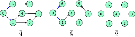
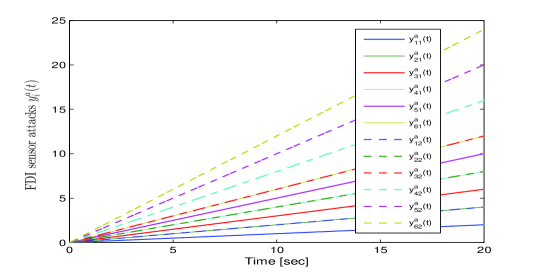
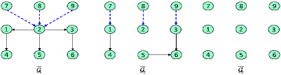
The unreliable directed communication topologies between the leader and the six followers are shown in Fig. 3, where only 𝒢¯1\bar{\mathcal{G}}_{1} has a directed spanning tree. It can be verified that Assumption 1 is satisfied. Besides, the linear multi-agent system suffers from unknown and unbounded FDI sensor attacks, i.e., yic(t)=yi(t)+ϕiayia(t),i𝒱.y^{c}_{i}(t)=y_{i}(t)+\phi^{a}_{i}y^{a}_{i}(t),i\in\mathcal{V}. Next, the control objective is to achieve resilient time-varying output formation tracking for multi-agent systems under FDI sensor attacks and unreliable digraphs.

Refer to caption
Figure 3: The unreliable communication topologies for a group of seven agents.

V-B Algorithm design and result

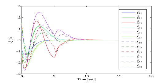
The proposed distributed leader estimator in (9) is performed under unreliable digraphs. We select the leader’s initial states as x0(0)=col(1,1)x_{0}(0)=\text{col}(1,-1), and the initial estimated states as ζi(0)=col(0.2,0.2;0.1,0;0.3,0.4;0.1,0.1;0.4,0.3;0.5,0.5)\zeta_{i}(0)=\text{col}(0.2,-0.2;-0.1,0;-0.3,0.4;0.1,-0.1;-0.4,0.3;-0.5,0.5). Based on certain calculations, one has that μ=1\mu=1, λm=0.7262\lambda_{m}=0.7262, σm=2.7071\sigma_{m}=2.7071. Further, the estimator gain matrix can be designed as K0=[0.0339 0.0524;0.01750.1517]K_{0}=[0.0339\ 0.0524;\ -0.0175\ -0.1517] by solving this optimization problem in (14)-(15), given R0=I2R_{0}=I_{2} and Q0=4I2Q_{0}=4I_{2}. The parameters κ0=2\kappa_{0}=2, τa=1\tau_{a}=1 and π=0.05\pi=0.05 are selected to satisfy (13) in Theorem 1. Then, the proposed reliable distributed leader estimator in (9) is performed, and the simulation result is depicted in Fig. 5. As can be observed, the leader’s state can be estimated for each follower exponentially.

The proposed resilient distributed control algorithms are performed against unbounded sensor attacks and unreliable digraphs.

Case 1: Resilient Output Formation Tracking with FDI Sensor Attacks and Unreliable Digraphs

In this part, these FDI sensor attacks are modeled by yia(t)=[0.1it;0.2it]y^{a}_{i}(t)=[0.1*i*t;0.2*i*t] shown in Fig. 4. As can be seen, Assumption 2 is verified. According to Theorem 2, the controller gain matrices are: K11=[84]K_{11}=[-8\ -4], K12=[7.52.75]K_{12}=[-7.5\ -2.75], K13=[82.3333]K_{13}=[-8\ -2.3333], K14=[78.7526.8755.5]K_{14}=[-78.75\ -26.875\ -5.5], K15=[9629.45.2]K_{15}=[-96\ -29.4\ -5.2], K16=[115.532.08335]K_{16}=[-115.5\ -32.0833\ -5]; K21=[212]K_{21}=[2\ -12], K22=[4.59]K_{22}=[4.5\ -9], K23=[68]K_{23}=[6\ -8], K24=[50.2574.25]K_{24}=[50.25\ -74.25], K25=[69.682.8]K_{25}=[69.6\ -82.8], K26=[90.591.5]K_{26}=[90.5\ -91.5]; and K31=[2 4]K_{31}=[2\ 4], K32=[3.5 3]K_{32}=[3.5\ 3], K33=[4.6667 2.6666]K_{33}=[4.6667\ 2.6666], K34=[43.5 25.75]K_{34}=[43.5\ 25.75], K35=[58.8 28.4]K_{35}=[58.8\ 28.4], K36=[76 31.1666]K_{36}=[76\ 31.1666]. By Proposition 1, the observer gain matrices are: L1=[2 1;0 1]L_{1}=[2\ 1;0\ 1], L2=[2 1;0 0.5]L_{2}=[2\ 1;0\ 0.5], L3=[2 1;0 0]L_{3}=[2\ 1;0\ 0], L4=[4.9998 0.9927;0.331 11.0002;2.6786 65.504]L_{4}=[4.9998\ 0.9927;-0.331\ 11.0002;-2.6786\ 65.504], L5=[4.9997 0.9930;0.4036 12.0003;3.6811 83.0059]L_{5}=[4.9997\ 0.9930;-0.4036\ 12.0003;-3.6811\ 83.0059], L6=[4.9995 0.9933;0.4811 13.0005;4.8797 102.5079]L_{6}=[4.9995\ 0.9933;-0.4811\ 13.0005;-4.8797\ 102.5079]; and Mi=[1 1.3;0.2 1]M_{i}=[-1\ 1.3;-0.2\ 1], i𝒱1i\in\mathcal{V}_{1}, Mi=[1 0.3;0.21]M_{i}=[-1\ 0.3;-0.2\ -1], i𝒱2i\in\mathcal{V}_{2}. The initial states xi(0)x_{i}(0) and x^i(0)\hat{x}_{i}(0) are randomly specified.

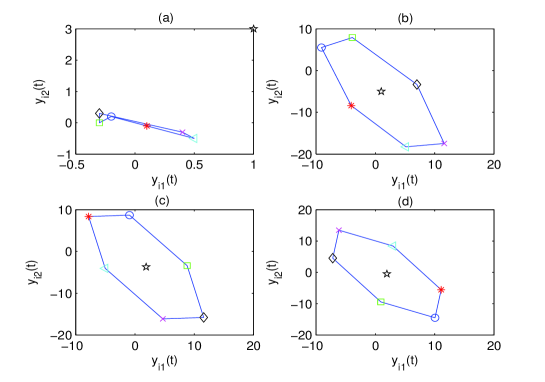
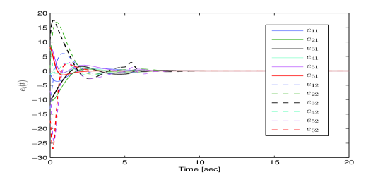
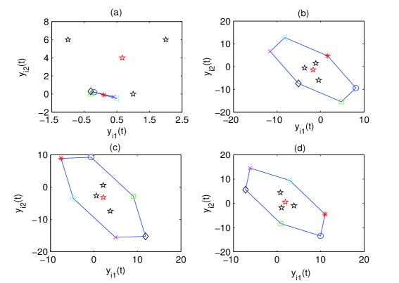
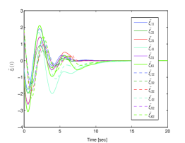
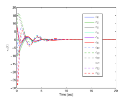
Next, the proposed resilient algorithm in (27)-(30) with (39) is performed, and the simulation results are shown in Figs. 5-7. Fig. 5 shows the leader-follower estimated error under unreliable digraphs. The output trajectories of all agents are shown in Fig. 6 for four different instants (t=0s, 8s, 15s, 20s). It can be seen in the presence of the FDI sensor attacks and unreliable communication, the six followers can rotate around the leader (black pentagram) that locates in the center of the time-varying formation. Moreover, Fig. 7 depicts the trajectories of output formation tracking errors ei(t)=yi(t)yhi(t)y0(t)e_{i}(t)=y_{i}(t)-y_{hi}(t)-y_{0}(t). From those figures, it is concluded that the time-varying output formation can be achieved under the FDI attacks and unreliable digraphs.

Refer to caption
Figure 4: Simulated FDI sensor attacks yia(t)=col(yi1a(t),yi2a(t)),i=1,,6y^{a}_{i}(t)=\text{col}(y^{a}_{i1}(t),y^{a}_{i2}(t)),i=1,\cdots,6.
Refer to caption
Figure 5: The trajectories of the leader-follower estimated error ξ~i=col(ξ~i1,ξ~i2)\tilde{\xi}_{i}=\text{col}(\tilde{\xi}_{i1},\tilde{\xi}_{i2}).
Refer to caption
Figure 6: The output trajectories of all agents yi=col(yi1,ey2)y_{i}=\text{col}(y_{i1},e_{y2}) under the sensor attacks and unreliable digraphs: (a) t=0s; (b) t=8s; (c) t=15s; and (d) t=20s.

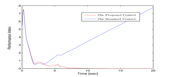
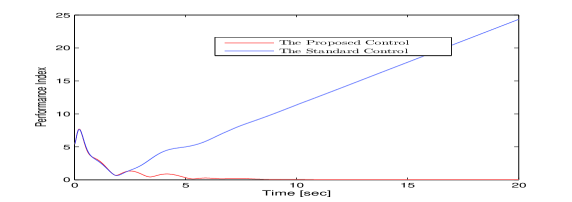
To show the resilient performance of the proposed algorithm, we compare our approach with the standard method, i.e., (27)-(30) without y^ia(t)\hat{y}^{a}_{i}(t) in (30) and fia(t)f^{a}_{i}(t) in (39). The performance index is: E(t)=16i=16ei2E(t)=\frac{1}{6}\sqrt{\sum_{i=1}^{6}\|e_{i}\|^{2}}, which is the average tracking error. The performance comparisons between the standard and the proposed resilient approaches are presented as depicted in Fig. 8. As can be observed, the proposed control method enables the zero-error tracking resilience against sensor attacks and unreliable digraphs, while the tracking error diverges under the standard method.

Refer to caption
Figure 7: The trajectories of the resilient time-varying output formation tracking ei=col(ei1,ei2)e_{i}=\text{col}(e_{i1},e_{i2}) under the sensor attacks and unreliable digraphs.
Refer to caption
Figure 8: The performance comparison between the standard and proposed methods.

Case 2: Resilient Output Containment-Formation Tracking with FDI Sensor Attacks and Unreliable Digraphs

The dynamics of the three leaders are described by x˙k(t)=[1,3;2,1]xk(t),yk(t)=[1,0;0,3]xk(t)\dot{x}_{k}(t)=[1,-3;2,-1]x_{k}(t),\ y_{k}(t)=[1,0;0,-3]x_{k}(t), k=7,8,9k=7,8,9, where xk(t)x_{k}(t), yk(t)y_{k}(t) are the state and output of the kkth leader, respectively. We select these three leaders’ initial states as x7(0)=col(1,0)x_{7}(0)=\text{col}(1,0), x8(0)=col(1,2)x_{8}(0)=\text{col}(-1,2), x9(0)=col(2,2)x_{9}(0)=\text{col}(2,-2). These unbounded FDI sensor attacks and the initial estimated states are given the same as those in Case 1. The unreliable digraphs between the leaders and the followers are provided in Fig. 9. The simulation results are depicted in Figs. 10-11. The state snapshots of three leaders, six followers and the convex combination of leaders are depicted in Fig. 10 for four different instants (t=0s, t=8s, t=15s and t=20s). It can be observed that 1) the states of the six followers can form a parallel hexagon, while rotating around the states of the three leaders; and 2) the states of these three leaders are time-varying and their convex combination can lie in the center of the parallel hexagon. That is, the desired time-varying output containment-formation tracking with multiple leaders has been achieved under FDI sensor attacks and unreliable digraphs. Fig. 11(a)-(c) shows the simulated results for ξ~i\tilde{\xi}_{i}, ei(t)=yi(t)yhi(t)k=79yk(t)e_{i}(t)=y_{i}(t)-y_{hi}(t)-\sum_{k=7}^{9}y_{k}(t), and performance comparison, respectively.

Refer to caption
Figure 9: The unreliable digraphs for a group of six followers and three leaders.
Refer to caption
Figure 10: The output trajectories of all agents yi=col(yi1,ey2)y_{i}=\text{col}(y_{i1},e_{y2}) in the presence of the FDI sensor attacks and unreliable digraphs under the proposed distributed algorithm in (58) together with (52): (a) t=0s; (b) t=8s; (c) t=15s; and (d) t=20s.

VI Conclusion

In this paper, we investigated the resilient time-varying output formation tracking problem of a heterogeneous linear multi-agent system under the unknown and unbounded FDI sensor attacks and unreliable digraphs. The new resilient distributed estimator-based control algorithms have been proposed to guarantee time-varying output formation tracking. Then, the proposed distributed design is extended to achieve time-varying output containment-formation tracking in the presence of FDI attacks and unreliable digraphs.

Refer to caption
(a) ξ~i\tilde{\xi}_{i}
Refer to caption
(b) eie_{i}
Refer to caption
(c) Performance index
Figure 11: Simulated results of time-varying output containment-formation tracking under the proposed distributed algorithm in (58) together with (52): (a) estimated tracking error ξ~i\tilde{\xi}_{i}; (b) time-varying output containment-formation tracking error eie_{i} and (c) performance comparisons between different methods.

References

  • [1] Z. Han, K. Guo, L. Xie, Z. Lin, “Integrated relative localization and leader-follower formation control,” Automatica, 64(1): 20–34, 2019.
  • [2] S. Du, X. Sun, M. Cao, W. Wang, “Pursuing an evader through cooperative relaying in agent surveillance networks,” Automatica, 83(9): 155–161, 2017.
  • [3] R. Zheng, Y. Liu, D. Sun, “Enclosing a target by nonholonomic mobile robots with bearing-only measurements,” Automatica, 53: 400–407, 2015.
  • [4] X. Dong, G. Hu, “Time-varying formation control for general linear multi-agent systems with switching directed topologies,” Automatica, 73(1): 47–55, 2016.
  • [5] X. Dong, G. Hu, “Time-varying formation tracking for linear multi-agent systems with multiple leaders,” IEEE Trans. Autom. Control, 62(2): 3658–3664, 2017.
  • [6] Y. Hua, X. Dong, G. Hu, Q. Li, Z. Ren, “Distributed time-varying output formation tracking for heterogeneous linear multi-agent systems with a nonautonomous leader of unknown input,” IEEE Trans. Autom. Control, 62(10): 4292–4299, 2019.
  • [7] W. Jiang, G. Wen, Z. Peng, T. Huang, A. Rahmani, “Fully distributed formation-containment control of heterogeneous linear multi-agent systems,” IEEE Trans. Autom. Control, 64(9): 3889–3896, 2019.
  • [8] Y. Wang, X. Liu, J. Xiao, Y. Shen, “Output formation-containment of interacted heterogeneous linear systems by distributed hybrid active control,” Automatica, 93(1): 26–32, 2018.
  • [9] S. Sundaram, C. N. Hadjicostis, “Distributed function calculation via linear iterative strategies in the presence of malicious agents,” IEEE Trans. on Automatic Control, 56(7), 1495–1508, 2011.
  • [10] F. Pasqualetti, A. Bicchi, F. Bullo, “Consensus computation in unreliable networks: a system theoretic approach,” IEEE Trans. on Automatic Control, 57(1), 90–104, 2012.
  • [11] T. Yucelen, W. M. Haddad, E. M. Feron, “Adaptive control architectures for mitigating sensor attacks in cyber-physical systems,” in IEEE. American control conference, pp. 1165-–1170, 2016.
  • [12] Z. Feng, G. Hu, G. Wen, “Distributed consensus tracking for multi-agent systems under two types of attacks,” Int. J. Robust. Nonlinear Control, 26(5) : 896–918, 2015.
  • [13] Z. Feng, G. Wen, G. Hu, “Distributed secure control for multi-agent systems under strategic attacks,” IEEE Trans. Cybern., 47(5): 1273–1284, 2017.
  • [14] Z. Feng, G. Hu, “Secure cooperative event-triggered control of linear multi-agent systems under DoS attacks,” IEEE Trans. Contr. Syst. Tech., 28(3): 741–752 2020.
  • [15] D. Zhang, L. Liu, G. Feng, “Consensus of heterogeneous linear multi-agent systems subject to aperiodic sampled-data and DoS attack,” IEEE Trans. Cybern., 49(4): 1501–1511, 2019.
  • [16] B. Chen, D. W. Ho, G. Hu, L. Yu, “Secure fusion estimation for bandwidth constrained cyber-physical systems under replay attacks,” IEEE Trans. Cybern., 48(6): 1862–1876, 2018.
  • [17] C. Deng, W. Che, P. Shi, “Cooperative fault-tolerant output regulation for multi-agent systems by distributed learning control approach,” IEEE Trans. Neural Netw. Learn. Syst., 31(11): 4831–4841, 2020.
  • [18] Z. Feng, G. Hu, “Connectivity-preserving flocking for networked Lagrange systems with time-varying actuator faults,” Automatica, 109(1): 1–10, 2019.
  • [19] C. Chen, F. L. Lewis, S. Xie, H. Modares, Z. Liu, S. Zuo, “Resilient adaptive and HH_{\infty} controls of multi-agent systems under sensor and actuator faults,” Automatica, 102: 19–26, 2019.
  • [20] H. Modares, B. Kiumarsi, F. L. Lewis, F. Ferrese, A. Davoudi, “Resilient and robust synchronization of multi-agent systems under attacks on sensors and actuators,” IEEE Trans. Cybern., 47(7): 1706–1718, 2020.
  • [21] S. Zuo, F. L. Lewis, A. Davoudi, “Resilient output containment of heterogeneous cooperative and adversarial multi-group systems,” IEEE Trans. Autom. Control, 65(7): 3104–3111, 2020.
  • [22] Y. Su, J. Huang, “Cooperative output regulation of linear multi-agent systems,” IEEE Trans. Autom. Control, 57(4): 1062–1066, 2012.
  • [23] Z. Li, M. Chen, Z. Ding, “Distributed adaptive controllers for cooperative output regulation of heterogeneous agents over directed graphs” Automatica, 68(1): 179–183, 2016.
  • [24] H. Cai, F. L. Lewis, G. Hu, J. Huang, “The adaptive distributed observer approach to the cooperative output regulation of linear multi-agent systems,” Automatica, 75(1): 299-–305, 2017.
  • [25] Z. Feng, G. Hu, W. Ren, W. E. Dixon, J. Mei, “Distributed coordination of multiple Euler-Lagrange systems,” IEEE Trans. Control Netw. Syst., 5(1): 55–66, 2018.
  • [26] Z. Li, Z. Duan. Cooperative control of multi-agent systems: a consensus region approach. CRC Press, 2014.
  • [27] F. L. Lewis, D. M. Dawson, C. T. Abdallah. Robot manipulator control: theory and practice. CRC Press, 2003.
  • [28] R. T. Rockafellar. Convex analysis. Princeton Press, NJ, USA, 2015.