Reshape: Adaptive Result-aware Skew Handling for Exploratory Analysis on Big Data
Abstract.
The process of data analysis, especially in GUI-based analytics systems, is highly exploratory. The user iteratively refines a workflow multiple times before arriving at the final workflow. In such an exploratory setting, it is valuable to the user if the initial results of the workflow are representative of the final answers so that the user can refine the workflow without waiting for the completion of its execution. Partitioning skew may lead to the production of misleading initial results during the execution. In this paper, we explore skew and its mitigation strategies from the perspective of the results shown to the user. We present a novel framework called Reshape that can adaptively handle partitioning skew in pipelined execution. Reshape employs a two-phase approach that transfers load in a fine-tuned manner to mitigate skew iteratively during execution, thus enabling it to handle changes in input-data distribution. Reshape has the ability to adaptively adjust skew-handling parameters, which reduces the technical burden on the users. Reshape supports a variety of operators such as HashJoin, Group-by, and Sort. We implemented Reshape on top of two big data engines, namely Amber and Flink, to demonstrate its generality and efficiency, and report an experimental evaluation using real and synthetic datasets.
1. Introduction
As information volumes in many applications become large, data analytics is becoming increasingly important. Data processing frameworks such as Hadoop (Apache Hadoop MapReduce, [n.d.]), Spark (APACHE Spark, [n.d.]), and Flink (APACHE Flink, [n.d.]) provide programming interfaces that are used by developers to code their data processing needs. GUI-based workflow systems such as Alteryx (Alteryx, [n.d.]), RapidMiner (RapidMiner, [n.d.]), Knime (Knime, [n.d.]), Einblick (Einblick, [n.d.]), and Texera (Wang et al., 2020) provide a GUI interface where the users can drag-and-drop operators and create a workflow as a directed acyclic graph (DAG). Once the data processing job is created, it is submitted to an engine that executes the job.
The process of data analysis, especially in GUI-based analytics systems, has two important characteristics. 1) Highly exploratory: The process of building a workflow can be very exploratory and iterative (Fisher et al., 2012; Xu et al., 2022; Vartak et al., [n.d.]). Often the user constructs an initial workflow and executes it to observe a few results. If they are not desirable, she terminates the current execution and revises the workflow. The user iteratively refines the workflow until finishing a final workflow to compute the results. As an example, Figure 1 shows a workflow at an intermediate step during the task of covid data analysis. It examines the relationship between the number of tweets containing the keyword covid and the number of Covid cases in 2020. The monthly details about the Covid cases are joined with tweets filtered on the covid keyword on the month column. The result is plotted as a visualization operator that shows a bar chart about the total count of tweets about Covid per month and a line chart about the total Covid cases per month. The analyst may observe the visualization and choose to continue refining the workflow to do analysis for specific US states. In the Texera system we are developing, we observe that the users refined a workflow about times on an average before reaching the final version. 2) Suitable for non-technical users: GUI-based workflow execution systems significantly lower the technical learning curve for its users, thus enabling non-IT domain experts to do data science projects without writing code. Such systems also try to minimize the requirements on users to know the technical details of workflow execution, so that the user can focus solely on the analytics task at hand.

In exploratory data analytics, it is vital for a user to see results quickly to allow her to identify problems in the analysis early and take corrective actions without waiting for the entire workflow to finish executing. Pipelined execution (Benoit et al., 2013) is a popular workflow execution model that can produce results quickly. In pipelined execution, an operator does not wait for its entire input data to be produced before processing the input and sending results to its downstream operators. For example, when the workflow in Figure 1 is executed using pipelined model, the HashJoin operator starts executing and producing results as soon as the Filter operator outputs initial results. The user can notice the initial results and make any changes, if needed. Pipelined execution is adopted by data-processing engines such as Flink (APACHE Flink, [n.d.]), Samza (apache-samza, [n.d.]), and Storm (ApacheStorm, [n.d.]).
As data volumes in these systems increase, it is indispensable to do parallel processing, in which data is partitioned and processed by multiple computation units in parallel. Data partitioning, either using hash partitioning or range partitioning, often results in skew. As an example, the HashJoin operator in Figure 1 receives hash partitioned inputs from the two upstream operators. Although the hash function allots the same number of months to each join worker, load imbalance still exists because of different numbers of tweets for those months. It is well known that partitioning skew adversely affects the efficiency of engines as it increases the processing time and reduces the throughput (DeWitt et al., 1992; Kwon et al., 2012).
The problem of partitioning skew has been extensively studied in the literature, mainly from the perspective of increasing the end-to-end performance. However, there is little research on the following important problem:
In exploratory data analytics, how to consider the results shown to the user when mitigating skew?
In exploratory data analysis, it is valuable to the analyst if the initial results are representative of the final results because they allow her to identify issues early and make necessary changes. Partitioning skew may lead to the production of misleading results during the execution. Let us consider the production rate of October and December tuples from the HashJoin operator in the running example. Assume that the HashJoin operator is the bottleneck of the execution, and its workers receive input at an equal or higher rate than they can process. Although there are more December tuples than October, their production rates are similar because the total amounts of data received by and are different (details in Section 3). Thus, the bar chart shows similar heights for October and December bars till completes processing, whereas the December bar is almost four times taller than the October bar in the final result. In this paper, we explore partitioning skew mitigation in the setting of exploratory data analysis and analyze the effect of mitigation strategies on the results shown to the user.
A common solution to handle partitioning skew at an operator is blocking the partitioning of its input data till the entire input data is produced by its upstream operator (sparkaqewebsite, [n.d.]; DeWitt et al., 1992; Vitorovic et al., 2016; Chen et al., 2015; Abdelhamid et al., 2020) and then sampling the input data to create an optimal partitioning function. For example, in Figure 1, the HashJoin operator waits for the Filter operator to completely finish. Then, the output of the Filter operator is sampled to create an optimal partitioning function to send data to the HashJoin operator. Such blocking is not allowed in pipelined execution which makes these solutions infeasible in pipelined execution setting. Even temporarily blocking the partitioning till a small percentage of input (e.g., 1% (Rödiger et al., 2016)) is collected for sampling can result in a long delay if there is an expensive upstream operator.
A different solution applicable to the pipelined execution setting is to detect the overloaded workers of an operator at runtime and transfer the processing of a few keys of the overloaded worker to a more available worker. For example, is detected to be overloaded at runtime and the processing of June tuples is transferred to . However, this transfer has little effect on the results shown to the user (details in Section 3). In order to show representative initial results, the data of December has to be split between and . Thus, these two approaches of transferring load from to have different impacts on the initial results shown to the user.
In this paper, we analyze the effect of different skew mitigation strategies on the results shown to the user and present a novel skew handling framework called Reshape that adaptively handles skew in a pipelined execution setting. Reshape monitors the workload metrics of the workers and adapts the partitioning logic to transfer load whenever it observes a skew. These modifications can be done multiple times as the input distribution changes (Beitzel et al., 2004; Kulkarni et al., 2011) or if earlier modifications did not fully mitigate the skew. The command to adapt the partitioning logic is sent from the controller to the workers using low latency control messages that are supported in various engines such as Flink, Chi (Mai et al., 2018), and Amber (Kumar et al., 2020).
We make the following contributions. (1) Analysis of the impact of mitigation on the shown results: We present different approaches of skew mitigation and analyze their impact on the results shown to the user. (Section 3). (2) Automatic adjustment of the skew detection threshold: We present a way to dynamically adjust the skew detection threshold to reduce the number of iterations of mitigation to minimize the technical burden on the user (Section 4). (3) Applicability to multiple operators: Since a data analysis workflow can contain many operators that are susceptible to partitioning skew, we generalize Reshape to multiple operators such as HashJoin, Group-by, and Sort, and discuss challenges related to state migration (Section 5). (4) Generalization to broader settings: We consider settings such as high state-migration time and multiple helper workers for an overloaded worker and discuss how Reshape can be extended in these settings (Section 6). (5) Experimental evaluation: We present the implementation of Reshape on top of two big-data engines, namely Amber and Flink, to show the generality of this approach. We report an experimental evaluation using real and synthetic datasets on large computing clusters (Section 7).
1.1. Related work
There have been extensive studies about skew handling in two major execution paradigms in big data engines – batch execution and pipelined execution. Batch-execution systems such as MapReduce (Apache Hadoop MapReduce, [n.d.]) and Spark (APACHE Spark, [n.d.]) materialize complete input data before partitioning it across workers. Pipelined-execution systems such as Flink (APACHE Flink, [n.d.]), Storm (ApacheStorm, [n.d.]) and Amber (Kumar et al., 2020) send input tuples to a receiving worker immediately after they are available. The complete input is not known to the operator in pipelined execution, which makes skew handling more challenging.
Skew handling in batch execution. A static technique is to sample and obtain the distribution of complete input data and use it to partition data in a way that avoids skew (sparkaqewebsite, [n.d.]; DeWitt et al., 1992; Vitorovic et al., 2016; Chen et al., 2015; Abdelhamid et al., 2020). Adaptive skew-handling techniques adapt their decisions to changing runtime conditions and mitigate skew in multiple iterations. For instance, SkewTune (Kwon et al., 2012) and Hurricane (Bindschaedler et al., 2018) handle skew adaptively. That is, upon detecting skew, SkewTune stops the executing workers, re-partitions the materialized input, and starts new workers to process the partitions. Hurricane clones overburdened workers and uses a special storage that allows fine-grained data access to the original and cloned workers in parallel. Hurricane can split the processing of a key over multiple workers and thus has a fine load-transfer granularity. SkewTune cannot split the processing of a key.
Static skew handling in pipelined execution. Flow-Join (Rödiger et al., 2016) avoids skew in a HashJoin operator. It samples the first 1% of input data of the operator to decide the overloaded keys and does a broadcast join for the overloaded keys. Since it makes the decision based on an initial portion of the input, it cannot handle skew if the input distribution changes multiple times during the execution. Partial key grouping (PKG) (Nasir et al., 2015, 2016) uses multiple pre-defined partitioning functions. It results in multiple candidate workers sharing the processing of the same key. Since the partitioning logic is static, a worker may process multiple skewed keys, which makes it more burdened than other workers. PKG cannot be used to handle skew in operators such as Sort and Median.
Adaptive skew handling in pipelined execution. Flux (Shah et al., 2003) divides the input into many pre-defined mini-partitions that can be transferred between workers to mitigate skew. Thus, the load-transfer granularity is fixed and pre-determined. Also, it cannot split the load of a single overloaded key to multiple workers. Another adaptive technique minimizes the input load on workers that compute theta joins by dynamically changing the replication factor for data partitions (Elseidy et al., 2014). This approach uses random partitioning schemes such as round-robin and hence is not prone to partitioning skew. Reshape handles skew adaptively over multiple iterations. It determines the keys to be transferred dynamically and allows an overloaded key to be split over multiple workers for mitigation.
2. Reshape: Overview
We use Figure 2 to give an overview of Reshape.

2.1. Skew detection
During the execution of an operator, the controller periodically collects workload metrics from the workers of the operator to detect skew (Figure 2(a)). There are different metrics that can represent the workload on a worker such as CPU usage, memory usage and unprocessed data queue size (Bindschaedler et al., 2018; Fernandez et al., 2013). Skew handling in Reshape is independent of the choice of workload metric, and we choose unprocessed queue size as a metric in this paper. We choose this metric because the results seen by the analyst depend on the future results produced by a worker, which in turn depend on the content of its unprocessed data queue. We refer to a computationally overburdened worker as a skewed worker and workers that share the load as its helper workers.
Skew test. Given two workers of the same operator, say and , the controller performs a skew test to determine whether is a helper candidate for . The skew test uses the following inequalities to check if is computationally burdened and the workload gap between and is big enough:
| (1) |
| (2) |
where and are threshold parameters and is the workload on a worker .
Helper workers selection. The skew tests may yield multiple helper candidates for . For simplicity, we assume till Section 5 that one helper worker is assigned per skewed worker. In Section 6, we generalize the discussions by considering multiple helpers per skewed worker. The controller chooses the helper candidate with the lowest workload that has not been assigned to any other overloaded worker as the helper of . In our discussions forward, we use and to refer to a skewed worker and its chosen helper worker respectively.
2.2. Skew mitigation
Suppose the skewed worker and its helper have been handling input partitions and , respectively (Figure 2(a)). Reshape transfers a fraction of the future input of to to reduce the load on . Here future input refers to the data input that is supposed to be received by a worker but has not yet been sent by the previous operator. The controller notifies about the part p of partition that will be shared with to reduce the load of (Figure 2(b)). The downstream results shown to the user have a role to play in deciding p, which will be discussed in Section 3. Worker sends to its state information corresponding to the partition p (Figure 2(c)). Details about state-migration strategies are in Section 5. We assume the state migration time to be small till Section 5. In Section 6, we consider the general case where the state-migration time can be significant. Worker saves the state information and sends an ack message to , which then notifies the controller (Figure 2(d)). The controller changes the partitioning logic at the previous operator (Figure 2(e,f)).
Fault Tolerance. The Reshape framework supports the fault tolerance mechanism of the Flink engine (Carbone et al., 2015) that checkpoints the states of the workers periodically. During checkpointing, a checkpoint marker is propagated downstream from the source operators. When an operator receives the marker from all its upstream operators, it takes a checkpoint which saves the current states of the workers of the operator. Every checkpoint has the information about the current partitioning logic at the workers. If checkpointing occurs during state migration, then the skewed worker additionally forwards the checkpoint marker to each of its helper workers. A helper worker needs to wait for the checkpoint marker from its corresponding skewed worker. Since the skewed workers and the helper workers are two disjoint sets of workers, there is no cyclic dependency in marker propagation and the checkpointing process successfully terminates. During recovery, the workers restore their states from the most recent checkpoint and then continue the execution.
3. Result-aware Load transfer
After helper workers are selected for the skewed workers, the load needs to be transferred from the skewed workers to the corresponding helper workers. In Section 3.1, we consider the different approaches of load transfer between workers and analyze their impact on the results shown to the user. Unlike other skew handling approaches that focus on evenly dividing the future incoming load among the workers, Reshape has an extra phase of load transfer at the beginning that removes the existing load imbalance between the workers. In Section 3.2, we discuss these two phases of load transfer and the significance of the first phase.
3.1. Mitigation impact on user results
There are broadly two approaches to transfer the load from a skewed worker to its helper worker. We use the probe input of the HashJoin operator in Figure 1 (from the Filter operator) as an example to explain the concepts in this section. It is assumed that the build phase of the join has finished. Suppose Reshape detects and as the skewed workers in the running example and and are their corresponding helpers, respectively. The load-transfer approaches are implemented by changing the partitioning logic at the Filter operator and affects the future tuples going into the HashJoin operator.
1. Split by keys (SBK). In this approach, the keys in the partition of the skewed worker are split into two disjoint sets, say and . The future tuples belonging to are redirected to the helper worker, while tuples belonging to continue to be sent to the skewed worker. For example, the partition of the skewed worker is divided into = {December} and = {June}, and the future June tuples are sent to , while December tuples continue to go to .
2. Split by records (SBR). In this approach, the records of the keys in the partition of the skewed worker are split between the skewed and the helper worker. The ratio of the split decides the amount of load transferred to the helper worker. For example, if the Filter operator needs to redirect of the input to , then it redirects tuples out of every tuples in ’s partition to .
Impact of the two approaches on user results. The two load transfer approaches have their own advantages and limitations. For example, SBK incurs an extra overhead compared to SBR because SBK requires the workers to store the distribution of workload per key. On the other hand, SBR may require transfer of a larger state size compared to SBK, if all the keys of a skewed worker are shared with the helper. There are existing works in literature that address these concerns (Metwally et al., 2005; Rödiger et al., 2016; Yan et al., 2013; Gufler et al., 2012; Monte et al., 2020; Hoffmann et al., 2019). In the remainder of this subsection, we compare these two approaches from the perspective of their effects on the results shown to the user.
a) Representative initial results. As discussed before, it is valuable to the user if the initial results are representative of the final results. Partitioning skew may lead to the production of misleading results during the execution as shown next. Let us consider the bar chart visualization for October and December in the running example. The total count of December tweets, according to Figure 1(c), is about four times that of October tweets, i.e., the December bar is about four times longer than the October bar in the final visualization. Assume that the join operator is the bottleneck of the execution, and its workers receive input at an equal or higher rate than what they can process. Also assume that the processing speeds of the workers of HashJoin are the same, say per second. produces October tuples and produces December tuples per second in the unmitigated case (Figure 3(a)). The rate of production of October and December tuples are similar because the total amount of data received by and are different. The bar chart shows similar heights for October and December bars in the unmitigated case till completes its processing.

When SBK is used to mitigate the skew, the processing of June tuples is transferred to (Figure 3(b)). However, this transfer has little effect on the results shown to the user. The production rates of October and December after the transfer are and respectively. That is, the heights of the December and October bars are still about the same, which is not representative of the final results.
SBR has more flexibility for transferring load than SBK because SBR can split the tuples of a key over multiple workers. It leads to more representative initial results than SBK as shown next. The processing of December and June tuples can be split between and . For simplicity of calculation, we assume that only December tuples are shared with . Since December tuples are now processed by two workers instead of one, the speed of production of these tuples increases. In order to make the future workloads of and similar, SBR redirects of the input of to , which increases the total percentage load on to and decreases that on to . This is implemented by redirecting December tuples out of every tuples in ’s partition to . The production rates of October tuples after the transfer is . The December tuples are produced by and . The production rate of December by is and by is , which results in a total of approximately . Thus, using SBR leads to a more representative production ratio of December to October tuples of about , which is similar to the actual ratio of .

b) Preserving order of tuples. If the tuples of a key being input into an operator are in a particular order and they need to be processed in that order, then SBK is the suitable approach because it enforces a processing order by restricting the processing of the tuples of a key to a single worker at a time. If the processing of a key needs to be transferred to another worker, the migration can be synchronized using techniques such as pause and resume (Armbrust et al., 2018; Carbone et al., 2017; Shah et al., 2003) or markers (Elseidy et al., 2014) (details in Section 5) so that the tuples are processed in order. In contrast, SBR distributes the tuples of a key over multiple workers to be processed simultaneously, which may cause them to be processed out of order. Consider the following example where an out-of-order processing of the tuples of a key is not desirable. Let us slightly modify the visualization operator in the running example to plot a line chart that shows daily count of covid related tweets. The daily count for each month is plotted as a separate line in the line chart. Figure 4 shows the plot for December in the line chart. Applications may want to show such plots as a continuous line with no breaks, starting from day 1 and extending towards increasing dates as execution progresses, for user experience purposes (Clo, 2018). In order to achieve this, the tuples of a month input into the HashJoin operator are sorted in the increasing order of date. It is expected that HashJoin produces tuples sorted by date, which can be consumed by the visualization operator to create a continuous plot.
SBK assures that the December key is processed by only one worker at a time. Thus, it preserves the order of December tuples in the output sent to the visualization operator (Figure 4(a)). When SBR is used, the December tuples are split between and . In the example shown in Figure 4(b), the Filter operator starts partitioning December tuples by SBR when the tuples around the of December are being produced by the Filter operator. Consequently, starts receiving the tuples from the date of the December and above. As and concurrently process data, the visualization operator receives the tuples out of order, resulting in broken line chart plots as shown in the figure.
In conclusion, SBR allows more flexibility and enables the production of representative initial results than SBK, but SBR does not preserve the order of tuples. Thus, SBR can be chosen unless there exists a downstream operator that imposes some requirement over the input order of the tuples. Such operators can be found at the workflow compilation stage. The operators before such an operator in the workflow can adopt SBK.
3.2. Extra phase in load transfer
The goal of skew mitigation is to use one of the two approaches to transfer the load from the skewed worker to the helper worker in such a way that both workers have a similar workload for the rest of the execution. The skew handling works in literature usually have a single phase of load transfer that focuses on splitting the incoming input such that the workers receive similar load in future. Reshape has an extra phase of load transfer at the beginning that removes the existing load imbalance between the workers. We first give an overview of the two phases in Reshape, and explain the significance of the first phase.
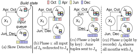
First Phase. After the detection of skew (Figure 5(a)), the controller starts the first phase of load transfer. The first phase lets the helper “catch up” quickly with the skewed worker. One implementation of the partitioning logic in the first phase at the Filter operator is that it sends all future tuples of to (Figure 5(b)). Note that will continue to process the data in its queue. An alternative implementation is to send only a portion of ’s partition, such as the December data, to . This alternative reduces the amount of state transfer, but it will take longer time for to catch up with .
Second Phase. Once the queue sizes of the two workers become similar, the controller starts the second phase. Its goal is to modify the partitioning logic at the Filter operator to redirect part of the future input of in such a way that both the workers receive a comparable workload. In order to do this, first the incoming workload of the workers needs to be estimated. A sample of workloads needs to be collected to estimate the future workload of the workers (Ramakrishnan et al., 2012; Chen et al., 2015; Yan et al., 2013; Gufler et al., 2012) using a prediction function . Reshape can use the sample from the recent history collected during the current execution (Kim et al., 2016; Shen et al., 2011). If historical data is available, it can complement the recent data and improve the prediction accuracy (Garraghan et al., 2015; Popescu et al., 2012).
To simplify the discussion of the second phase, we make the following assumptions:
-
•
The two workers receive data at constant rates.
-
•
We have a perfect estimator to accurately predict the incoming data workload on the workers.
In Section 4 we will relax these two assumptions. In Figure 1(c), the original load ratio of to is . SBK cannot handle the skew between and . The approach transfers the June month to (Figure 5(c1)), which does not mitigate the skew. However, SBR can redirect of the input of to , which mitigates the skew by increasing the percentage load on to and decreasing the percentage load on to . An example where SBK can mitigate the skew is the case of skew between the skewed worker and its helper . SBK can transfer the processing of May to , which brings the two workers to a similar workload. Specifically, the percentage load on increases to and that on decreases to .
It should be noted that two phases do not mean that the state transfer has to be done twice necessarily. There are implementations where the state transfer during the first phase is enough and the second phase does not require another state transfer. For example, in SBR, the state of all keys are sent to in the first phase, and there is no state migration needed for the second phase.

Significance of the first phase. Reshape has an extra phase for two reasons. First, it gives some immediate respite to the skewed worker and avoids imminent risks of the skewed worker going out of computing resources, invoking back-pressure (Backpressure, [n.d.]) etc. Second, it may allow the user to see the representative results earlier compared to the case where there is only one phase. Figure 6 illustrates this idea. For simplicity of calculation, we assume that processes October and processes December only. Notice that December tuples are almost four times the tuples of October (Figure 1(c)). Suppose the HashJoin operator receives October and December tuples every second and the skew is detected when the unprocessed queue sizes of and are and , respectively. Figure 6(a) shows the case where there exists a first phase. Suppose the first phase redirects all December tuples to . In seconds, receives December and October tuples and catches up with the queue of . After this, the second phase starts and redirects out of every December tuples to . Assuming the workers process tuples at similar rates, the bar charts show the October and December tuples count shown to the user as the workers process more data. When the workers have processed tuples each, the bar chart shows tuples for both months. After that the effect of first phase starts. When both workers have processed tuples each, the bar chart shows tuples for October and tuples for December, which is representative of the ratio of October to December tuples in the input data. Figure 6(b) shows the case where there is no first phase. After detection of skew, the second phase starts and redirects out of every December tuples to . In this case, even after both the workers have processed tuples each, the bar chart shows tuples for October and tuples for December. The ratio gradually moves towards the actual ratio of between October to December tuples.
4. Adaptive Skew Handling
In the previous section, we assumed that data arrives at constant rates to the workers and the second phase has a perfect estimator. In this section, we study the case when these assumptions are not true. In particular, variable patterns in incoming data rates and an imperfect estimator can result in erroneous workload predictions. Consequently, the second phase may not be able to keep the workload of the skewed and helper workers at a similar level. Thus, the controller may start another iteration of mitigation. Since, each iteration may incur an overhead, such as state transfer, we should try to make better workload predictions so that the number of iterations is reduced. We show that the workflow prediction accuracy depends on the skew detection threshold (Sections 4.1 and 4.2). In order to reduce the technical burden on the user to fix an appropriate , we develop a method to adaptively adjust to make better workload predictions (Section 4.3).
4.1. Load reduction from mitigation
We measure the load reduction () from mitigation as the difference in the maximum input size received by a skewed worker and its helper without and with mitigation. Formally, let and represent the skewed worker and the helper worker, respectively. The load reduction is defined as:
| (3) |
where is the size of the total input received by a worker during the entire execution.
In Figure 7, represents the difference in the total input sizes of and in the unmitigated case. When mitigation is done, due to workload estimation errors, the second phase may not be able to redirect the precise amount of data to keep the workloads of and at a similar level. In Figure 7(a), less than tuples of are redirected to . Thus, receives more total input than and the load reduction is less than . Similarly, in Figure 7(b), more than tuples of are redirected to . As a result, the load reduction is again less than . The ideal mitigation, shown in Figure 7(c), makes the total input of the two workers equal so that they finish around the same time. In particular, tuples of are sent to , which is the maximum load reduction () that can be achieved.

4.2. Impact of on load reduction
In this subsection, we discuss how the load reduction is affected by the value of at which the mitigation starts. Assume that the operator can have only one iteration of mitigation consisting of two phases. If the second phase uses a perfect estimator and the incoming data rates are constant, as assumed in Section 3, then the maximum load reduction of can be achieved. That is:
| (4) |
where and are the load reduction resulting from the first phase and second phase, respectively.
In general, the workloads estimations have errors (Chaudhuri et al., 1998; Ramakrishnan et al., 2012; Chen et al., 2015; Yan et al., 2013; Gufler et al., 2012). These errors can cause the second phase to redirect less or more than the ideal amount of tuples (Figure 7(a,b)). In other words, the load reduction from the second phase depends on the accuracy of workload estimation. The workload estimation accuracy depends on as shown next. If increases, then it takes a longer time for the workload difference of and to reach , resulting in a higher sample size. Suppose the estimation accuracy increases as the sample size increases. Then a higher means that the system makes a more accurate workload estimation. Thus, the total load reduction can be computed as the following:
| (5) |
where is a function representing the error in the estimation of the future workloads. As increases, decreases.
The above analysis shows that a higher results in a higher load reduction. However, setting to an arbitrarily high value means that the system waits a long time before starting the mitigation. Consequently, there may not be enough future input left to mitigate the skew completely. Thus the value of should be chosen properly to achieve a balance between a high estimation accuracy and waiting so long that the opportunity to mitigate skew is lost. This is a classic exploration-exploitation dilemma (Auer et al., 2002).

Figure 8(a) shows the relationship between and load reduction. A small results in a small load reduction because of a high estimation error. As increases, decreases and load reduction increases. The load reduction cannot exceed . However, the load reduction does not remain at as further increases, as shown next. Suppose and are to receive and tuples in total, respectively. Figure 8(b) shows the time when they have received and tuples respectively. At this time, the remaining tuples of can be redirected to to achieve the maximum load reduction of (). The difference in the workloads of the workers at this time is denoted by . After , the load reduction continues to decrease because there are not enough future tuples left. Ultimately, at , the load reduction becomes .
4.3. Adaptive mitigation iterations
When the workloads of and diverge due to workload estimation errors, the controller may start another mitigation iteration. Section 4.3.1 discusses how multiple iterations of mitigation are performed. In the previous subsection, we saw that should be chosen appropriately to maintain a balance between workload estimation accuracy and a long delay in the start of mitigation. Section 4.3.2 shows how to autotune adaptively to make better workload estimations, rather than asking the user to supply an appropriate value of .
4.3.1. Multiple iterations of mitigation
Figure 9 shows an example timeline of two successive iterations of mitigation. The first iteration starts at when the difference of the workloads of and exceeds . Their workloads are brought to a similar level at . Then, the second phase starts. Due to workload estimation errors, the second phase redirects less than the ideal amount of tuples. Thus, the workload of gradually becomes greater than . At , their workload difference exceeds and the second iteration starts.

A question is how to decide the time interval from which the sample is used to do prediction (Xiao et al., 2013; Di et al., 2012). Figure 9 shows an example that uses the sample collected since the last time when and had a similar load. Specifically, at , the second phase of the first iteration uses the sample collected since . The second phase of the second iteration uses the sample collected since .
4.3.2. Dynamically adjusting
A low value of causes high errors in workload estimation due to a small sample size, which in turn results in more mitigation iterations. On the other hand, a high may start the mitigation too late when there are not enough future tuples to mitigate the skew. Rather than using a fixed user-provided value of , which may be too low or too high, we adaptively adjust ’s value during execution to make better workload predictions, reduce the number of iterations, and achieve higher load reduction.
In Section 3, we introduced an estimation function that uses a workload sample to estimate future workloads. Let denote the standard error of estimation (Prediction interval, [n.d.]), which is a measure of predicted error in workload estimation. For example, the standard error for mean-model (Statistical forecasting, [n.d.]; Prediction interval, [n.d.]) estimator is , where is the sample standard deviation and is the sample size. As mentioned in Section 4.2, decreases as increases. We want to be in a user-defined range , where and are the lower and upper limits, respectively. In particular, when , we assume the error is too high and will lead to a low load reduction. Similarly, when , the error is low enough to make a good estimation.
The controller keeps track of and adaptively adjusts in order to move towards the range. Algorithm 1 describes the process of adjusting . For a worker , let represent the current workload and represent the workload predicted by . The controller periodically collects the current workload metrics from the workers (line 1) and adds them to the existing sample (line 1). The function uses the workload sample to predict future workloads and outputs in the prediction (line 1). Once is obtained, can be adjusted.
Increasing . The need to increase arises when the workers and pass the skew-test (Section 2.1), but . This means that a higher sample size is needed to lower . At this point, the mitigation is started and an increased is chosen for the next iteration to achieve a smaller . The threshold should be cautiously increased so as to not set it to a very high value (Section 4.2).
Decreasing . Now consider the case where and do not pass the skew-test because their workload difference is less than , but . This means that is low and the sample size is big enough to yield a good accuracy. If we wait for the workload difference to reach , there may not be enough data left to mitigate the skew. Thus, is decreased to the current workload difference () and mitigation starts right away, thus yielding a higher load reduction.
5. Reshape on more operators
Till now we used the running example of skew in the probe input of HashJoin. A data analysis workflow can contain many operators that are susceptible to partitioning skew such as sort and group by. In this section, we generalize Reshape to a broader set of operators. Specifically, we formalize the concept of “operator state mutability” in Section 5.1. In Section 5.2, we discuss the impact of state mutability on state migration. In Sections 5.3 and 5.4, we use the load-transfer approaches described in Section 3 to handle skew in mutable-state operators. We discuss a state migration challenge when using the “split by records” approach and explain how to handle it.
5.1. Mutability of operator states
In this subsection, we define two types of operator states, namely immutable state and mutable state. When an operator receives input partitioned by keys, the state information of keys is stored in the operator as keyed states (Carbone et al., 2017). Each keyed state is a mapping of type
where is a single key or a set or range of keys, and is information associated with the . For example, in HashJoin, each join key is a , and the list of build tuples with the key is the corresponding . Similarly, in a hash-based implementation of group-by, each individual group is a , and the aggregated value for the group is the corresponding . In a range-partitioned sort operator, a range of keys is a , and the sorted list of tuples in the range is the corresponding . In the rest of this section, for simplicity, we use the term “state” to refer to “keyed state.”
An input tuple uses the state associated with the of the key of the tuple. If the of this cannot change, we say the state is immutable; otherwise, it is called mutable. For example, the processing of a probe tuple in HashJoin does not modify the list of build tuples for its key. Such operators whose states are immutable are called immutable-state operators. On the other hand, an input tuple to sort is added to the sorted list associated with its (range of keys), thus it modifies the state. Such operators that have a mutable state are called mutable-state operators.
Notice that the execution of an operator can have more than one phase. For instance, a HashJoin operator has two phases, namely the build phase and the probe phase. The concept of mutability is with respect to a specific phase of the operator. In HashJoin, the states in the build phase are mutable, while the states in the probe phase are immutable. Reshape is applicable to a specific phase, and its state migration depends on the mutability of the phase. Table 1 shows a few examples of immutable-state and mutable-state operators.
| Immutable-state operator | HashJoin (Probe phase), HB Set Difference (Probe phase), HB Set Intersection (Probe phase) |
| Mutable-state operator | HashJoin (Build phase), HB Group-by, RB Sort, HB Set Difference (Build phase), HB Set Intersection (Build phase), HB Set Union |
5.2. Impact of mutability on state migration
Figure 10 shows how to handle state migration for operators when using the two load-transfer approaches discussed in Section 3.

The state-migration process for immutable-state operators, as shown in branch (a) in Figure 10, involves replicating the skewed worker’s states at the helper, followed by a change in the partitioning logic. Thus, the tuples redirected from the skewed worker to the helper can use the state of their at the latter. In contrast, the state-migration process is more challenging for mutable-state operators (branch (b)) because it is difficult to synchronize the state transfer and change of partitioning logic for a mutable state (Mai et al., 2018). State-migration strategies that focus on such synchronization exist in the literature and will be briefly discussed in Section 5.3. As we show in Section 5.4, such a synchronization is not always possible. Next, we discuss how to do state migration when using the two load-transfer approaches in mutable-state operators.
5.3. Mutable-state operators: split by keys
The SBK approach offloads the processing of certain keys in the skewed worker partition to the helper. Consider a group-by operator that receives covid related tweets and aggregates the count of tweets per month. The skewed worker offloads the processing of a month (say, June) to the helper. There needs to be a synchronization between state transfer and change of partitioning logic so that the redirected June tuples arriving at the helper use the state formed from all June tuples received till then. In the case of group-by, this state is the count of all June tuples received by the operator. Existing work on state-migration strategies focuses on this synchronization. A simple way to do this synchronization is to pause the execution, migrate the state, and then resume the execution (Armbrust et al., 2018; Carbone et al., 2017; Shah et al., 2003). A drawback of this approach is that pausing multiple times for each iteration may be a significant overhead. Another strategy is to use markers (Elseidy et al., 2014). The workers of the previous operator emit markers when they change the partitioning logic. When the markers from all the previous workers are received by the skewed and helper workers, the state can be safely migrated. Thus, skew handling in mutable-state operators using the “split by keys” approach can be safely done by using one of these state-migration strategies (branch (b1) in Figure 10).
5.4. Mutable-state operators: split by records
In this subsection, we use the SBR approach in mutable-state operators (branch (b2) in Figure 10). We show that the synchronization between state transfer and change of partitioning logic is not possible when using this approach and discuss its effects. Consider a sort operator with three workers, namely , , and , which receive range-partitioned inputs. The ranges assigned to the three workers are , , and . As shown in Figure 11(a), is skewed and is its helper. The controller asks the previous operator to change its partitioning logic and send the tuples in to both and (Figures 11(b,c)). The synchronization of state migration and change of partitioning logic by the aforementioned state-migration strategies relies on an assumption that, at any given time, the partitioning logic sends tuples of a particular to a single worker only. When the tuples of are sent to both and , this assumption is no longer valid. Worker saves the tuples from the range in a separate sorted list (Figure 11(d)). Such a scenario where the of a is split between workers is referred to as a scattered state.

This scattered state needs to be merged before outputting the results to the next operator. Now we explain a way to resolve the scattered state problem. When a worker of the previous operator finishes sending all its data, it notifies the sort workers by sending an END marker (Figure 11(d)). When receives END markers from all the previous workers, it transfers its tuples in the range to the correct destination of those tuples, i.e., (Figure 11(e,f)), thus merging the scattered states for the range.
We specify sufficient conditions for a mutable-state operator to be able to resolve the scattered state issue. The above approach of merging the scattered parts is suited for blocking operators such as group-by and sort, which produce output only after processing all the input data. Thus, the above approach can be used by mutable-state operators if they can 1) combine the scattered parts of the state to create the final state, and 2) block outputting the results till the scattered parts of the state have been combined.
6. Reshape in Broader Settings
Our discussion about Reshape so far is based on several assumptions in Section 2 for simplification. Next we relax these assumptions.
6.1. High state-migration time
The state-migration time is assumed to be small till now. In this subsection, we study the case where this time could be significant.
Precondition for skew mitigation. In the discussion in Section 2, state migration is started immediately after skew detection. If the time to migrate state is more than the time left in the execution, the state migration is futile. Thus, the controller checks if the estimated state-migration time is less than the estimated time left in the execution and only then proceeds with state migration. The state-migration time can be estimated based on factors such as state-size and serialization cost (Yun et al., 2020; Ding et al., 2015). The time left in the execution can be estimated by monitoring the input data remaining to be processed and the processing speed (Kwon et al., 2012) or by using the historical data (Gupta et al., 2008).
Dynamic adaptation of . Suppose the adapted value of output by Algorithm 1 to be used in the next iteration is . The discussion in Section 4.3.2 assumes that the load transfer begins when the workload difference is around . This is possible only when the state-migration time is small. When the time is significant, the load transfer will start when the workload difference becomes considerably greater than . In order to start the load transfer at (as assumed by Section 4.3.2), the skew has to be detected earlier. Thus, we adjust the skew detection threshold to , which is less than , such that the state migration starts when the workload difference is and ends when the workload difference is (Figure 12).

Formally, suppose is the number of tuples processed by the operator per unit time, is the estimated state-migration time, and and are the predicted workload percentages of and , respectively. The estimated difference in the tuples received by and during the state migration is . Therefore, given , the value of can be calculated as follows:
6.2. Multiple helper workers
Till now we have assumed a single helper per skewer worker. Next, we extend Reshape to the case of multiple helpers.
Load reduction. The load reduction definition (Section 4.1) can be extended for and its helpers as follows:
In the equation, and are the sizes of the total input received by worker during the entire execution in the unmitigated case and mitigated case, respectively. Suppose is the total number of tuples received by the operator and is the actual workload percentage of a worker . In the unmitigated case, receives the maximum total input among and its helpers, which is tuples. In the ideal mitigation case, and its helpers have the same workload, which is the average of the workloads that they would have received in the unmitigated case. As discussed in Section 4.1, the ideal mitigation results in maximum load reduction denoted as:
Choosing appropriate helpers. We examine the trade-off between the load reduction and the state-migration overhead to determine an appropriate set of helpers for . Let be helper candidates for in the increasing order of their workloads. From the definition above, increasing the number of helpers results in a higher , provided the average workload percentage reduces. However, increasing the number of helpers may result in higher state-migration time since more data needs to be transferred. Suppose is the number of future tuples to be processed by the operator at the time of skew detection. The estimated number of future tuples left to be processed by after state migration is . Increasing the number of helpers may increase the state-migration time () and thus decrease , which means that there are fewer future tuples of to do load transfer. Thus, given a set of helpers, the highest possible load reduction after state migration is . As we add more helpers, initially increases and then starts decreasing. The set of helpers chosen right before starts decreasing are appropriate. Figure 13 illustrates an example. Let be the set of helper workers, which is initially empty. After adding to , we have , thus . Then, we add to , which decreases , and . Then, we add to , which decreases further and causes to start decreasing. Hence, the final set of helpers for is .

6.3. Unbounded data
The input has been assumed to be bounded till now. Next, we discuss a few considerations when the input is unbounded.
Load reduction and impact of . In Section 4.1, the load reduction was calculated based on the total input received by the workers. For the unbounded case, the load reduction can be calculated based on the input received by the workers in a fixed period of time. The impact of on the load reduction holds for unbounded case too. A small value of results in high errors in workload estimation, which leads to a small load reduction. A large value of that takes too long to reach is not preferred in the unbounded case either. If a large delays mitigation, it can lead to back pressure, loss of throughput, and even crashing of data-processing pipelines. The latency of processing can increase, causing adverse effects on time-sensitive applications such as image classification in surveillance (Hsieh et al., 2018).
Merging scattered states. For bounded data, the scattered states in mutable-state operators were merged after the operator processed all the input. For unbounded data, the scattered states can be merged when the operator has to output results, e.g., when a watermark is received (Begoli et al., 2021).
7. Experiments
In this section, we present an experimental evaluation of Reshape using real and synthetic data sets on clusters.
7.1. Setting

Datasets and workflows. We used four datasets in the experiments. The first one included M tweets in the US between 2015 and 2021 collected from Twitter. The second dataset was generated using the DSB benchmark (Ding et al., 2021), which is an enhanced version of TPC-DS containing more skewed attributes, to produce record sets of different sizes ranging from GB to GB by varying the scaling factor. The third dataset was generated using the TPC-H benchmark (tpch, [n.d.]) to produce record sets ranging from GB to GB. The fourth dataset was generated to simulate a changing key distribution during the execution. It included a synthetic table of M tuples and another table of tuples, and each table had two numerical attributes representing keys and values.


We constructed workflows of varying complexities as shown in Figure 14. Workflow analyzed tweets by joining them with a table of the top slang words from the location of the tweet. This workflow is used for social media analysis to find how often people use local slang in their tweets. The tweets were filtered on certain keywords to get tweets of a particular category. Workflow was constructed based on TPC-DS query , and it calculated the total count per item category for the web sales in the year by customers whose . Workflow read the Orders table from the TPC-H dataset and filtered it on the orderstatus attribute before sorting the tuples on the totalprice attribute. Workflow joined the two synthetic tables on the key attribute. Figure 15 shows the distribution of the datasets that may cause skew in the workflows. Figure 15(a) shows the frequency of tweets, used in , based on the location attribute. Figure 15(b) shows the distribution of the Orders table on its totalprice attribute, used in , for a GB TPC-H dataset. Figure 15(c) shows the distribution of the larger synthetic table in on the key attribute. Figures 15(d)-15(f) show the distribution of the three attributes of the sales table in used in the three join operations for a GB dataset.
Reshape implementation. We implemented Reshape 111Reshape is available on Github (https://github.com/Reshape-skew-handle). on top of two open source engines, namely Amber (Kumar et al., 2020) and Apache Flink (release 1.13). In Amber, we used its native API to implement the control messages used in Reshape. Unless otherwise stated, we set both and to . We used the mean model (Statistical forecasting, [n.d.]) to predict the workload of workers. In Flink, we used the busyTimeMsPerSecond metric of each task, which is the time ratio for a task to be busy, to determine the load on a task. We leveraged the mailbox of tasks (workers) to enable the control messages to change partitioning logic. The control messages are sent to the mailbox of a task, and these messages are processed with a higher priority than data messages in a different channel. Using these control messages, we implemented the two phases of the SBR load transfer approach on Flink as discussed in Section 3.
Baselines. For comparison purposes, we also implemented Flow-Join and Flux on Amber with a few adaptations. For Flow-Join, we used a fixed time duration at the start to find the overloaded keys. The workload on a worker was measured by its input queue size. For Flow-Join, after skew is detected, the tuples of the overloaded keys are shared with the helper worker in a round-robin manner. For Flux, after skew is detected, the processing of an appropriate set of keys is transferred from the skewed worker to its helper. For both Reshape and the baselines, one helper worker was assigned per skewed worker, unless otherwise stated. Also, unless otherwise stated, Flux used a second initial duration to detect overloaded keys. To be fair, when running Reshape, we also had an initial delay of seconds to start gathering metrics and subsequent skew handling by Reshape.
All experiments were conducted on the Google Cloud Platform (GCP). The data was stored in an HDFS file system on a GCP dataproc storage cluster of 6 e2-highmem-4 machines, each with 4 vCPU’s, 32 GB memory, and a 500GB HDD. The workflow execution was on a separate processing cluster of e2-highmem-4 machines with a 100GB HDD, running the Ubuntu 18.04.5 LTS operating system. In all the experiments, one machine was used to only run the controller. We only report the number of data-processing machines. The number of workers per operator was equal to the total number of cores in the data-processing machines and the workers were equally distributed among the machines.
7.2. Effect on results shown to the user
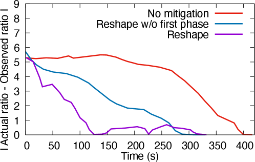
We evaluated the effect of skew and the different mitigation strategies on the results shown to the user. We ran the experiment on cores ( machines). California (location ) produced the highest number of tweets (M) in the tweet dataset. Arizona (location ) and Illinois (location ) produced M and M tweets, respectively. In the unmitigated case, the tuples of California (CA), Arizona (AZ), and Illinois (IL) were processed by workers , , and , respectively. We performed two sets of experiments, in which we mitigated the load on worker processing CA tweets by using different helper workers. In the first set of experiments, we used worker as the helper and monitored the ratio of CA to AZ tweets processed by the join operator. In the second set, we used worker as the helper and monitored the ratio of CA to IL tweets processed by the join operator. The line charts in Figure 16 and 17 show the absolute difference of the observed ratio from the actual ratio as execution progressed. In the tweet dataset, the actual ratio of CA to AZ tweets was and CA to IL tweets was .


No mitigation: When there was no mitigation, the CA, AZ, and IL tweets were processed at a similar rate as explained in Section 3.1. The observed ratio remained close to till worker was about to finish processing AZ tweets in Figure 16 and worker was about to finish IL tweets in Figure 17. The observed ratio started to increase (absolute difference of observed ratio with actual ratio started to decrease) after that because worker continued to process CA tweets. The actual ratio was observed near the end of execution (about seconds) in the unmitigated case.
Flux: It used the SBK load-transfer approach. It had the limitation of not being able to split the processing of a single key over multiple workers. The skewed worker , apart from CA, was also processing the tweets from West Virginia. The processing of the tweets from West Virginia (about K) was moved to the helper worker by Flux. However, this did affect the observed ratio of tweets much.
Flow-Join: It used the SBR approach. The execution finished earlier because the approach mitigated the skew in worker . Flow-Join had two drawbacks. First, it did not perform mitigation iteratively. It changed its partitioning logic only once based on the heavy hitters detected initially. Second, it did not consider the loads on the helper and the skewed worker while deciding the portion of the skewed worker’s load to be transferred to the helper. It always transferred % of the load of the skewed worker to the helper. The observed ratio of tweets started increasing once skew mitigation started. It reached the actual ratio seconds in Figure 16 and around seconds in Figure 17. Due to the aforementioned drawbacks, the observed ratio of tweets continued to increase even after reaching the actual ratio because the skewed worker continued to transfer 50% of its load to the helper. The observed ratio continued to increase till it reached about in Figure 16 (absolute difference = ) and in Figure 17 (absolute difference = ). At this point, the execution was near its end and the ratio started to decrease to the actual final ratio.
Reshape: It used the SBR approach and could split the processing of the CA key with a helper worker. Reshape had the advantage of iteratively adapting its partitioning logic and considered the current loads on the helper and the skewed worker while deciding the portion of load to be transferred in the second phase (Section 3.2). Thus, Reshape kept the workload of the skewed worker and the helper at similar levels. In Figure 16 and 17, after the observed ratio reaches the actual ratio at about seconds and seconds, respectively, Reshape kept the observed ratio near the actual ratio.
7.3. Benefits of the first phase
We evaluated the benefits of the first phase in Reshape as discussed in Section 3.2. We followed a similar setting as in the experiment in Section 7.2 to monitor the ratio of processed tweets. There were two mitigation strategies used in this experiment. The first one was normal Reshape, with the two phases of load transfer. In the second strategy, we disabled the first phase in Reshape and just did load transfer using the second phase. The results are plotted in Figure 18 and 19.

The first phase quickly removed the existing imbalance of load between the skewed and the helper worker when skew was detected. When the first phase was present, Reshape reached the actual ratio around and seconds in Figures 18 and 19, respectively. When the first phase was disabled, Reshape reached the actual ratio around and seconds in Figures 18 and 19, respectively. Thus, the first phase allowed Reshape to show representative results earlier. Both strategies showed more representative results than the unmitigated case.
7.4. Effect of heavy-hitter keys
California (location ) produced the highest number of tweets (M) and was a heavy-hitter key in the tweet dataset. We present the results for the mitigation of the skewed worker that processed the California key.
Load balancing ratio. The load balancing ratio at a moment during the execution is calculated by obtaining the total counts of tuples allotted to the skewed worker and its helper till that moment, and dividing the smaller value by the larger value. We periodically recorded multiple load balancing ratios during an execution and calculated their average to get the average load balancing ratio for an execution. A higher ratio is better because it represents a more balanced workload between the skewed worker and its helper.
The average load balancing ratio for the skewed worker that processed the California key and its helpers is plotted in Figure 20. A higher ratio is better because it represents a more balanced workload between the skewed worker and its helper worker. We ran the experiments on three settings by varying the number of cores up to (on machines), which was the total number of distinct locations.

Flux: It had the limitation of not being able to split the processing of a single key over multiple workers. Thus, the skewed worker processed the entire California input. The skewed worker was also processing another key with only a few hundred thousand tuples, which was moved to the helper when skew was detected. Flux had a low average load balancing ratio of about .
Flow-Join: Its main drawback was the inability to do mitigation iteratively. It changed its partitioning logic once based on the heavy-hitters detected initially. The longer it spent to detect heavy-hitters with a higher confidence, the less was the amount of future tuples left to be mitigated for finite datasets. We varied the initial duration used by Flow-Join to detect heavy-hitters from seconds to seconds. When the initial time spent was seconds, the average load balancing ratio was about and the final counts of tuples processed by the skewed and helper workers were approximately M and M, respectively. On the other hand, when the duration was seconds, the ratio was about and the final counts were approximately M and M, respectively. Flow-Join was able to reduce the execution time of on cores from seconds to seconds, when the initial detection duration was seconds.
Reshape: It split the processing of the California key with a helper worker. Reshape had the advantage of iteratively changing its partitioning logic according to input distribution using fast control messages. Thus, the skewed and helper workers ended up processing almost similar amounts of data and the average load balancing ratio was about . The execution time was reduced by 27%. In particular, Reshape was able to reduce the execution time from seconds to seconds, by mitigating the skew in running on cores.
7.5. Effect of latency of control messages
To evaluate the effect of the latency of control messages on skew handling by Reshape, we purposely added a delay between the time a worker receives a control message and the time it processes the message. Figure 21 shows the result of varying the simulated delay from second (i.e., the message is processed immediately) to seconds on the mitigation of on cores. The figure shows the average load balancing ratio for the two pairs of skewed and helper workers processing the locations of California (location ) and Texas (location ), which had the highest counts of tweets.


Impact on responsiveness of mitigation: As the control message delivery became slower, the delay between the controller sending a message and the resulting change in partitioning logic increased. Consider the example where the controller detected a workload difference of between the skewed worker and the helper worker and sent a message to start the first phase. In the case of no delay in control message delivery, the helper worker reached a similar workload as the skewed worker within seconds. In case of a delayed delivery, the workload difference continued to increase and got larger than before the first phase was started. For example, when there was a -second delay, the workload difference was at after seconds of sending the message.
Impact on load balancing. The latency in control messages affected the load sharing between skewed and helper workers. In the case of no delay, the two workers had almost similar loads and the average load balancing ratio was about as shown in Figures 21(a) and 21(b). As the delay increased, the framework was slow to react to the skew between workers, which resulted in imbalanced load-sharing. In the case of a -second delay, the average load balancing ratio reduced to about . Thus, low-latency control messages facilitated load balancing between a skewed worker and its helper.
7.6. Benefit of dynamically adjusting
We evaluated the effect of the dynamic adjustment of on skew mitigation in by Reshape on cores. We chose different values of ranging from to , and did experiments for two settings. In the first setting, was fixed for the entire execution. In the second setting, was dynamically adjusted during the execution. The mean model estimated the workload of a worker as its expected number of tuples in the next tuples and the preferred range of standard error (Section 4.3.2) was set to to tuples. We allowed up to three adjustments during an execution. Whenever had to be increased, it was increased by a fixed value of . We calculated the average load balancing ratios for the workers processing the California and Texas keys and divided them by the total number of mitigation iterations during the execution. This resulted in the metric of average load balancing per iteration, shown in Figure 22. A higher value of this metric is better because it represents a more balanced workload of skewed and helper workers in fewer iterations.

Let us first consider the cases where was dynamically adjusted to an increased value. Setting to a small value of resulted in a large number of iterations, i.e, , in the fixed setting. In the dynamic setting, the controller observed that the standard error at the beginning of the second phase was greater than and increased . Consequently, the number of iterations decreased to , which resulted in a substantial increase in the metric of average load balancing per iteration. For the cases of and in the fixed setting, the average load balancing per iteration increased with because the number of iterations decreased. The dynamic setting slightly decreased the iteration count in these cases.
Now let us consider the case where remained unchanged or decreased as a result of dynamic adjustment. When , the standard error was in the range . Thus, the dynamic adjustment did not change . When in the fixed setting, the mitigation started late and the workload of skewed and helper workers were not balanced. The mitigation was delayed even more for and in the fixed setting and the mitigation did not happen for . In the dynamic setting for the cases of , , , and , the controller observed that the standard error went below when the workload difference was about . Thus, the controller reduced to . The advantage of dynamically reducing was that it automatically started mitigation at an appropriate , even if the initial was very high.
7.7. Effect of different levels of skew
We evaluated the load balancing achieved by Reshape for different levels of skew. We used for this purpose. The data distributions in Figures 15(d)-15(e) show that the join on item_id was highly skewed and the join on date_id was moderately skewed. We evaluated the load balancing achieved for these two join operators. We scaled the data size from GB to GB. Meanwhile, we scaled the number of cores from to and did the experiments in each configuration.

Figure 23 shows the candlestick charts of the average load balancing ratios for the top five skewed workers from each of the two joins. For the highly skewed join on item_id, the skew was detected early, and there was enough time to transfer the load of the skewed workers to the helper workers. The and percentiles of the average load balancing ratios remained above for all the configurations. The median of the ratios was more than . This result shows that Reshape was able to mitigate the skew and maintain comparable workloads on the skewed and helper workers when both the input and processing power were scaled up. The join on date_id had only a moderate skew, which resulted in a delayed detection of a few of its skewed workers. Due to the delayed detection, there were fewer future tuples of skewed workers to be transferred to the helpers. Thus the ratios for the join on date_id were lower than that for the join on item_id. The performance of Reshape was also shown by the reduction in the execution time. Specifically, in the case of cores, the mitigation reduced the execution time of from seconds to seconds. In the case of cores, the mitigation reduced the time from seconds to seconds.
7.8. Effect of changes in input distribution
We evaluated how load sharing was affected when the input distribution changed during the execution. We used the synthetic dataset and workflow running on cores. Both tables in the dataset had keys. The first table contained tuples uniformally distributed across the keys. The second table contained M tuples and was produced by the source operator at runtime. We fixed worker and worker as the skewed and helper worker, respectively. We altered the load on key and , which were processed by worker and respectively. Specifically, for the first M tuples, % was allotted to the key and the rest % was uniformally distributed among the remaining keys. For the next M tuples, % was allotted to the key , % to key , and the rest was uniformally distributed. Figure 24 shows the ratio of the workloads of the helper worker to the skewed worker as time progressed. We used to clearly show the effects of changing distributions.

Flux. The skewed worker was processing keys and . Flux had the limitation of not being able to split the processing of a single key over multiple workers. Upon detecting skew, Flux can only move the key with smaller load (key ) to the helper. Thus, the workload ratio of helper to skewed worker remained close to .
Flow-Join: We used a -second initial duration to detect the overloaded keys. Flow-Join identified key as overloaded and started to transfer half of its future tuples to the helper. Thus, the workload of the helper began to rise. At seconds (point X), the input distribution changed. Since Flow-Join cannot do mitigation iteratively, half of the tuples of key continued to be sent to the helper. The helper worker started receiving % () and the skewed worker started receiving % () of the input. Thus, the load on the helper rose and became more than the skewed worker.
Reshape: It started the first phase to let the helper worker quickly catch up with the skewed worker. Thus, the load of the helper sharply increased initially. After that the second phase started and the workload ratio got closer to . At seconds (point B), the input distribution changed. At point (point C), Reshape started another iteration of mitigation and adjusted the partitioning logic according to the new input distribution. As a result, the ratio of the workloads of the workers remained close to .
7.9. Metric-collection overhead
We evaluated the metric-collection overhead of Reshape on the workflow . We scaled the data size from GB to GB. Meanwhile, we scaled the number of cores from (on machines) to (on machines) and did the experiments in each configuration. We disabled skew mitigation and executed with and without metric collection to record the metric-collection overhead. As shown in Figure 25, the overhead was around -% for all the configurations.

7.10. Performance of Reshape on sort
To evaluate its generality to other operators, we implemented Reshape for the sort operator. We used the workflow for this experiment. The Orders table was range-partitioned on its totalPrice attribute. Table 2 lists the various percentile values of the average load balancing ratio for the skewed workers that received more than M tuples in the unmitigated case (Figure 15(b)). We scaled the data size and number of cores simultaneously from GB on cores to GB on cores, and did the experiment in each configuration.
| # workers | |||||
| 20 | 0.90 | 0.92 | 0.93 | 0.935 | 0.95 |
| 40 | 0.84 | 0.87 | 0.89 | 0.90 | 0.91 |
| 60 | 0.83 | 0.85 | 0.90 | 0.91 | 0.92 |
| 80 | 0.83 | 0.84 | 0.86 | 0.87 | 0.90 |
As the number of cores increased, the and percentiles of the average load balancing ratios remained close to . This result shows that the skewed and helper workers had balanced workloads when both the input and processing power were scaled up. The consistent performance of Reshape was also shown by about % reduction in the execution time. Specifically, in the case of cores, the time reduced from seconds to seconds. In the case of cores, the time reduced from seconds to seconds.
7.11. Effect of multiple helper workers
We evaluated the load reduction achieved when multiple helper workers are assigned to a skewed worker. The experiment was done on running on cores. The most skewed worker among the workers received about M tuples in the unmitigated case. We allotted different numbers of helpers to the skewed worker and calculated the load reduction. We set the build hash-table in each worker to have keys, so that the state size became significant and the state-migration time was noticeable.

The results are plotted in Figure 26. When a single helper was used, the state migration happened in seconds. The skewed worker transferred about half of its total workload to the helper, resulting in a load reduction of M tuples. When helpers were used, the skewed worker transferred about two thirds of its tuples to the two helpers (about M each). With more helpers, the state-migration time also increased. For helpers, the state-migration time was about seconds. Thus, there were fewer future tuples left, which resulted in a small increase in the load reduction. For helpers, the state-migration time became seconds and the load reduction decreased to M. For helpers, the state-migration time was seconds and the load reduction decreased to M.
7.12. Performance of Reshape on Flink
We implemented Reshape on Apache Flink and executed on , , and cores. A worker was classified as skewed if its busyTimeMsPerSecond metric was greater than %. Figure 27 shows the average load balancing ratio for the workers processing the California and Texas tweets. The ratio was about , which means that the skewed and helper workers had similar workloads throughout the execution. For the -core case, the final counts of tuples processed by the skewed and helper workers for California were M and M, respectively. The final counts of tuples processed by the two workers for Texas on cores were M each. The execution time decreased as a result of the mitigation. For example, for the -core case, the execution time decreased from seconds to seconds.


8. Conclusions
In this paper we presented a framework called Reshape that adaptively handles partitioning skew in the exploratory data analysis setting. We presented different approaches for load transfer and analyzed their impact on the results shown to the user. We presented an analysis about the effect of the skew-detection threshold on mitigation and used it to adaptively adjust the threshold. We generalized Reshape to multiple operators and broader execution settings. We implemented Reshape on top of two big data engines and presented the results of an experimental evaluation.
References
- (1)
- Clo (2018) Cloudberry - Big Data Visualization. http://cloudberry.ics.uci.edu/.
- Abdelhamid et al. (2020) Ahmed S. Abdelhamid, Ahmed R. Mahmood, Anas Daghistani, and Walid G. Aref. 2020. Prompt: Dynamic Data-Partitioning for Distributed Micro-batch Stream Processing Systems. In Proceedings of the 2020 International Conference on Management of Data, SIGMOD Conference 2020, online conference [Portland, OR, USA], June 14-19, 2020, David Maier, Rachel Pottinger, AnHai Doan, Wang-Chiew Tan, Abdussalam Alawini, and Hung Q. Ngo (Eds.). ACM, 2455–2469. https://doi.org/10.1145/3318464.3389713
- Alteryx ([n.d.]) Alteryx Website, https://www.alteryx.com/.
- APACHE Flink ([n.d.]) Apache Flink http://flink.apache.org.
- Apache Hadoop MapReduce ([n.d.]) Apache Hadoop MapReduce, https://hadoop.apache.org/docs/stable/hadoop-mapreduce-client/hadoop-mapreduce-client-core/MapReduceTutorial.html.
- apache-samza ([n.d.]) Apache Samza. http://samza.apache.org/.
- APACHE Spark ([n.d.]) Apache Spark http://spark.apache.org.
- ApacheStorm ([n.d.]) Apache Storm, http://storm.apache.org/.
- Armbrust et al. (2018) Michael Armbrust, Tathagata Das, Joseph Torres, Burak Yavuz, Shixiong Zhu, Reynold Xin, Ali Ghodsi, Ion Stoica, and Matei Zaharia. 2018. Structured Streaming: A Declarative API for Real-Time Applications in Apache Spark. In Proceedings of the 2018 International Conference on Management of Data, SIGMOD Conference 2018, Houston, TX, USA, June 10-15, 2018, Gautam Das, Christopher M. Jermaine, and Philip A. Bernstein (Eds.). ACM, 601–613. https://doi.org/10.1145/3183713.3190664
- Auer et al. (2002) Peter Auer, Nicolò Cesa-Bianchi, and Paul Fischer. 2002. Finite-time Analysis of the Multiarmed Bandit Problem. Mach. Learn. 47, 2-3 (2002), 235–256. https://doi.org/10.1023/A:1013689704352
- Backpressure ([n.d.]) Handling Backpressure https://medium.com/@jayphelps/backpressure-explained-the-flow-of-data-through-software-2350b3e77ce7.
- Begoli et al. (2021) Edmon Begoli, Tyler Akidau, Slava Chernyak, Fabian Hueske, Kathryn Knight, Kenneth Knowles, Daniel Mills, and Dan Sotolongo. 2021. Watermarks in Stream Processing Systems: Semantics and Comparative Analysis of Apache Flink and Google Cloud Dataflow. Proc. VLDB Endow. 14, 12 (2021), 3135–3147. http://www.vldb.org/pvldb/vol14/p3135-begoli.pdf
- Beitzel et al. (2004) Steven M. Beitzel, Eric C. Jensen, Abdur Chowdhury, David A. Grossman, and Ophir Frieder. 2004. Hourly analysis of a very large topically categorized web query log. In SIGIR 2004: Proceedings of the 27th Annual International ACM SIGIR Conference on Research and Development in Information Retrieval, Sheffield, UK, July 25-29, 2004, Mark Sanderson, Kalervo Järvelin, James Allan, and Peter Bruza (Eds.). ACM, 321–328. https://doi.org/10.1145/1008992.1009048
- Benoit et al. (2013) Anne Benoit, Ümit V. Çatalyürek, Yves Robert, and Erik Saule. 2013. A survey of pipelined workflow scheduling: Models and algorithms. ACM Comput. Surv. 45, 4 (2013), 50:1–50:36. https://doi.org/10.1145/2501654.2501664
- Bindschaedler et al. (2018) Laurent Bindschaedler, Jasmina Malicevic, Nicolas Schiper, Ashvin Goel, and Willy Zwaenepoel. 2018. Rock you like a hurricane: taming skew in large scale analytics. In Proceedings of the Thirteenth EuroSys Conference, EuroSys 2018, Porto, Portugal, April 23-26, 2018, Rui Oliveira, Pascal Felber, and Y. Charlie Hu (Eds.). ACM, 20:1–20:15. https://doi.org/10.1145/3190508.3190532
- Carbone et al. (2017) Paris Carbone, Stephan Ewen, Gyula Fóra, Seif Haridi, Stefan Richter, and Kostas Tzoumas. 2017. State Management in Apache Flink®: Consistent Stateful Distributed Stream Processing. Proc. VLDB Endow. 10, 12 (2017), 1718–1729. https://doi.org/10.14778/3137765.3137777
- Carbone et al. (2015) Paris Carbone, Gyula Fóra, Stephan Ewen, Seif Haridi, and Kostas Tzoumas. 2015. Lightweight Asynchronous Snapshots for Distributed Dataflows. CoRR abs/1506.08603 (2015). arXiv:1506.08603 http://arxiv.org/abs/1506.08603
- Chaudhuri et al. (1998) Surajit Chaudhuri, Rajeev Motwani, and Vivek R. Narasayya. 1998. Random Sampling for Histogram Construction: How much is enough?. In SIGMOD 1998, Proceedings ACM SIGMOD International Conference on Management of Data, June 2-4, 1998, Seattle, Washington, USA, Laura M. Haas and Ashutosh Tiwary (Eds.). ACM Press, 436–447. https://doi.org/10.1145/276304.276343
- Chen et al. (2015) Qi Chen, Jinyu Yao, and Zhen Xiao. 2015. LIBRA: Lightweight Data Skew Mitigation in MapReduce. IEEE Trans. Parallel Distributed Syst. 26, 9 (2015), 2520–2533. https://doi.org/10.1109/TPDS.2014.2350972
- DeWitt et al. (1992) David J. DeWitt, Jeffrey F. Naughton, Donovan A. Schneider, and S. Seshadri. 1992. Practical Skew Handling in Parallel Joins. In 18th International Conference on Very Large Data Bases, August 23-27, 1992, Vancouver, Canada, Proceedings, Li-Yan Yuan (Ed.). Morgan Kaufmann, 27–40. http://www.vldb.org/conf/1992/P027.PDF
- Di et al. (2012) Sheng Di, Derrick Kondo, and Walfredo Cirne. 2012. Host load prediction in a Google compute cloud with a Bayesian model. In SC Conference on High Performance Computing Networking, Storage and Analysis, SC ’12, Salt Lake City, UT, USA - November 11 - 15, 2012, Jeffrey K. Hollingsworth (Ed.). IEEE/ACM, 21. https://doi.org/10.1109/SC.2012.68
- Ding et al. (2021) Bailu Ding, Surajit Chaudhuri, Johannes Gehrke, and Vivek R. Narasayya. 2021. DSB: A Decision Support Benchmark for Workload-Driven and Traditional Database Systems. Proc. VLDB Endow. 14, 13 (2021), 3376–3388. http://www.vldb.org/pvldb/vol14/p3376-ding.pdf
- Ding et al. (2015) Jianbing Ding, Tom Z. J. Fu, Richard T. B. Ma, Marianne Winslett, Yin Yang, Zhenjie Zhang, and Hongyang Chao. 2015. Optimal Operator State Migration for Elastic Data Stream Processing. CoRR abs/1501.03619 (2015). arXiv:1501.03619 http://arxiv.org/abs/1501.03619
- Einblick ([n.d.]) Einblick, https://www.einblick.ai.
- Elseidy et al. (2014) Mohammed Elseidy, Abdallah Elguindy, Aleksandar Vitorovic, and Christoph Koch. 2014. Scalable and Adaptive Online Joins. Proc. VLDB Endow. 7, 6 (2014), 441–452. https://doi.org/10.14778/2732279.2732281
- Fernandez et al. (2013) Raul Castro Fernandez, Matteo Migliavacca, Evangelia Kalyvianaki, and Peter R. Pietzuch. 2013. Integrating scale out and fault tolerance in stream processing using operator state management. In Proceedings of the ACM SIGMOD International Conference on Management of Data, SIGMOD 2013, New York, NY, USA, June 22-27, 2013, Kenneth A. Ross, Divesh Srivastava, and Dimitris Papadias (Eds.). ACM, 725–736. https://doi.org/10.1145/2463676.2465282
- Fisher et al. (2012) Danyel Fisher, Robert DeLine, Mary Czerwinski, and Steven M. Drucker. 2012. Interactions with big data analytics. Interactions 19, 3 (2012), 50–59. https://doi.org/10.1145/2168931.2168943
- Garraghan et al. (2015) Peter Garraghan, Xue Ouyang, Paul Townend, and Jie Xu. 2015. Timely Long Tail Identification through Agent Based Monitoring and Analytics. In IEEE 18th International Symposium on Real-Time Distributed Computing, ISORC 2015, Auckland, New Zealand, 13-17 April, 2015. IEEE Computer Society, 19–26. https://doi.org/10.1109/ISORC.2015.39
- Gufler et al. (2012) Benjamin Gufler, Nikolaus Augsten, Angelika Reiser, and Alfons Kemper. 2012. Load Balancing in MapReduce Based on Scalable Cardinality Estimates. In IEEE 28th International Conference on Data Engineering (ICDE 2012), Washington, DC, USA (Arlington, Virginia), 1-5 April, 2012, Anastasios Kementsietsidis and Marcos Antonio Vaz Salles (Eds.). IEEE Computer Society, 522–533. https://doi.org/10.1109/ICDE.2012.58
- Gupta et al. (2008) Chetan Gupta, Abhay Mehta, and Umeshwar Dayal. 2008. PQR: Predicting Query Execution Times for Autonomous Workload Management. In 2008 International Conference on Autonomic Computing, ICAC 2008, June 2-6, 2008, Chicago, Illinois, USA, John Strassner, Simon A. Dobson, José A. B. Fortes, and Kumar K. Goswami (Eds.). IEEE Computer Society, 13–22. https://doi.org/10.1109/ICAC.2008.12
- Hoffmann et al. (2019) Moritz Hoffmann, Andrea Lattuada, Frank McSherry, Vasiliki Kalavri, John Liagouris, and Timothy Roscoe. 2019. Megaphone: Latency-conscious state migration for distributed streaming dataflows. Proc. VLDB Endow. 12, 9 (2019), 1002–1015. https://doi.org/10.14778/3329772.3329777
- Hsieh et al. (2018) Kevin Hsieh, Ganesh Ananthanarayanan, Peter Bodík, Shivaram Venkataraman, Paramvir Bahl, Matthai Philipose, Phillip B. Gibbons, and Onur Mutlu. 2018. Focus: Querying Large Video Datasets with Low Latency and Low Cost. In 13th USENIX Symposium on Operating Systems Design and Implementation, OSDI 2018, Carlsbad, CA, USA, October 8-10, 2018, Andrea C. Arpaci-Dusseau and Geoff Voelker (Eds.). USENIX Association, 269–286. https://www.usenix.org/conference/osdi18/presentation/hsieh
- Kim et al. (2016) In Kee Kim, Wei Wang, Yanjun Qi, and Marty Humphrey. 2016. Empirical Evaluation of Workload Forecasting Techniques for Predictive Cloud Resource Scaling. In 9th IEEE International Conference on Cloud Computing, CLOUD 2016, San Francisco, CA, USA, June 27 - July 2, 2016. IEEE Computer Society, 1–10. https://doi.org/10.1109/CLOUD.2016.0011
- Knime ([n.d.]) Knime Website, https://www.knime.com/.
- Kulkarni et al. (2011) Anagha Kulkarni, Jaime Teevan, Krysta M. Svore, and Susan T. Dumais. 2011. Understanding temporal query dynamics. In Proceedings of the Forth International Conference on Web Search and Web Data Mining, WSDM 2011, Hong Kong, China, February 9-12, 2011, Irwin King, Wolfgang Nejdl, and Hang Li (Eds.). ACM, 167–176. https://doi.org/10.1145/1935826.1935862
- Kumar et al. (2020) Avinash Kumar, Zuozhi Wang, Shengquan Ni, and Chen Li. 2020. Amber: A Debuggable Dataflow System Based on the Actor Model. Proc. VLDB Endow. 13, 5 (2020), 740–753. https://doi.org/10.14778/3377369.3377381
- Kwon et al. (2012) YongChul Kwon, Magdalena Balazinska, Bill Howe, and Jerome A. Rolia. 2012. SkewTune: mitigating skew in mapreduce applications. In Proceedings of the ACM SIGMOD International Conference on Management of Data, SIGMOD 2012, Scottsdale, AZ, USA, May 20-24, 2012, K. Selçuk Candan, Yi Chen, Richard T. Snodgrass, Luis Gravano, and Ariel Fuxman (Eds.). ACM, 25–36. https://doi.org/10.1145/2213836.2213840
- Mai et al. (2018) Luo Mai, Kai Zeng, Rahul Potharaju, Le Xu, Steve Suh, Shivaram Venkataraman, Paolo Costa, Terry Kim, Saravanam Muthukrishnan, Vamsi Kuppa, Sudheer Dhulipalla, and Sriram Rao. 2018. Chi: A Scalable and Programmable Control Plane for Distributed Stream Processing Systems. Proc. VLDB Endow. 11, 10 (2018), 1303–1316. https://doi.org/10.14778/3231751.3231765
- Metwally et al. (2005) Ahmed Metwally, Divyakant Agrawal, and Amr El Abbadi. 2005. Efficient Computation of Frequent and Top-k Elements in Data Streams. In Database Theory - ICDT 2005, 10th International Conference, Edinburgh, UK, January 5-7, 2005, Proceedings (Lecture Notes in Computer Science), Thomas Eiter and Leonid Libkin (Eds.), Vol. 3363. Springer, 398–412. https://doi.org/10.1007/978-3-540-30570-5_27
- Monte et al. (2020) Bonaventura Del Monte, Steffen Zeuch, Tilmann Rabl, and Volker Markl. 2020. Rhino: Efficient Management of Very Large Distributed State for Stream Processing Engines. In Proceedings of the 2020 International Conference on Management of Data, SIGMOD Conference 2020, online conference [Portland, OR, USA], June 14-19, 2020, David Maier, Rachel Pottinger, AnHai Doan, Wang-Chiew Tan, Abdussalam Alawini, and Hung Q. Ngo (Eds.). ACM, 2471–2486. https://doi.org/10.1145/3318464.3389723
- Nasir et al. (2015) Muhammad Anis Uddin Nasir, Gianmarco De Francisci Morales, David García-Soriano, Nicolas Kourtellis, and Marco Serafini. 2015. The power of both choices: Practical load balancing for distributed stream processing engines. In 31st IEEE International Conference on Data Engineering, ICDE 2015, Seoul, South Korea, April 13-17, 2015, Johannes Gehrke, Wolfgang Lehner, Kyuseok Shim, Sang Kyun Cha, and Guy M. Lohman (Eds.). IEEE Computer Society, 137–148. https://doi.org/10.1109/ICDE.2015.7113279
- Nasir et al. (2016) Muhammad Anis Uddin Nasir, Gianmarco De Francisci Morales, Nicolas Kourtellis, and Marco Serafini. 2016. When two choices are not enough: Balancing at scale in Distributed Stream Processing. In 32nd IEEE International Conference on Data Engineering, ICDE 2016, Helsinki, Finland, May 16-20, 2016. IEEE Computer Society, 589–600. https://doi.org/10.1109/ICDE.2016.7498273
- Popescu et al. (2012) Adrian Daniel Popescu, Vuk Ercegovac, Andrey Balmin, Miguel Branco, and Anastasia Ailamaki. 2012. Same Queries, Different Data: Can We Predict Runtime Performance?. In Workshops Proceedings of the IEEE 28th International Conference on Data Engineering, ICDE 2012, Arlington, VA, USA, April 1-5, 2012, Anastasios Kementsietsidis and Marcos Antonio Vaz Salles (Eds.). IEEE Computer Society, 275–280. https://doi.org/10.1109/ICDEW.2012.66
- Prediction interval ([n.d.]) Prediction interval, https://otexts.com/fpp2/prediction-intervals.html.
- Ramakrishnan et al. (2012) Smriti R. Ramakrishnan, Garret Swart, and Aleksey Urmanov. 2012. Balancing reducer skew in MapReduce workloads using progressive sampling. In ACM Symposium on Cloud Computing, SOCC ’12, San Jose, CA, USA, October 14-17, 2012, Michael J. Carey and Steven Hand (Eds.). ACM, 16. https://doi.org/10.1145/2391229.2391245
- RapidMiner ([n.d.]) RapidMiner Website, https://rapidminer.com/.
- Rödiger et al. (2016) Wolf Rödiger, Sam Idicula, Alfons Kemper, and Thomas Neumann. 2016. Flow-Join: Adaptive skew handling for distributed joins over high-speed networks. In 32nd IEEE International Conference on Data Engineering, ICDE 2016, Helsinki, Finland, May 16-20, 2016. IEEE Computer Society, 1194–1205. https://doi.org/10.1109/ICDE.2016.7498324
- Shah et al. (2003) Mehul A. Shah, Joseph M. Hellerstein, Sirish Chandrasekaran, and Michael J. Franklin. 2003. Flux: An Adaptive Partitioning Operator for Continuous Query Systems. In Proceedings of the 19th International Conference on Data Engineering, March 5-8, 2003, Bangalore, India, Umeshwar Dayal, Krithi Ramamritham, and T. M. Vijayaraman (Eds.). IEEE Computer Society, 25–36. https://doi.org/10.1109/ICDE.2003.1260779
- Shen et al. (2011) Zhiming Shen, Sethuraman Subbiah, Xiaohui Gu, and John Wilkes. 2011. CloudScale: elastic resource scaling for multi-tenant cloud systems. In ACM Symposium on Cloud Computing in conjunction with SOSP 2011, SOCC ’11, Cascais, Portugal, October 26-28, 2011, Jeffrey S. Chase and Amr El Abbadi (Eds.). ACM, 5. https://doi.org/10.1145/2038916.2038921
- sparkaqewebsite ([n.d.]) Adaptive Query Execution in Spark. https://spark.apache.org/docs/latest/sql-performance-tuning.html#adaptive-query-execution.
- Statistical forecasting ([n.d.]) Statistical forecasting, https://people.duke.edu/~rnau/411home.htm.
- tpch ([n.d.]) TPC-H Website, http://www.tpc.org/tpch/.
- Vartak et al. ([n.d.]) Manasi Vartak, Harihar Subramanyam, Wei-En Lee, Srinidhi Viswanathan, Saadiyah Husnoo, Samuel Madden, and Matei Zaharia. [n.d.]. ModelDB: a system for machine learning model management. In HILDA@SIGMOD’16.
- Vitorovic et al. (2016) Aleksandar Vitorovic, Mohammed Elseidy, and Christoph Koch. 2016. Load balancing and skew resilience for parallel joins. In 32nd IEEE International Conference on Data Engineering, ICDE 2016, Helsinki, Finland, May 16-20, 2016. IEEE Computer Society, 313–324. https://doi.org/10.1109/ICDE.2016.7498250
- Wang et al. (2020) Zuozhi Wang, Avinash Kumar, Shengquan Ni, and Chen Li. 2020. Demonstration of Interactive Runtime Debugging of Distributed Dataflows in Texera. Proc. VLDB Endow. 13, 12 (2020), 2953–2956. http://www.vldb.org/pvldb/vol13/p2953-wang.pdf
- Xiao et al. (2013) Zhen Xiao, Weijia Song, and Qi Chen. 2013. Dynamic Resource Allocation Using Virtual Machines for Cloud Computing Environment. IEEE Trans. Parallel Distributed Syst. 24, 6 (2013), 1107–1117. https://doi.org/10.1109/TPDS.2012.283
- Xu et al. (2022) Zhuangdi Xu, Gaurav Tarlok Kakkar, Joy Arulraj, and Umakishore Ramachandran. 2022. EVA: A Symbolic Approach to Accelerating Exploratory Video Analytics with Materialized Views. In SIGMOD ’22: International Conference on Management of Data, Philadelphia, PA, USA, June 12 - 17, 2022, Zachary Ives, Angela Bonifati, and Amr El Abbadi (Eds.). ACM, 602–616. https://doi.org/10.1145/3514221.3526142
- Yan et al. (2013) Wei Yan, Yuan Xue, and Bradley A. Malin. 2013. Scalable and robust key group size estimation for reducer load balancing in MapReduce. In Proceedings of the 2013 IEEE International Conference on Big Data, 6-9 October 2013, Santa Clara, CA, USA, Xiaohua Hu, Tsau Young Lin, Vijay V. Raghavan, Benjamin W. Wah, Ricardo Baeza-Yates, Geoffrey C. Fox, Cyrus Shahabi, Matthew Smith, Qiang Yang, Rayid Ghani, Wei Fan, Ronny Lempel, and Raghunath Nambiar (Eds.). IEEE Computer Society, 156–162. https://doi.org/10.1109/BigData.2013.6691568
- Yun et al. (2020) Daqing Yun, Wuji Liu, Chase Q. Wu, Nageswara S. V. Rao, and Rajkumar Kettimuthu. 2020. Performance Prediction of Big Data Transfer Through Experimental Analysis and Machine Learning. In 2020 IFIP Networking Conference, Networking 2020, Paris, France, June 22-26, 2020. IEEE, 181–189. https://ieeexplore.ieee.org/document/9142699