This paper was converted on www.awesomepapers.org from LaTeX by an anonymous user.
Want to know more? Visit the Converter page.

Representations of a quantum-deformed Lorentz algebra, Clebsch-Gordan map, and Fenchel-Nielsen representation of quantum complex flat connections at level-𝒌\bm{k}

Muxin Han
Abstract

A family of infinite-dimensional irreducible \star-representations on L2()k\mathcal{H}\simeq L^{2}(\mathbb{R})\otimes\mathbb{C}^{k} is defined for a quantum-deformed Lorentz algebra U𝐪(sl2)U𝐪~(sl2)U_{\mathbf{q}}(sl_{2})\otimes U_{\tilde{\mathbf{q}}}(sl_{2}), where 𝐪=exp[2πik(1+b2)]\mathbf{q}=\exp[\frac{2\pi i}{k}(1+b^{2})] and 𝐪~=exp[2πik(1+b2)]\tilde{\mathbf{q}}=\exp[\frac{2\pi i}{k}(1+b^{-2})] with k+k\in\mathbb{Z}_{+} and |b|=1|b|=1. The representations are constructed with the irreducible representation of quantum torus algebra at level-kk, which is developed from the quantization of SL(2,)\mathrm{SL}(2,\mathbb{C}) Chern-Simons theory. We study the Clebsch-Gordan decomposition of the tensor product representation, and we show that it reduces to the same problem as diagonalizing the complex Fenchel-Nielson length operators in quantizing SL(2,)\mathrm{SL}(2,\mathbb{C}) flat connections on 4-holed sphere. Finally, the spectral decomposition of the complex Fenchel-Nielson length operators results in the direct-integral representation of the Hilbert space \mathcal{H}, which we call the Fenchel-Nielson representation.

1 Introduction

This work is partly inspired by the early results on the relations between the modular double of Uq(sl(2,))U_{q}(sl(2,\mathbb{R})) and quantum Teichmüeller theory [1, 2, 3, 4, 5, 6, 7]. As has been shown in the literature, the representation of the modular double of Uq(sl(2,))U_{q}(sl(2,\mathbb{R})) can be defined on L2()L^{2}(\mathbb{R}), where the representations of the generators relate to the representation of quantum torus algebra (composed by the generators of Weyl algebra). For the tensor product representation, the Clebsch-Gordan decomposition is equivalent to the spectral decomposition of certain Fenchel-Nielsen (FN) length operator in quantum Teichmüeller theory. These results find their generalizations in this paper.

The quantum Teichmüeller theory closely relates to the SL(2,)\mathrm{SL}(2,\mathbb{R}) Chern-Simons theory [8, 9]. There has been recent generalization in [10, 11, 12] to the Teichmüeller TQFT of integer level, which relates to the quantization of Chern-Simons theory with complex gauge group SL(2,)\mathrm{SL}(2,\mathbb{C}). The quantum SL(2,)\mathrm{SL}(2,\mathbb{C}) Chern-Simons theory has the complex coupling constant =2πik(1+b2),~=2πik(1+b2)\hbar=\frac{2\pi i}{k}(1+b^{2}),\ \tilde{\hbar}=\frac{2\pi i}{k}(1+b^{-2}) with k,|b|=1k\in\mathbb{Z},\ |b|=1 (for one of the unitary branch [13]). The integer kk is called the level of Chern-Simons theory and relates to the integer level of the Teichmüeller TQFT. The quantization of SL(2,)\mathrm{SL}(2,\mathbb{C}) Chern-Simons theory results in the Weyl algebra and quantum torus algebra at level-kk, motivated by quantizing the Chern-Simon symplectic structure [12, 10]. The Weyl algebra has 𝐪=exp()\mathbf{q}=\exp(\hbar) and 𝐪~=exp(~)\tilde{\mathbf{q}}=\exp(\tilde{\hbar}), and the level-kk quantum torus algebra has q=exp(/2)q=\exp(\hbar/2) and q~=exp(~/2)\tilde{q}=\exp(\tilde{\hbar}/2). The Hilbert space carrying the representation is L2()k\mathcal{H}\simeq L^{2}(\mathbb{R})\otimes\mathbb{C}^{k}, and the representation reduces to the representation in quantum Teichmüeller theory [5, 14] when k=1k=1. The representation of quantum torus algebra at level-kk is reviewed in Section 2.

Based on the representation of the quantum torus algebra, we construct a family of irreducible representation of U𝐪(sl2)U𝐪~(sl2)U_{\mathbf{q}}(sl_{2})\otimes U_{\tilde{\mathbf{q}}}(sl_{2}) on \mathcal{H}. The star-structure on U𝐪(sl2)U𝐪~(sl2)U_{\mathbf{q}}(sl_{2})\otimes U_{\tilde{\mathbf{q}}}(sl_{2}) is represented by the hermitian conjugate on \mathcal{H}. As the tensor product of two Hopf algebras, U𝐪(sl2)U𝐪~(sl2)U_{\mathbf{q}}(sl_{2})\otimes U_{\tilde{\mathbf{q}}}(sl_{2}) has a well-defined Hopf algebra structure and can be understood as a quantum deformation of the Lorentz algebra. In particular, it is a generalization of the quantum Lorentz group with real 𝐪\mathbf{q} that is well-studied in the literature (see e.g.[15, 16]). The irreducible representations are parametrized by a continuous parameter μL\mu_{L}\in\mathbb{R} and a discrete parameter mL/km_{L}\in\mathbb{Z}/k\mathbb{Z}. They may be viewed as analog with the principle-series unitary representation of SL(2,)\mathrm{SL}(2,\mathbb{C}), although they are periodic in mLm_{L}.

We study the Clebsch-Gordan decomposition of the tensor product representation (of U𝐪(sl2)U𝐪~(sl2)U_{\mathbf{q}}(sl_{2})\otimes U_{\tilde{\mathbf{q}}}(sl_{2})) on \mathcal{H}\otimes\mathcal{H}, and we show that the result is a direct-integral of irreducible representations (see Section 3.2). The direct-integral is given by the spectral decomposition of the Casimir operator Q21Q_{21} of the tensor product representation, and we find the unitary transformation 𝒰21\mathcal{U}_{21} as the Clebsch-Gordan map representing the co-multiplication.

Interestingly Q21Q_{21} relates to the quantization of complex FN lengths for SL(2,)\mathrm{SL}(2,\mathbb{C}) flat connections on 4-holed sphere (see Section 4). As resulting from quantizing the SL(2,)\mathrm{SL}(2,\mathbb{C}) Chern-Simons theory, the quantization of SL(2,)\mathrm{SL}(2,\mathbb{C}) flat connections on 4-holed sphere can be constructed based on the level-kk representation of quantum torus algebra. We focus on the case that k=2Nk=2N is even (NN is odd). In this case, we have the decomposition +\mathcal{H}\simeq\mathcal{H}_{+}\oplus\mathcal{H}_{-} where each of ±L2()N\mathcal{H}_{\pm}\simeq L^{2}(\mathbb{R})\otimes\mathbb{C}^{N} carries the irreducible representation of the quantum algebra from quantizing the Fock-Goncharov (FG) coordinates of flat connections. The complex FN length that relates to Q21Q_{21} is given by the trace of holonomies around two holes. It turns out that the quantization of the complex FN length leads to the normal operators 𝑳,𝑳~=𝑳\bm{L},\tilde{\bm{L}}=\bm{L}^{\dagger}, and id𝑳\mathrm{id}_{\mathcal{H}}\otimes\bm{L} is represented the same as Q21Q_{21} on \mathcal{H}\otimes\mathcal{H} up to a unitary transformation. Moreover, we show that the traces of S-cycle (enclosing the 1st and 2nd holes) and T-cycle (enclosing the 2nd and 3rd holes) holonomies are related by a unitary transformation, which is a realization of the A-move in the Moore-Seiberg groupoid (as a generalizaton from [6]).

We show in Section 5 that the spectral decomposition of 𝑳,𝑳~\bm{L},\tilde{\bm{L}} endows to \mathcal{H} the direct-integral representation, which we call the FN representation:

mr/k0dμrρ(μr,mr)1μr,mr,\displaystyle\mathcal{H}\simeq\sum_{m_{r}\in\mathbb{Z}/k\mathbb{Z}}\int_{0}^{\infty}\mathrm{d}\mu_{r}\rho(\mu_{r},m_{r})^{-1}\,\mathcal{H}_{\mu_{r},m_{r}}, (1.1)

where dμrρ(μr,mr)1\mathrm{d}\mu_{r}\rho(\mu_{r},m_{r})^{-1} is the spectral measure and each μr,mr\mathcal{H}_{\mu_{r},m_{r}} is 1-dimensional. The spectra of 𝑳,𝑳~\bm{L},\tilde{\bm{L}} are respectively (r)=r+r1\ell(r)=r+r^{-1} and (r)\ell(r)^{*}, where r=exp[2πik(ibμrmr)]r=\exp[\frac{2\pi i}{k}(-ib\mu_{r}-m_{r})]. Due to the relation between 𝑳\bm{L} and Q12Q_{12}, the direct-integral representation (1.1) also gives the Clebsch-Gordan decomposition for the tensor product representation of U𝐪(sl2)U𝐪~(sl2)U_{\mathbf{q}}(sl_{2})\otimes U_{\tilde{\mathbf{q}}}(sl_{2}).

The results from this work should have impact on the complex Chern-Simons theory at level-kk and its relation to quantum group and quantum Teichmüeller theory. For instance, although the quantum Lorentz group with real deformation and the representation theory has been widely studied, the generalization to complex 𝐪\mathbf{q} has not been studied in the literature before. We show in this paper that this generalization closely relates to the SL(2,)\mathrm{SL}(2,\mathbb{C}) Chern-Simons theory with level-kk 111The quantum Lorentz group with real deformation relates to the SL(2,)\mathrm{SL}(2,\mathbb{C}) Chern-Simons theory with k=0k=0 [17].. As another aspect, given the relation between quantum Teichmüeller theory and Liouville conformal field theory, our study might point toward certain generalization of Liouville conformal field theory relating to the level-k, and this generalization might also relate to the boundary field theory of the SL(2,)\mathrm{SL}(2,\mathbb{C}) Chern-Simons theory.

In addition to the above, another motivation of this work is the potential application to the spinfoam model with cosmological constant in Loop Quantum Gravity [18, 19, 20]. The spinfoam model is formulated with SL(2,)\mathrm{SL}(2,\mathbb{C}) Chern-Simons theory (1/k1/k is proportional to the absolute value of cosmological constant) with the special boundary condition called the simplicity constraint, which restricts the flat connections on 4-holed sphere to be SU(2) up to conjugation. Classically, the simplicity constraint is conveniently formulated in terms of the complex FN variables [21]. Therefore, it may be convenient to formulate the quantization of the simplicity constraint in the FN representation of quantum flat connections. The investigation on this perspective will be reported elsewhere.

The structure of this paper is as follows: In Section 2, we review briefly the representation of quantum torus algebra at level-kk and set up some notations. In section 3, we construct the representations of U𝐪(sl2)U𝐪~(sl2)U_{\mathbf{q}}(sl_{2})\otimes U_{\tilde{\mathbf{q}}}(sl_{2}) and discussion the Clebsch-Gordan decomposition of tensor product representation. In Section 4, we discuss the quantization of SL(2,)\mathrm{SL}(2,\mathbb{C}) flat connections on 4-holed sphere with a certain ideal triangulation, and we discuss the S-cycle and T-cycle trace operators and their unitary transformations. In Section 5, we compute the eigenvalue and distributional eigenstates of the trace operators and prove the direct-integral decomposition of the Hilbert space. In Section 6, we discuss the unitary transformation induced by changing ideal triangulation of the 4-holed sphere.

2 Quantum torus algebra and the representation at level-kk

The quantum torus algebra 𝒪q(𝕋2)\mathcal{O}_{q}(\mathbb{T}^{2}) is spanned by Laurent polynomials of the symbols 𝒙α,β\bm{x}_{\alpha,\beta} with α,β\alpha,\beta\in\mathbb{Z}, satisfying the following relation

𝒙α,β𝒙γ,δ=qαδβγ𝒙α+γ,β+δ,q=e/2.\bm{x}_{\alpha,\beta}\bm{x}_{\gamma,\delta}=q^{\alpha\delta-\beta\gamma}\bm{x}_{\alpha+\gamma,\beta+\delta},\qquad q=e^{\hbar/2}. (2.1)

where \hbar\in\mathbb{C} is the quantum deformation parameter. We associated to 𝒪q(𝕋2)\mathcal{O}_{q}(\mathbb{T}^{2}) the “anti-holomorphic counterpart” 𝒪q~(𝕋2)\mathcal{O}_{\tilde{q}}(\mathbb{T}^{2}) generated by 𝒙~α,β\tilde{\bm{x}}_{\alpha,\beta} with α,β\alpha,\beta\in\mathbb{Z}, satisfying

𝒙~α,β𝒙~γ,δ=q~αδβγ𝒙~α+γ,β+δ,q~=e~/2,~=,\tilde{\bm{x}}_{\alpha,\beta}\tilde{\bm{x}}_{\gamma,\delta}=\tilde{q}^{\alpha\delta-\beta\gamma}\tilde{\bm{x}}_{\alpha+\gamma,\beta+\delta},\qquad\tilde{q}=e^{\tilde{\hbar}/2},\qquad\tilde{\hbar}=-\hbar^{*}, (2.2)

and 𝒪q~(𝕋2)\mathcal{O}_{\tilde{q}}(\mathbb{T}^{2}) commutes with 𝒪q(𝕋2)\mathcal{O}_{q}(\mathbb{T}^{2}). The entire algebra is denoted by 𝒜(𝕋2)=𝒪q(𝕋2)𝒪q~(𝕋2)\mathcal{A}_{\hbar}(\mathbb{T}^{2})=\mathcal{O}_{q}(\mathbb{T}^{2})\otimes\mathcal{O}_{\tilde{q}}(\mathbb{T}^{2}). We can endow the algebra a \star-structure by

(𝒙α,β)=𝒙~α,β,(𝒙~α,β)=𝒙α,β.\star\left(\bm{x}_{\alpha,\beta}\right)=\tilde{\bm{x}}_{\alpha,\beta},\qquad\star\left(\tilde{\bm{x}}_{\alpha,\beta}\right)=\bm{x}_{\alpha,\beta}.

which interchanges the holomorphic and antiholomorphic copies.

In this paper, we use the following parametrizations of \hbar and ~\tilde{\hbar}

=2πik(1+b2),~=2πik(1+b2),\hbar=\frac{2\pi i}{k}\left(1+b^{2}\right),\qquad\tilde{\hbar}=\frac{2\pi i}{k}\left(1+b^{-2}\right),

where k,bk,b satsifies

k+,|b|=1,Re(b)>0,Im(b)>0.k\in\mathbb{Z}_{+},\qquad|b|=1,\qquad\mathrm{Re}(b)>0,\qquad\mathrm{Im}(b)>0.

As we are going to see in Section 4, kk relates to the integer level of the SL(2,)\mathrm{SL}(2,\mathbb{C}) Chern-Simons theory.

It has been proposed in [12, 11] an infinite-dimensional unitary irreducible representation of 𝒜(𝕋2)\mathcal{A}_{\hbar}(\mathbb{T}^{2}) as the quantization of complex Chern-Simons theory. The Hilbert space carrying the representation is L2()k\mathcal{H}\simeq L^{2}(\mathbb{R})\otimes\mathbb{C}^{k}, where a state is denoted by f(μ,m),f(\mu,m), μ,\mu\in\mathbb{R}, m/km\in\mathbb{Z}/k\mathbb{Z}. The following operators are defined on \mathcal{H}

𝝁f(μ,m)\displaystyle\bm{\mu}f(\mu,m) =μf(μ,m),𝝂f(μ,m)=k2πiμf(μ,m)\displaystyle=\mu f(\mu,m),\qquad\bm{\nu}f(\mu,m)=-\frac{k}{2\pi i}\frac{\partial}{\partial\mu}f(\mu,m)
e2πik𝒎f(μ,m)\displaystyle e^{\frac{2\pi i}{k}\bm{m}}f(\mu,m) =e2πikmf(μ,m),e2πik𝒏f(μ,m)=f(μ,m+1).\displaystyle=e^{\frac{2\pi i}{k}m}f(\mu,m),\qquad e^{\frac{2\pi i}{k}\bm{n}}f(\mu,m)=f(\mu,m+1).

They satisfy

[𝝁,𝝂]=k2πi,e2πik𝒏e2πik𝒎=e2πike2πik𝒎e2πik𝒏,[𝝂,e2πik𝒎]=[𝝁,e2πik𝒏]=0\displaystyle[\bm{\mu},\bm{\nu}]=\frac{k}{2\pi i},\qquad e^{\frac{2\pi i}{k}\bm{n}}e^{\frac{2\pi i}{k}\bm{m}}=e^{\frac{2\pi i}{k}}e^{\frac{2\pi i}{k}\bm{m}}e^{\frac{2\pi i}{k}\bm{n}},\qquad[\bm{\nu},e^{\frac{2\pi i}{k}\bm{m}}]=[\bm{\mu},e^{\frac{2\pi i}{k}\bm{n}}]=0 (2.3)

The representation of 𝒙,𝒚,𝒙~,𝒚~\bm{x},\bm{y},\tilde{\bm{x}},\tilde{\bm{y}} in the quantum torus algebra are represented by

𝒚\displaystyle\bm{y} =exp[2πik(ib𝝁𝒎)],\displaystyle=\exp\left[\frac{2\pi i}{k}(-ib\boldsymbol{\mu}-\bm{m})\right], 𝒚~=exp[2πik(ib1𝝁+𝒎)],\displaystyle\qquad\tilde{\bm{y}}=\exp\left[\frac{2\pi i}{k}\left(-ib^{-1}\boldsymbol{\mu}+\bm{m}\right)\right], (2.4)
𝒙\displaystyle\bm{x} =exp[2πik(ib𝝂𝒏)],\displaystyle=\exp\left[\frac{2\pi i}{k}(-ib\boldsymbol{\nu}-\bm{n})\right], 𝒙~=exp[2πik(ib1𝝂+𝒏)].\displaystyle\qquad\tilde{\bm{x}}=\exp\left[\frac{2\pi i}{k}\left(-ib^{-1}\boldsymbol{\nu}+\bm{n}\right)\right]. (2.5)

Their actions on states f(μ,m)f(\mu,m) are given by

𝒚f(μ,m)\displaystyle\bm{y}f(\mu,m) =e2πik(ibμm)f(μ,m),\displaystyle=e^{\frac{2\pi i}{k}(-ib{\mu}-{m})}f(\mu,m),\qquad 𝒙f(μ,m)=f(μ+ib,m1),\displaystyle\bm{x}f(\mu,m)=f(\mu+ib,m-1), (2.6)
𝒚~f(μ,m)\displaystyle\tilde{\bm{y}}f(\mu,m) =e2πik(ib1μ+m)f(μ,m),\displaystyle=e^{\frac{2\pi i}{k}(-ib^{-1}{\mu}+{m})}f(\mu,m),\qquad 𝒙~f(μ,m)=f(μ+ib1,m+1).\displaystyle\tilde{\bm{x}}f(\mu,m)=f(\mu+ib^{-1},m+1). (2.7)

These operators form the 𝐪,𝐪~\mathbf{q},\tilde{\mathbf{q}}-Weyl algebra with 𝐪=q2=e\mathbf{q}=q^{2}=e^{\hbar}, and 𝐪~=q~2=e~\tilde{\mathbf{q}}=\tilde{q}^{2}=e^{\tilde{\hbar}}:

𝒙𝒚=𝐪𝒚𝒙,𝒙~𝒚~=𝐪~𝒚~𝒙~,𝒙𝒚~=𝒚~𝒙,𝒙~𝒚=𝒚𝒙~.\bm{x}\bm{y}=\mathbf{q}\bm{y}\bm{x},\qquad\tilde{\bm{x}}\tilde{\bm{y}}=\tilde{\mathbf{q}}\tilde{\bm{y}}\tilde{\bm{x}},\qquad\bm{x}\tilde{\bm{y}}=\tilde{\bm{y}}\bm{x},\qquad\tilde{\bm{x}}{\bm{y}}={\bm{y}}\tilde{\bm{x}}.

The tilded and untilded operators are related by the Hermitian conjugate

𝒙=𝒙~,𝒚=𝒚~,\bm{x}^{\dagger}=\tilde{\bm{x}},\qquad\bm{y}^{\dagger}=\tilde{\bm{y}},

and they are normal operators. It is often convenient to use the following formal notation

𝒙=e𝑿,𝒚=e𝒀;𝒙~=e𝑿~,𝒚~=e𝒀~\bm{x}=e^{\bm{X}},\qquad\bm{y}=e^{\bm{Y}};\qquad\tilde{\bm{x}}=e^{\tilde{\bm{X}}},\qquad\tilde{\bm{y}}=e^{\tilde{\bm{Y}}}

where

𝒀\displaystyle\bm{Y} =2πik(ib𝝁𝒎),𝒀~=2πik(ib1𝝁+𝒎),\displaystyle=\frac{2\pi i}{k}(-ib\boldsymbol{\mu}-\bm{m}),\qquad\tilde{\bm{Y}}=\frac{2\pi i}{k}\left(-ib^{-1}\boldsymbol{\mu}+\bm{m}\right),
𝑿\displaystyle\bm{X} =2πik(ib𝝂𝒏),𝑿~=2πik(ib1𝝂+𝒏),\displaystyle=\frac{2\pi i}{k}(-ib\boldsymbol{\nu}-\bm{n}),\qquad\tilde{\bm{X}}=\frac{2\pi i}{k}\left(-ib^{-1}\boldsymbol{\nu}+\bm{n}\right),

satisfy the canonical commutation relation

[𝑿,𝒀]=,[𝑿~,𝒀~]=~,[𝑿,𝒀~]=[𝑿~,𝒀]=0.[\bm{X},\bm{Y}]=\hbar,\qquad[\tilde{\bm{X}},\tilde{\bm{Y}}]=\tilde{\hbar},\qquad[\bm{X},\tilde{\bm{Y}}]=[\tilde{\bm{X}},{\bm{Y}}]=0.

The operators 𝒙,𝒙~,𝒚,𝒚~\bm{x},\tilde{\bm{x}},\bm{y},\tilde{\bm{y}} are unbounded operators. The common domain 𝔇\mathfrak{D} of their Laurent polynomials contains f(μ,m)f(\mu,m) being entire functions in μ\mu and satisfying

eα2πkbμf(μ,m)L2(),f(μ+ibα,m)L2(),m/k,α.e^{\alpha\frac{2\pi}{k}b\mu}f(\mu,m)\in L^{2}(\mathbb{R}),\qquad f(\mu+ib\alpha,m)\in L^{2}(\mathbb{R}),\qquad\forall\,m\in\mathbb{Z}/k\mathbb{Z},\quad\alpha\in\mathbb{Z}.

The Hermite functions eμ2/2Hn(μ)e^{-\mu^{2}/2}H_{n}(\mu) , n=1,,n=1,\cdots,\infty satisfy all the requirements and span a dense domain in L2()L^{2}(\mathbb{R}), so 𝔇\mathfrak{D} is dense in \mathcal{H}.

We denote by (𝔇)\mathcal{L}(\mathfrak{D}) the space of linear operators on 𝔇\mathfrak{D}. The representation ρ\rho: 𝒜(𝕋2)(𝔇)\mathcal{A}_{\hbar}(\mathbb{T}^{2})\to\mathcal{L}(\mathfrak{D}) is given by

ρ:\displaystyle\rho:\ 𝒙α,βeα𝑿+β𝒀=qαβ𝒙α𝒚β,\displaystyle\bm{x}_{\alpha,\beta}\mapsto e^{\alpha\bm{X}+\beta\bm{Y}}=q^{-\alpha\beta}\bm{x}^{\alpha}\bm{y}^{\beta}, (2.8)
𝒙~α,βeα𝑿~+β𝒀~=q~αβ𝒙~α𝒚~β.\displaystyle\tilde{\bm{x}}_{\alpha,\beta}\mapsto e^{\alpha\tilde{\bm{X}}+\beta\tilde{\bm{Y}}}=\tilde{q}^{-\alpha\beta}\tilde{\bm{x}}^{\alpha}\tilde{\bm{y}}^{\beta}. (2.9)

The relations (2.1) and (2.2) are obtained by appyling the (𝐪,𝐪~)(\mathbf{q},\tilde{\mathbf{q}})-Weyl algebra. In the following, we often denote ρ(𝒙α,β\rho(\bm{x}_{\alpha,\beta}) by 𝒙α,β\bm{x}_{\alpha,\beta} for simplifying notations. The \star-stucture is represened by the Hermitian conjugate

𝒙α,β=q~αβ𝒚~β𝒙~α=q~αβ𝒙~α𝒚~β=𝒙~α,β.\bm{x}_{\alpha,\beta}^{\dagger}=\tilde{q}^{\alpha\beta}\tilde{\bm{y}}^{\beta}\tilde{\bm{x}}^{\alpha}=\tilde{q}^{-\alpha\beta}\tilde{\bm{x}}^{\alpha}\tilde{\bm{y}}^{\beta}=\tilde{\bm{x}}_{\alpha,\beta}.

3 Representation of a q-deformed Lorentz algebra

3.1 The representation

Based on the representation (,ρ)(\mathcal{H},\rho) of the quantum torus algebra and by the linear combinations of the operators 𝒙αβ\bm{x}_{\alpha\beta}, we obtain a representation of U𝐪(sl2)U_{{\bf q}}(sl_{2}) on \mathcal{H}. Indeed, we define a family of operators Eλ,Fλ,Kλ,Kλ1E_{\lambda},F_{\lambda},K_{\lambda},K_{\lambda}^{-1} by

Kλ\displaystyle K_{\lambda} =𝒙1,0,Kλ1=𝒙1,0,Eλ=1𝐪𝐪1𝒙1,1,\displaystyle=\bm{x}_{-1,0},\qquad K_{\lambda}^{-1}=\bm{x}_{1,0},\qquad E_{\lambda}=-\frac{1}{{\bf q}-{\bf q}^{-1}}\bm{x}_{-1,1}, (3.1)
Fλ\displaystyle F_{\lambda} =1𝐪𝐪1[(λ+λ1)𝒙1,1+𝒙3,1+𝒙1,1],\displaystyle=-\frac{1}{{\bf q}-{\bf q}^{-1}}\left[\left(\lambda+\lambda^{-1}\right)\bm{x}_{1,-1}+\bm{x}_{3,-1}+\bm{x}_{-1,-1}\right], (3.2)

where the parameter λ×\lambda\in\mathbb{C^{\times}}. It is straight-forward to check that Eλ,Fλ,Kλ,Kλ1E_{\lambda},F_{\lambda},K_{\lambda},K_{\lambda}^{-1} satisfy the commutation relation of U𝐪(sl2)U_{{\bf q}}(sl_{2}) 222See the convention in [4] up to an inverse of 𝐪\mathbf{q}.:

KλEλ=𝐪1EλKλ\displaystyle K_{\lambda}E_{\lambda}={\bf q}^{-1}E_{\lambda}K_{\lambda} ,KλFλ=𝐪FλKλ,[Eλ,Fλ]=Kλ2Kλ2𝐪𝐪1.\displaystyle,\qquad K_{\lambda}F_{\lambda}={\bf q}F_{\lambda}K_{\lambda},\qquad\left[E_{\lambda},F_{\lambda}\right]=\frac{K_{\lambda}^{2}-K_{\lambda}^{-2}}{{\bf q}-{\bf q}^{-1}}.

Similarly, we define the tilded operators

K~λ\displaystyle\tilde{K}_{\lambda} =𝒙~1,0,K~λ1=𝒙~1,0,E~λ=1𝐪~𝐪~1𝒙~1,1,\displaystyle=\tilde{\bm{x}}_{-1,0},\qquad\tilde{K}_{\lambda}^{-1}=\tilde{\bm{x}}_{1,0},\qquad\tilde{E}_{\lambda}=-\frac{1}{\tilde{{\bf q}}-\tilde{{\bf q}}^{-1}}\tilde{\bm{x}}_{-1,1},
F~λ\displaystyle\tilde{F}_{\lambda} =1𝐪~𝐪~1[(λ~+λ~1)𝒙~1,1+𝒙~3,1+𝒙~1,1],\displaystyle=-\frac{1}{\tilde{{\bf q}}-\tilde{{\bf q}}^{-1}}\left[\left(\tilde{\lambda}+\tilde{\lambda}^{-1}\right)\tilde{\bm{x}}_{1,-1}+\tilde{\bm{x}}_{3,-1}+\tilde{\bm{x}}_{-1,-1}\right],

They satisfy the commutation relation of U𝐪~(sl2)U_{\tilde{{\bf q}}}(sl_{2}):

K~λE~λ=𝐪~1E~λK~λ,K~λF~λ=𝐪~F~λK~λ\displaystyle\tilde{K}_{\lambda}\tilde{E}_{\lambda}=\tilde{{\bf q}}^{-1}\tilde{E}_{\lambda}\tilde{K}_{\lambda},\qquad\tilde{K}_{\lambda}\tilde{F}_{\lambda}=\tilde{{\bf q}}\tilde{F}_{\lambda}\tilde{K}_{\lambda} ,[E~λ,F~λ]=K~λ2K~λ2𝐪~𝐪~1.\displaystyle,\qquad\left[\tilde{E}_{\lambda},\tilde{F}_{\lambda}\right]=\frac{\tilde{K}_{\lambda}^{2}-\tilde{K}_{\lambda}^{-2}}{\tilde{{\bf q}}-\tilde{{\bf q}}^{-1}}.

It shows that \mathcal{H} carries a \star-representation of U𝐪(sl2)U𝐪~(sl2)U_{{\bf q}}(sl_{2})\otimes U_{\tilde{{\bf q}}}(sl_{2}) labelled by the parameters (λ,λ~)(\lambda,\tilde{\lambda}) with λ,λ~×\lambda,\tilde{\lambda}\in\mathbb{C^{\times}}. When λ=λ~\lambda^{*}=\tilde{\lambda}, the tilded operators and untilded operator are related by the Hermitian conjugate

K~λ=Kλ,E~λ=Eλ,F~λ=Fλ,\tilde{K}_{\lambda}=K_{\lambda}^{\dagger},\qquad\tilde{E}_{\lambda}=-E_{\lambda}^{\dagger},\qquad\tilde{F}_{\lambda}=-F_{\lambda}^{\dagger},

as the representation of the \star-structure. The minus sign is due to 𝐪=𝐪~𝟏\bf{q}^{*}=\tilde{\bf{q}}^{-1}. The representation is irreducible because the representation of the Weyl algebra is irreducible333The generators of the Weyl algebra relate to the U𝐪(sl2)U_{{\bf q}}(sl_{2}) generators by 𝒙=𝒙1,0=Kλ1\bm{x}=\bm{x}_{1,0}=K_{\lambda}^{-1}, 𝒚=𝒙0,1=q1𝒙1,0𝒙1,1=(𝐪𝐪1)q1Kλ1Eλ\bm{y}=\bm{x}_{0,1}=q^{-1}\bm{x}_{1,0}\bm{x}_{-1,1}=-(\mathbf{q}-\mathbf{q}^{-1})q^{-1}K_{\lambda}^{-1}E_{\lambda}. . We denote this representation by πλ,λ~\pi_{\lambda,\tilde{\lambda}} 444 The above representation is motivated by generalizing the representations studied in e.g. [2, 3, 1] for the modular double of Uq(SL(2,)){U}_{q}(\mathrm{SL}(2,\mathbb{R})), although here (𝐪,𝐪~)(e2πib2,e2πib2)(\mathbf{q},\tilde{\mathbf{q}})\to(e^{2\pi ib^{2}},e^{2\pi ib^{-2}}) when k=1k=1 or (𝐪,𝐪~)(eπib2(\mathbf{q},\tilde{\mathbf{q}})\to(-e^{\pi ib^{2}} and eπib2)-e^{\pi ib^{-2}}) when k=2k=2, whereas the modular deformation parameter there is q=eπib2q=e^{\pi ib^{2}} and q~=eπib2\tilde{q}=e^{\pi ib^{-2}}..

The comultiplication Δ\Delta of U𝐪(sl2)U𝐪~(sl2)U_{{\bf q}}(sl_{2})\otimes U_{\tilde{{\bf q}}}(sl_{2}) is defined by

ΔK\displaystyle\Delta K =KK,ΔE=EK+K1E,ΔF=FK+K1F,\displaystyle=K\otimes K,\qquad\Delta E=E\otimes K+K^{-1}\otimes E,\qquad\Delta F=F\otimes K+K^{-1}\otimes F,
ΔK~\displaystyle\Delta\tilde{K} =K~K~,ΔE~=E~K~+K~1E~,ΔF~=F~K~+K~1F~.\displaystyle=\tilde{K}\otimes\tilde{K},\qquad\Delta\tilde{E}=\tilde{E}\otimes\tilde{K}+\tilde{K}^{-1}\otimes\tilde{E},\qquad\Delta\tilde{F}=\tilde{F}\otimes\tilde{K}+\tilde{K}^{-1}\otimes\tilde{F}.

The Casimir operators defined by

Qλ\displaystyle Q_{\lambda} =(𝐪𝐪1)2FλEλ𝐪1Kλ2𝐪Kλ2\displaystyle=\left({\bf q}-{\bf q}^{-1}\right)^{2}F_{\lambda}E_{\lambda}-\mathbf{q}^{-1}K_{\lambda}^{2}-{\bf q}K_{\lambda}^{-2}
Q~λ\displaystyle\tilde{Q}_{\lambda} =(𝐪~𝐪~1)2F~λE~λ𝐪~1Kλ2𝐪~Kλ2\displaystyle=\left(\tilde{{\bf q}}-{\bf\tilde{q}}^{-1}\right)^{2}\tilde{F}_{\lambda}\tilde{E}_{\lambda}-\tilde{\mathbf{q}}^{-1}K_{\lambda}^{2}-\tilde{{\bf q}}K_{\lambda}^{-2}

are constant on \mathcal{H}: Qλ=(λ+λ1)idQ_{\lambda}=\left(\lambda+\lambda^{-1}\right)\mathrm{id}_{\mathcal{H}} and Q~λ=(λ~+λ~1)id\tilde{Q}_{\lambda}=\left(\tilde{\lambda}+\tilde{\lambda}^{-1}\right)\mathrm{id}_{\mathcal{H}}. Then Qλ=Q~λQ_{\lambda}^{\dagger}=\tilde{Q}_{\lambda} is equivalent to λ=λ~\lambda^{*}=\tilde{\lambda} if we fix the “Weyl refection” λλ1\lambda\to\lambda^{-1}.

Alternatively, we may define

Kλ=K~λ,Kλ1=K~λ1,Fλ=E~λ,Eλ=F~λ,K_{\lambda}^{\prime}=\tilde{K}_{\lambda},\qquad K_{\lambda}^{\prime-1}=\tilde{K}_{\lambda}^{-1},\qquad F_{\lambda}^{\prime}=-\tilde{E}_{\lambda},\qquad E_{\lambda}^{\prime}=-\tilde{F}_{\lambda},

They satisfy the commutation relation of U𝐪(sl2)U_{{\bf q}^{*}}(sl_{2})

KλFλ=𝐪FλKλ,KλEλ=𝐪1EλKλ,[Fλ,Eλ]=K~λ2K~λ2𝐪𝐪1.K_{\lambda}^{\prime}F_{\lambda}^{\prime}={\bf q}^{*}F_{\lambda}^{\prime}K_{\lambda}^{\prime},\qquad K_{\lambda}^{\prime}E_{\lambda}^{\prime}={\bf q}^{*-1}E_{\lambda}^{\prime}K_{\lambda}^{\prime},\qquad\left[F_{\lambda}^{\prime},E_{\lambda}^{\prime}\right]=-\frac{\tilde{K}_{\lambda}^{2}-\tilde{K}_{\lambda}^{-2}}{{\bf q^{*}}-{\bf q}^{*-1}}.

This shows that \mathcal{H} also carries a \star-representation of U𝐪(sl2)U𝐪(sl2)U_{{\bf q}}(sl_{2})\otimes U_{{\bf q}^{*}}(sl_{2}) with

Kλ=Kλ,Eλ=Fλ,Eλ=Fλ.K_{\lambda}^{\prime}=K_{\lambda}^{\dagger},\qquad E_{\lambda}^{\prime}=F_{\lambda}^{\dagger},\qquad E_{\lambda}^{\prime}=F_{\lambda}^{\dagger}.

We may view U𝐪(sl2)U𝐪(sl2)U_{{\bf q}}(sl_{2})\otimes U_{{\bf q}^{*}}(sl_{2}) and U𝐪(sl2)U𝐪~(sl2)U_{{\bf q}}(sl_{2})\otimes U_{\tilde{\bf q}}(sl_{2}) as two versions of the quantum deformation of Lorentz Lie algebra sl2sl2sl_{2}\oplus sl_{2}. K,E,FK,E,F and K~,E~,F~\tilde{K},\tilde{E},\tilde{F} (or K,E,F{K}^{\prime},{E}^{\prime},{F}^{\prime}) are q-deformed analogs of the self-dual and anti-self-dual generators in the Lorentz algebra. The representation (,ρ)(\mathcal{H},\rho) of the quantum torus algebra with (3.1) and (3.2) define a family of representations of these two version of q-deformed Lorenz algebra. All the representations are infinite-dimensional and parametrized by λ×\lambda\in\mathbb{C}^{\times}.

When 𝐪\mathbf{q} is real, U𝐪(sl2)U𝐪(sl2)U_{{\bf q}}(sl_{2})\otimes U_{{\bf q}^{*}}(sl_{2}) reduces to the quantum Lorentz group widely studied earlier e.g. [15, 16]. In this sense, the q-deformed Lorentz algebra considered here generalizes the quantum Lorentz group to complex 𝐪\mathbf{q}. However, we introduce ss\in\mathbb{R} for parametrizing 𝐪\mathbf{q} by

𝐪=exp[2πik(1+b2)]=exp[4πik+is],is=k1b21+b2orb2=kisk+is.\displaystyle\mathbf{q}=\exp\left[\frac{2\pi i}{k}(1+b^{2})\right]=\exp\left[\frac{4\pi i}{k+is}\right],\qquad is=k\frac{1-b^{2}}{1+b^{2}}\ \ \text{or}\ \ b^{2}=\frac{k-is}{k+is}. (3.3)

The real 𝐪\mathbf{q} for the quantum Lorentz group corresponds to the limit k0k\to 0 and b21b^{2}\to-1 such that ss is finite. The representation discussed above is singular in this limit, so it is not clear how to compare the above representation with the representation of quantum Lorentz group.

3.2 The Clebsch-Gordan decomposition

The tensor product representation of U𝐪(sl2)U𝐪~(sl2)U_{{\bf q}}(sl_{2})\otimes U_{\tilde{{\bf q}}}(sl_{2}) on \mathcal{H}\otimes\mathcal{H} is given by (πλ2,λ~2πλ1,λ~1)Δ(\pi_{\lambda_{2},\tilde{\lambda}_{2}}\otimes\pi_{\lambda_{1},\tilde{\lambda}_{1}})\circ\Delta. In the following, we often use the notation e.g. K1Kλ1πλ1,λ~1(K)K_{1}\equiv K_{\lambda_{1}}\equiv\pi_{\lambda_{1},\tilde{\lambda}_{1}}(K) and similar for other generators. We only focus on the represesentation of untilded operator, while the tilded operator can be analyzed in the same way.

The representation of Casimir Q21=(πλ2,λ~2πλ1,λ~1)ΔQQ_{21}=(\pi_{\lambda_{2},\tilde{\lambda}_{2}}\otimes\pi_{\lambda_{1},\tilde{\lambda}_{1}})\circ\Delta Q is expressed as

Q21=\displaystyle Q_{21}= K22Q1+Q2K12+(𝐪+𝐪1)K22K12+K21(𝐪1K22+𝐪K22+Q2)E21E1K1\displaystyle K_{2}^{-2}Q_{1}+Q_{2}K_{1}^{2}+\left({\bf q}+{\bf q}^{-1}\right)K_{2}^{-2}K_{1}^{2}+K_{2}^{-1}\left({\bf q}^{-1}K_{2}^{2}+{\bf q}K_{2}^{-2}+Q_{2}\right)E_{2}^{-1}E_{1}K_{1}
+K21E2(𝐪1K12+𝐪K12+Q1)E11K1.\displaystyle+K_{2}^{-1}E_{2}\left({\bf q}^{-1}K_{1}^{2}+{\bf q}K_{1}^{-2}+Q_{1}\right)E_{1}^{-1}K_{1}.

where Q1Q_{1} and Q2Q_{2} are proprtional to identity operator on \mathcal{H}. Our task is to find the unitary transformation C12C_{12} to diagonalize Q21Q_{21}.

It turns out that we can use a few elementary unitary transformations to simplify Q21Q_{21}:

  • Firstly, given f(μ2,m2μ1,m1)f(\mu_{2},m_{2}\mid\mu_{1},m_{1})\in\mathcal{H}\otimes\mathcal{H}, the unitary transformation 𝒮2\mathcal{S}_{2} shift μ1,m1\mu_{1},m_{1} by μ2,m2-\mu_{2},-m_{2}

    𝒮2f(μ2,m2μ1,m1)=\displaystyle\mathcal{S}_{2}f(\mu_{2},m_{2}\mid\mu_{1},m_{1})= e2πik(μ2𝝂1m2𝒏1)f(μ2,m2μ1,m1)\displaystyle e^{\frac{2\pi i}{k}\left(\mu_{2}\bm{\nu}_{1}-m_{2}\bm{n}_{1}\right)}f(\mu_{2},m_{2}\mid\mu_{1},m_{1})
    =\displaystyle= f(μ2,m2μ1μ2,m1m2).\displaystyle f(\mu_{2},m_{2}\mid\mu_{1}-\mu_{2},m_{1}-m_{2}).
  • The unitary transformation t12t_{12} is defined by the quantum dilogarithm:

    t21=φ(e𝒀1𝒀2+2𝑿2,e𝒀~1𝒀~2+2𝑿~2),t_{21}=\varphi\left(e^{\bm{Y}_{1}-\bm{Y}_{2}+2\bm{X}_{2}},e^{\tilde{\bm{Y}}_{1}-\tilde{\bm{Y}}_{2}+2\tilde{\bm{X}}_{2}}\right),

    where φ(y,y~)\varphi(y,\tilde{y}) is the quantum dilogarithm function (see Appendix A for details)

    φ(y,y~)=[j=0(1+𝐪2j+1y)j=0(1+𝐪~2j1y~)]1.\varphi(y,\tilde{y})=\left[\frac{\prod_{j=0}^{\infty}\left(1+{\bf q}^{2j+1}y\right)}{\prod_{j=0}^{\infty}\left(1+\tilde{{\bf q}}^{-2j-1}\tilde{y}\right)}\right]^{-1}.

    To understand the action of t21t_{21} on \mathcal{H}\otimes\mathcal{H}, we consider the Weil transformation 𝒱2\mathcal{V}_{2} representing the following symplectic transformation:

    (Y2X2)(Y22X2X2)=(1201)(Y2X2)=(0110)(1021)(0110)(Y2X2),\displaystyle\qquad\left(\begin{array}[]{c}Y_{2}\\ X_{2}\end{array}\right)\mapsto\left(\begin{array}[]{c}Y_{2}-2X_{2}\\ X_{2}\end{array}\right)=\begin{pmatrix}1&-2\\ 0&1\end{pmatrix}\left(\begin{array}[]{c}Y_{2}\\ X_{2}\end{array}\right)=\begin{pmatrix}0&1\\ -1&0\end{pmatrix}\begin{pmatrix}1&0\\ 2&1\end{pmatrix}\begin{pmatrix}0&-1\\ 1&0\end{pmatrix}\left(\begin{array}[]{c}Y_{2}\\ X_{2}\end{array}\right), (3.12)
    𝒱2f(μ2,m2μ1,m1)=1k2n,m/k𝑑ν𝑑μe2πik(μ2νm2n)e2πik(ν2n2)e2πik(μνmn)f(μ,mμ1,m1),\displaystyle\mathcal{V}_{2}f(\mu_{2},m_{2}\mid\mu_{1},m_{1})=\frac{1}{k^{2}}\sum_{n,m\in\mathbb{Z}/k\mathbb{Z}}\int d\nu d\mu\,e^{\frac{2\pi i}{k}\left(\mu_{2}\nu-m_{2}n\right)}e^{\frac{2\pi i}{k}\left(\nu^{2}-n^{2}\right)}e^{-\frac{2\pi i}{k}\left(\mu\nu-mn\right)}f(\mu,m\mid\mu_{1},m_{1}),

    for all f𝔇𝔇f\in\mathfrak{D}\otimes\mathfrak{D}. 𝒱2\mathcal{V}_{2} diagonalizes e𝒀2+2𝑿2e^{-\bm{Y}_{2}+2\bm{X}_{2}} ande𝒀~2+2𝑿~2e^{-\tilde{\bm{Y}}_{2}+2\tilde{\bm{X}}_{2}} by

    e𝒀2+2𝑿2𝒱2f=𝒱2e𝒀2f,e𝒀~2+2𝑿~2𝒱2f=𝒱2e𝒀~2f,e^{-\bm{Y}_{2}+2\bm{X}_{2}}\mathcal{V}_{2}f=\mathcal{V}_{2}e^{-\bm{Y}_{2}}f,\qquad e^{-\tilde{\bm{Y}}_{2}+2\tilde{\bm{X}}_{2}}\mathcal{V}_{2}f=\mathcal{V}_{2}e^{-\tilde{\bm{Y}}_{2}}f,

    for any f𝔇f\in\mathfrak{D}\otimes\mathcal{H}. Therefore

    t21=𝒱2φ(e𝒀1𝒀2,e𝒀~1𝒀~2)𝒱21,t_{21}=\mathcal{V}_{2}\varphi\left(e^{\bm{Y}_{1}-\bm{Y}_{2}},e^{\tilde{\bm{Y}}_{1}-\tilde{\bm{Y}}_{2}}\right)\mathcal{V}_{2}^{-1},

    where φ(e𝒀1𝒀2,e𝒀~1𝒀~2)\varphi(e^{\bm{Y}_{1}-\bm{Y}_{2}},e^{\tilde{\bm{Y}}_{1}-\tilde{\bm{Y}}_{2}}) simply multiplies the quantum dilogarithm function φ(y1y21,y~1y~21)\varphi(y_{1}y_{2}^{-1},\tilde{y}_{1}\tilde{y}_{2}^{-1}) to f(μ2,m2μ1,m1)f(\mu_{2},m_{2}\mid\mu_{1},m_{1}).

  • The unitary transformation C1C_{1} is defined by

    C11=φ(e𝒀1L2,e𝒀~1L~2)φ(e2𝑿1+L1,e2𝑿~1+L~1)φ(e2𝑿1+L1,e2𝑿~1+L~1)C_{1}^{-1}=\varphi\left(e^{\bm{Y}_{1}-L_{2}},e^{\tilde{\bm{Y}}_{1}-\tilde{L}_{2}}\right)\frac{\varphi\left(e^{-2\bm{X}_{1}+L_{1}},e^{-2\tilde{\bm{X}}_{1}+\tilde{L}_{1}}\right)}{\varphi\left(e^{2\bm{X}_{1}+L_{1}},e^{2\tilde{\bm{X}}_{1}+\tilde{L}_{1}}\right)}

    where La=log(λa)L_{a}=\log(\lambda_{a}), a=1,2a=1,2.

Lemma 3.1.

The unitary transfromation t12𝒮2t_{12}\mathcal{S}_{2} transforms Q21Q_{21} to act only on the second factor of \mathcal{H}\otimes\mathcal{H}. Namely Q21=t21𝒮2Q1𝒮21t211Q_{21}=t_{21}\mathcal{S}_{2}Q_{1}^{\prime}\mathcal{S}_{2}^{-1}t_{21}^{-1} where

Q1=e𝒀12𝑿1+e𝒀1+2𝑿1+e𝒀1Q1+e2𝑿1Q2+e2𝑿1𝒀1.Q_{1}^{\prime}=e^{\bm{Y}_{1}-2\bm{X}_{1}}+e^{-\bm{Y}_{1}+2\bm{X}_{1}}+e^{-\bm{Y}_{1}}Q_{1}+e^{-2\bm{X}_{1}}Q_{2}+e^{-2\bm{X}_{1}-\bm{Y}_{1}}. (3.13)
Proof.

Since 𝒮2e𝒀1𝒮21=e𝒀1𝒀2\mathcal{S}_{2}e^{\bm{Y}_{1}}\mathcal{S}_{2}^{-1}=e^{\bm{Y}_{1}-\bm{Y}_{2}} and 𝒮2e𝑿1𝒮21=e𝑿1\mathcal{S}_{2}e^{\bm{X}_{1}}\mathcal{S}_{2}^{-1}=e^{\bm{X}_{1}}, we have

𝒮2Q1𝒮21=e𝒀1𝒀22𝑿1+e𝒀1+𝒀2+2𝑿1+e𝒀1+𝒀2Q1+e2𝑿1Q2+e2𝑿1𝒀1+𝒀2.\mathcal{S}_{2}Q_{1}^{\prime}\mathcal{S}_{2}^{-1}=e^{\bm{Y}_{1}-\bm{Y}_{2}-2\bm{X}_{1}}+e^{-\bm{Y}_{1}+\bm{Y}_{2}+2\bm{X}_{1}}+e^{-\bm{Y}_{1}+\bm{Y}_{2}}Q_{1}+e^{-2\bm{X}_{1}}Q_{2}+e^{-2\bm{X}_{1}-\bm{Y}_{1}+\bm{Y}_{2}}.

Since [𝒀1𝒀22𝑿1,𝒀1𝒀2+2𝑿2]=[𝒀2,2𝑿2]+[2𝑿1,𝒀1]=0[\bm{Y}_{1}-\bm{Y}_{2}-2\bm{X}_{1},\,\bm{Y}_{1}-\bm{Y}_{2}+2\bm{X}_{2}]=[-\bm{Y}_{2},2\bm{X}_{2}]+[-2\bm{X}_{1},\,\bm{Y}_{1}]=0, ther first two terms commute with t21=φ(e𝒀1𝒀2+2𝑿2,e𝒀~1𝒀~2+2𝑿~2)t_{21}=\varphi(e^{\bm{Y}_{1}-\bm{Y}_{2}+2\bm{X}_{2}},e^{\tilde{\bm{Y}}_{1}-\tilde{\bm{Y}}_{2}+2\tilde{\bm{X}}_{2}}). In the following, we often suppress the tilded entry of φ\varphi when it is not involved in the manipulation. We check the following relation by using the recursion relation of φ(y,y~)\varphi(y,\tilde{y}):

t21e𝒀1+𝒀2t211\displaystyle t_{21}e^{-\bm{Y}_{1}+\bm{Y}_{2}}t_{21}^{-1} =φ(e𝒀1𝒀2+2𝑿2)e𝒀1+𝒀2φ(e𝒀1𝒀2+2𝑿2)1\displaystyle=\varphi\left(e^{\bm{Y}_{1}-\bm{Y}_{2}+2\bm{X}_{2}}\right)e^{-\bm{Y}_{1}+\bm{Y}_{2}}\varphi\left(e^{\bm{Y}_{1}-\bm{Y}_{2}+2\bm{X}_{2}}\right)^{-1}
=φ(e𝒀1𝒀2+2𝑿2)φ(𝐪2e𝒀1𝒀2+2𝑿2)1e𝒀1+𝒀2\displaystyle=\varphi\left(e^{\bm{Y}_{1}-\bm{Y}_{2}+2\bm{X}_{2}}\right)\varphi\left({\bf q}^{-2}e^{\bm{Y}_{1}-\bm{Y}_{2}+2\bm{X}_{2}}\right)^{-1}e^{-\bm{Y}_{1}+\bm{Y}_{2}}
=(1+𝐪1e𝒀1𝒀2+2𝑿2)e𝒀1+𝒀2\displaystyle=\left(1+{\bf q}^{-1}e^{\bm{Y}_{1}-\bm{Y}_{2}+2\bm{X}_{2}}\right)e^{-\bm{Y}_{1}+\bm{Y}_{2}}
=e𝒀1+𝒀2+e2𝑿2\displaystyle=e^{-\bm{Y}_{1}+\bm{Y}_{2}}+e^{2\bm{X}_{2}}
t21e2𝑿1t211\displaystyle t_{21}e^{-2\bm{X}_{1}}t_{21}^{-1} =φ(e𝒀1𝒀2+2𝑿2)e2𝑿1φ(e𝒀1𝒀2+2𝑿2)1\displaystyle=\varphi\left(e^{\bm{Y}_{1}-\bm{Y}_{2}+2\bm{X}_{2}}\right)e^{-2\bm{X}_{1}}\varphi\left(e^{\bm{Y}_{1}-\bm{Y}_{2}+2\bm{X}_{2}}\right)^{-1}
=e𝑿1φ(𝐪e𝒀1𝒀2+2𝑿2)φ(𝐪1e𝒀1𝒀2+2𝑿2)1e𝑿1\displaystyle=e^{-\bm{X}_{1}}\varphi\left({\bf q}e^{\bm{Y}_{1}-\bm{Y}_{2}+2\bm{X}_{2}}\right)\varphi\left({\bf q}^{-1}e^{\bm{Y}_{1}-\bm{Y}_{2}+2\bm{X}_{2}}\right)^{-1}e^{-\bm{X}_{1}}
=e𝑿1(1+e𝒀1𝒀2+2𝑿2)e𝑿1\displaystyle=e^{-\bm{X}_{1}}\left(1+e^{\bm{Y}_{1}-\bm{Y}_{2}+2\bm{X}_{2}}\right)e^{-\bm{X}_{1}}
=e2𝑿1+e𝒀12𝑿1𝒀2+2𝑿2\displaystyle=e^{-2\bm{X}_{1}}+e^{\bm{Y}_{1}-2\bm{X}_{1}-\bm{Y}_{2}+2\bm{X}_{2}}
t21e2𝑿1𝒀1+𝒀2t211\displaystyle t_{21}e^{-2\bm{X}_{1}-\bm{Y}_{1}+\bm{Y}_{2}}t_{21}^{-1} =φ(e𝒀1𝒀2+2𝑿2)e2𝑿1𝒀1+𝒀2φ(e𝒀1𝒀2+2𝑿2)1\displaystyle=\varphi\left(e^{\bm{Y}_{1}-\bm{Y}_{2}+2\bm{X}_{2}}\right)e^{-2\bm{X}_{1}-\bm{Y}_{1}+\bm{Y}_{2}}\varphi\left(e^{\bm{Y}_{1}-\bm{Y}_{2}+2\bm{X}_{2}}\right)^{-1}
=φ(e𝒀1𝒀2+2𝑿2)φ(𝐪4e𝒀1𝒀2+2𝑿2)1e2𝑿1𝒀1+𝒀2\displaystyle=\varphi\left(e^{\bm{Y}_{1}-\bm{Y}_{2}+2\bm{X}_{2}}\right)\varphi\left({\bf q}^{-4}e^{\bm{Y}_{1}-\bm{Y}_{2}+2\bm{X}_{2}}\right)^{-1}e^{-2\bm{X}_{1}-\bm{Y}_{1}+\bm{Y}_{2}}
=(1+𝐪3e𝒀1𝒀2+2𝑿2)(1+𝐪1e𝒀1𝒀2+2𝑿2)e2𝑿1𝒀1+𝒀2\displaystyle=\left(1+{\bf q}^{-3}e^{\bm{Y}_{1}-\bm{Y}_{2}+2\bm{X}_{2}}\right)\left(1+{\bf q}^{-1}e^{\bm{Y}_{1}-\bm{Y}_{2}+2\bm{X}_{2}}\right)e^{-2\bm{X}_{1}-\bm{Y}_{1}+\bm{Y}_{2}}
=[1+(𝐪1+𝐪3)e𝒀1𝒀2+2𝑿2+𝐪4e2𝒀12𝒀2+4𝑿2]e2𝑿1𝒀1+𝒀2\displaystyle=\left[1+\left({\bf q}^{-1}+{\bf q}^{-3}\right)e^{\bm{Y}_{1}-\bm{Y}_{2}+2\bm{X}_{2}}+{\bf q}^{-4}e^{2\bm{Y}_{1}-2\bm{Y}_{2}+4\bm{X}_{2}}\right]e^{-2\bm{X}_{1}-\bm{Y}_{1}+\bm{Y}_{2}}
=e2𝑿1𝒀1+𝒀2+(𝐪+𝐪1)e2𝑿1+2𝑿2+e𝒀1𝒀22𝑿1+4𝑿2\displaystyle=e^{-2\bm{X}_{1}-\bm{Y}_{1}+\bm{Y}_{2}}+\left({\bf q}+{\bf q}^{-1}\right)e^{-2\bm{X}_{1}+2\bm{X}_{2}}+e^{\bm{Y}_{1}-\bm{Y}_{2}-2\bm{X}_{1}+4\bm{X}_{2}}

We obtain that

t21𝒮2Q1𝒮21t211=\displaystyle t_{21}\mathcal{S}_{2}Q_{1}^{\prime}\mathcal{S}_{2}^{-1}t_{21}^{-1}= 𝒙0,1(2)𝒙2,1(1)+𝒙0,1(2)𝒙2,1(1)+Q1(𝒙0,1(2)𝒙0,1(1)+𝒙2,0(2))+Q2(𝒙2,0(1)+𝒙2,1(2)𝒙2,1(1))\displaystyle\bm{x}_{0,-1}^{(2)}\bm{x}_{-2,1}^{(1)}+\bm{x}_{0,1}^{(2)}\bm{x}_{2,-1}^{(1)}+Q_{1}\left(\bm{x}_{0,1}^{(2)}\bm{x}_{0,-1}^{(1)}+\bm{x}_{2,0}^{(2)}\right)+Q_{2}\left(\bm{x}_{-2,0}^{(1)}+\bm{x}_{2,-1}^{(2)}\bm{x}_{-2,1}^{(1)}\right)
+𝒙0,1(2)𝒙2,1(1)+(𝐪+𝐪1)𝒙2,0(2)𝒙2,0(1)+𝒙4,1(2)𝒙2,1(1).\displaystyle+\bm{x}_{0,1}^{(2)}\bm{x}_{-2,-1}^{(1)}+\left({\bf q}+{\bf q}^{-1}\right)\bm{x}_{2,0}^{(2)}\bm{x}_{-2,0}^{(1)}+\bm{x}_{4,-1}^{(2)}\bm{x}_{-2,1}^{(1)}.

It is the same as the expression of Q21Q_{21} in terms of 𝒙α,β\bm{x}_{\alpha,\beta}. ∎

Lemma 3.2.

The unitary transformation C1C_{1} further simplifies Q1Q_{1}^{\prime}:

Q1′′=C1Q1C11=e2𝑿1+L2+e2𝑿1L2+e𝒀1L1.{Q}_{1}^{\prime\prime}=C_{1}Q_{1}^{\prime}C_{1}^{-1}=e^{-2\bm{X}_{1}+L_{2}}+e^{2\bm{X}_{1}-L_{2}}+e^{-\bm{Y}_{1}-L_{1}}.
Proof.

For the 1st, 4th, and 5th terms of Q1Q_{1}^{\prime} in (3.13),

C1(e𝒀12𝑿1+e2𝑿1Q2+e2𝑿1𝒀1)C11\displaystyle C_{1}\left(e^{\bm{Y}_{1}-2\bm{X}_{1}}+e^{-2\bm{X}_{1}}Q_{2}+e^{-2\bm{X}_{1}-\bm{Y}_{1}}\right)C_{1}^{-1}
=\displaystyle= φ(e2𝑿1+L1)φ(e2𝑿1+L1)φ(e𝒀1L2)1e𝑿1(e𝒀1+e𝒀1+eL2+eL2)e𝑿1φ(e𝒀1L2)φ(e2𝑿1+L1)φ(e2𝑿1+L1)\displaystyle\frac{\varphi\left(e^{2\bm{X}_{1}+L_{1}}\right)}{\varphi\left(e^{-2\bm{X}_{1}+L_{1}}\right)}\varphi\left(e^{\bm{Y}_{1}-L_{2}}\right)^{-1}e^{-\bm{X}_{1}}\left(e^{\bm{Y}_{1}}+e^{-\bm{Y}_{1}}+e^{L_{2}}+e^{-L_{2}}\right)e^{-\bm{X}_{1}}\varphi\left(e^{\bm{Y}_{1}-L_{2}}\right)\frac{\varphi\left(e^{-2\bm{X}_{1}+L_{1}}\right)}{\varphi\left(e^{2\bm{X}_{1}+L_{1}}\right)}
=\displaystyle= e𝑿1φ(e2𝑿1+L1)φ(e2𝑿1+L1)φ(𝐪e𝒀1L2)1e𝒀1(1+e𝒀1L2)(1+e𝒀1+L2)φ(𝐪1e𝒀1L2)φ(e2𝑿1+L1)φ(e2𝑿1+L1)e𝑿1\displaystyle e^{-\bm{X}_{1}}\frac{\varphi\left(e^{2\bm{X}_{1}+L_{1}}\right)}{\varphi\left(e^{-2\bm{X}_{1}+L_{1}}\right)}\varphi\left({\bf q}e^{\bm{Y}_{1}-L_{2}}\right)^{-1}e^{-\bm{Y}_{1}}\left(1+e^{\bm{Y}_{1}-L_{2}}\right)\left(1+e^{\bm{Y}_{1}+L_{2}}\right)\varphi\left({\bf q}^{-1}e^{\bm{Y}_{1}-L_{2}}\right)\frac{\varphi\left(e^{-2\bm{X}_{1}+L_{1}}\right)}{\varphi\left(e^{2\bm{X}_{1}+L_{1}}\right)}e^{-\bm{X}_{1}}
=\displaystyle= e𝑿1φ(e2𝑿1+L1)φ(e2𝑿1+L1)e𝒀1(1+e𝒀1+L2)φ(e2𝑿1+L1)φ(e2𝑿1+L1)e𝑿1\displaystyle e^{-\bm{X}_{1}}\frac{\varphi\left(e^{2\bm{X}_{1}+L_{1}}\right)}{\varphi\left(e^{-2\bm{X}_{1}+L_{1}}\right)}e^{-\bm{Y}_{1}}\left(1+e^{\bm{Y}_{1}+L_{2}}\right)\frac{\varphi\left(e^{-2\bm{X}_{1}+L_{1}}\right)}{\varphi\left(e^{2\bm{X}_{1}+L_{1}}\right)}e^{-\bm{X}_{1}}
=\displaystyle= φ(e2𝑿1+L1)φ(e2𝑿1+L1)e𝑿1e𝒀1e𝑿1φ(e2𝑿1+L1)φ(e2𝑿1+L1)+e2𝑿1+L2.\displaystyle\frac{\varphi\left(e^{2\bm{X}_{1}+L_{1}}\right)}{\varphi\left(e^{-2\bm{X}_{1}+L_{1}}\right)}e^{-\bm{X}_{1}}e^{-\bm{Y}_{1}}e^{-\bm{X}_{1}}\frac{\varphi\left(e^{-2\bm{X}_{1}+L_{1}}\right)}{\varphi\left(e^{2\bm{X}_{1}+L_{1}}\right)}+e^{-2\bm{X}_{1}+L_{2}}.

For the 2nd term of Q1Q_{1}^{\prime},

C1e𝒀1+2𝑿1C11\displaystyle C_{1}e^{-\bm{Y}_{1}+2\bm{X}_{1}}C_{1}^{-1}
=\displaystyle= φ(e2𝑿1+L1)φ(e2𝑿1+L1)φ(e𝒀1L2)1e𝑿1e𝒀1e𝑿1φ(e𝒀1L2)φ(e2𝑿1+L1)φ(e2𝑿1+L1)\displaystyle\frac{\varphi\left(e^{2\bm{X}_{1}+L_{1}}\right)}{\varphi\left(e^{-2\bm{X}_{1}+L_{1}}\right)}\varphi\left(e^{\bm{Y}_{1}-L_{2}}\right)^{-1}e^{\bm{X}_{1}}e^{-\bm{Y}_{1}}e^{\bm{X}_{1}}\varphi\left(e^{\bm{Y}_{1}-L_{2}}\right)\frac{\varphi\left(e^{-2\bm{X}_{1}+L_{1}}\right)}{\varphi\left(e^{2\bm{X}_{1}+L_{1}}\right)}
=\displaystyle= e𝑿1φ(e2𝑿1+L1)φ(e2𝑿1+L1)φ(𝐪1e𝒀1L2)1e𝒀1φ(𝐪e𝒀1L2)φ(e2𝑿1+L1)φ(e2𝑿1+L1)e𝑿1\displaystyle e^{\bm{X}_{1}}\frac{\varphi\left(e^{2\bm{X}_{1}+L_{1}}\right)}{\varphi\left(e^{-2\bm{X}_{1}+L_{1}}\right)}\varphi\left({\bf q}^{-1}e^{\bm{Y}_{1}-L_{2}}\right)^{-1}e^{-\bm{Y}_{1}}\varphi\left({\bf q}e^{\bm{Y}_{1}-L_{2}}\right)\frac{\varphi\left(e^{-2\bm{X}_{1}+L_{1}}\right)}{\varphi\left(e^{2\bm{X}_{1}+L_{1}}\right)}e^{\bm{X}_{1}}
=\displaystyle= e𝑿1φ(e2𝑿1+L1)φ(e2𝑿1+L1)e𝒀1(1+e𝒀1L2)φ(e2𝑿1+L1)φ(e2𝑿1+L1)e𝑿1\displaystyle e^{\bm{X}_{1}}\frac{\varphi\left(e^{2\bm{X}_{1}+L_{1}}\right)}{\varphi\left(e^{-2\bm{X}_{1}+L_{1}}\right)}e^{-\bm{Y}_{1}}\left(1+e^{\bm{Y}_{1}-L_{2}}\right)\frac{\varphi\left(e^{-2\bm{X}_{1}+L_{1}}\right)}{\varphi\left(e^{2\bm{X}_{1}+L_{1}}\right)}e^{\bm{X}_{1}}
=\displaystyle= e𝑿1φ(e2𝑿1+L1)φ(e2𝑿1+L1)(e𝒀1+eL2)φ(e2𝑿1+L1)φ(e2𝑿1+L1)e𝑿1\displaystyle e^{\bm{X}_{1}}\frac{\varphi\left(e^{2\bm{X}_{1}+L_{1}}\right)}{\varphi\left(e^{-2\bm{X}_{1}+L_{1}}\right)}\left(e^{-\bm{Y}_{1}}+e^{-L_{2}}\right)\frac{\varphi\left(e^{-2\bm{X}_{1}+L_{1}}\right)}{\varphi\left(e^{2\bm{X}_{1}+L_{1}}\right)}e^{\bm{X}_{1}}
=\displaystyle= φ(e2𝑿1+L1)φ(e2𝑿1+L1)e𝑿1e𝒀1e𝑿1φ(e2𝑿1+L1)φ(e2𝑿1+L1)+e2𝑿1L2.\displaystyle\frac{\varphi\left(e^{2\bm{X}_{1}+L_{1}}\right)}{\varphi\left(e^{-2\bm{X}_{1}+L_{1}}\right)}e^{\bm{X}_{1}}e^{-\bm{Y}_{1}}e^{\bm{X}_{1}}\frac{\varphi\left(e^{-2\bm{X}_{1}+L_{1}}\right)}{\varphi\left(e^{2\bm{X}_{1}+L_{1}}\right)}+e^{2\bm{X}_{1}-L_{2}}.

For the 3rd term,

C1e𝒀1Q1C11=\displaystyle C_{1}e^{-\bm{Y}_{1}}Q_{1}C_{1}^{-1}= φ(e2𝑿1+L1)φ(e2𝑿1+L1)e𝒀1(eL1+eL1)φ(e2𝑿1+L1)φ(e2𝑿1+L1).\displaystyle\frac{\varphi\left(e^{2\bm{X}_{1}+L_{1}}\right)}{\varphi\left(e^{-2\bm{X}_{1}+L_{1}}\right)}e^{-\bm{Y}_{1}}\left(e^{L_{1}}+e^{-L_{1}}\right)\frac{\varphi\left(e^{-2\bm{X}_{1}+L_{1}}\right)}{\varphi\left(e^{2\bm{X}_{1}+L_{1}}\right)}.

Inserting these results, we obtain

C1Q1C11\displaystyle C_{1}Q_{1}^{\prime}C_{1}^{-1}
=\displaystyle= e2𝑿1+L2+e2𝑿1L2+φ(e2𝑿1+L1)φ(e2𝑿1+L1)(𝐪1e2𝑿1e𝒀1+𝐪e2𝑿1e𝒀1+e𝒀1+L1+e𝒀1L1)φ(e2𝑿1+L1)φ(e2𝑿1+L1)\displaystyle e^{-2\bm{X}_{1}+L_{2}}+e^{2\bm{X}_{1}-L_{2}}+\frac{\varphi\left(e^{2\bm{X}_{1}+L_{1}}\right)}{\varphi\left(e^{-2\bm{X}_{1}+L_{1}}\right)}\left({\bf q}^{-1}e^{-2\bm{X}_{1}}e^{-\bm{Y}_{1}}+{\bf q}e^{2\bm{X}_{1}}e^{-\bm{Y}_{1}}+e^{-\bm{Y}_{1}+L_{1}}+e^{-\bm{Y}_{1}-L_{1}}\right)\frac{\varphi\left(e^{-2\bm{X}_{1}+L_{1}}\right)}{\varphi\left(e^{2\bm{X}_{1}+L_{1}}\right)}
=\displaystyle= e2𝑿1+L2+e2𝑿1L2+φ(e2𝑿1+L1)φ(e2𝑿1+L1)(𝐪1e2𝑿1+L1+𝐪e2𝑿1+L1+e2L1+1)e𝒀1L1φ(e2𝑿1+L1)φ(e2𝑿1+L1)\displaystyle e^{-2\bm{X}_{1}+L_{2}}+e^{2\bm{X}_{1}-L_{2}}+\frac{\varphi\left(e^{2\bm{X}_{1}+L_{1}}\right)}{\varphi\left(e^{-2\bm{X}_{1}+L_{1}}\right)}\left({\bf q}^{-1}e^{-2\bm{X}_{1}+L_{1}}+{\bf q}e^{2\bm{X}_{1}+L_{1}}+e^{2L_{1}}+1\right)e^{-\bm{Y}_{1}-L_{1}}\frac{\varphi\left(e^{-2\bm{X}_{1}+L_{1}}\right)}{\varphi\left(e^{2\bm{X}_{1}+L_{1}}\right)}
=\displaystyle= e2𝑿1+L2+e2𝑿1L2+φ(e2𝑿1+L1)φ(e2𝑿1+L1)(1+𝐪e2𝑿1+L1)(1+𝐪1e2𝑿1+L1)φ(𝐪2e2𝑿1+L1)φ(𝐪2e2𝑿1+L1)e𝒀1L1\displaystyle e^{-2\bm{X}_{1}+L_{2}}+e^{2\bm{X}_{1}-L_{2}}+\frac{\varphi\left(e^{2\bm{X}_{1}+L_{1}}\right)}{\varphi\left(e^{-2\bm{X}_{1}+L_{1}}\right)}\left(1+{\bf q}e^{2\bm{X}_{1}+L_{1}}\right)\left(1+{\bf q}^{-1}e^{-2\bm{X}_{1}+L_{1}}\right)\frac{\varphi\left({\bf q}^{-2}e^{-2\bm{X}_{1}+L_{1}}\right)}{\varphi\left({\bf q}^{2}e^{2\bm{X}_{1}+L_{1}}\right)}e^{-\bm{Y}_{1}-L_{1}}
=\displaystyle= e2𝑿1+L2+e2𝑿1L2+e𝒀1L1.\displaystyle e^{-2\bm{X}_{1}+L_{2}}+e^{2\bm{X}_{1}-L_{2}}+e^{-\bm{Y}_{1}-L_{1}}.

If we define the unitary transformation 𝒰211=t21𝒮2C11:\mathcal{U}_{21}^{-1}=t_{21}\mathcal{S}_{2}C_{1}^{-1}:\,\mathcal{H}\otimes\mathcal{H}\to\mathcal{H}\otimes\mathcal{H}, the Casimir operator is simplified by

Q1′′=𝒰21Q21𝒰211=e2𝑿1+L2+e2𝑿1L2+e𝒀1L1.Q_{1}^{\prime\prime}=\mathcal{U}_{21}Q_{21}\mathcal{U}_{21}^{-1}=e^{-2\bm{X}_{1}+L_{2}}+e^{2\bm{X}_{1}-L_{2}}+e^{-\bm{Y}_{1}-L_{1}}.

A similar computation gives for the tilded operator

Q~1′′=𝒰21Q~21𝒰211=e2𝑿~1+L~2+e2𝑿~1L~2+e𝒀~1L~1.\tilde{Q}_{1}^{\prime\prime}=\mathcal{U}_{21}\tilde{Q}_{21}\mathcal{U}_{21}^{-1}=e^{-2\tilde{\bm{X}}_{1}+\tilde{L}_{2}}+e^{2\tilde{\bm{X}}_{1}-\tilde{L}_{2}}+e^{-\tilde{\bm{Y}}_{1}-\tilde{L}_{1}}.

Q1′′Q_{1}^{\prime\prime} and Q~1′′=Q1′′\tilde{Q}_{1}^{\prime\prime}=Q_{1}^{\prime\prime\dagger} commute, so they are normal operators. Q1′′Q_{1}^{\prime\prime} and Q~1′′\tilde{Q}_{1}^{\prime\prime} only acting on the second copy of \mathcal{H}\otimes\mathcal{H}, and their spectral decomposition gives a direct integral decomposition 𝑑μ(,)(,)\mathcal{H}\simeq\int_{\mathbb{C}}^{\oplus}d\mu\left(\ell,\ell^{*}\right)\,\mathcal{H}\left(\ell,\ell^{*}\right) where μ\mu is the spectral measure.

𝒰21:𝑑μ(,)𝓗(,),𝓗(,)=(,).\mathcal{U}_{21}:\ \mathcal{H}\otimes\mathcal{H}\to\int_{\mathbb{C}}^{\oplus}d\mu\left(\ell,\ell^{*}\right)\,\bm{\mathcal{H}}\left(\ell,\ell^{*}\right),\qquad\bm{\mathcal{H}}\left(\ell,\ell^{*}\right)=\mathcal{H}\otimes\mathcal{H}\left(\ell,\ell^{*}\right).

The unitary transformation 𝒰21\mathcal{U}_{21} gives a Clebsch-Gordan decomposition of the tensor product representation by the following result:

Lemma 3.3.

If dim(,)=1\dim\mathcal{H}\left(\ell,\ell^{*}\right)=1, each 𝓗(,)\bm{\mathcal{H}}\left(\ell,\ell^{*}\right) is a irreducible representation of (πλ2,λ~2πλ1,λ~1)Δ(\pi_{\lambda_{2},\tilde{\lambda}_{2}}\otimes\pi_{\lambda_{1},\tilde{\lambda}_{1}})\circ\Delta .

Proof.

F2,E2,K2,K21F_{2},E_{2},K_{2},K_{2}^{-1} and their tilded relatives are represented irreducibly on the first factor in 𝓗(,)=(,)\bm{\mathcal{H}}\left(\ell,\ell^{*}\right)=\mathcal{H}\otimes\mathcal{H}\left(\ell,\ell^{*}\right), and they are explicitly given by

K2\displaystyle K_{2} =e𝑿2,Kλ1=e𝑿2,E2=1𝐪𝐪1e𝑿2+𝒀2,\displaystyle=e^{-\bm{X}_{2}},\qquad K_{\lambda}^{-1}=e^{\bm{X}_{2}},\qquad E_{2}=-\frac{1}{{\bf q}-{\bf q}^{-1}}e^{-\bm{X}_{2}+\bm{Y}_{2}},
F2\displaystyle F_{2} =1(𝐪𝐪1)2(𝐪1K22+𝐪K22+Q1′′)E21,Q1′′=id\displaystyle=\frac{1}{\left({\bf q}-{\bf q}^{-1}\right)^{2}}\left({\bf q}^{-1}K_{2}^{2}+{\bf q}K_{2}^{-2}+Q_{1}^{\prime\prime}\right)E_{2}^{-1},\qquad Q_{1}^{\prime\prime}=\ell\mathrm{id}_{\mathcal{H}}

and similarly for the tilded operators. The representaion is unitarily equivalent to the tensor production representation:

𝒰211K2𝒰21\displaystyle\mathcal{U}_{21}^{-1}K_{2}\mathcal{U}_{21} =t21𝒮2e𝑿2𝒮21t211=t21e𝑿2𝑿1t211\displaystyle=t_{21}\mathcal{S}_{2}e^{-\bm{X}_{2}}\mathcal{S}_{2}^{-1}t_{21}^{-1}=t_{21}e^{-\bm{X}_{2}-\bm{X}_{1}}t_{21}^{-1}
=φ(e𝒀1𝒀2+2𝑿2)e𝑿2𝑿1φ(e𝒀1𝒀2+2𝑿2)1\displaystyle=\varphi\left(e^{\bm{Y}_{1}-\bm{Y}_{2}+2\bm{X}_{2}}\right)e^{-\bm{X}_{2}-\bm{X}_{1}}\varphi\left(e^{\bm{Y}_{1}-\bm{Y}_{2}+2\bm{X}_{2}}\right)^{-1}
=e𝑿2𝑿1=K2K1=(πλ2,λ~2πλ1,λ~1)Δ(K)\displaystyle=e^{-\bm{X}_{2}-\bm{X}_{1}}=K_{2}K_{1}=\left(\pi_{\lambda_{2},\tilde{\lambda}_{2}}\otimes\pi_{\lambda_{1},\tilde{\lambda}_{1}}\right)\circ\Delta(K)
𝒰211E2𝒰21\displaystyle\mathcal{U}_{21}^{-1}E_{2}\mathcal{U}_{21} =1𝐪𝐪1t21𝒮2e𝑿2+𝒀2𝒮21t211\displaystyle=-\frac{1}{{\bf q}-{\bf q}^{-1}}t_{21}\mathcal{S}_{2}e^{-\bm{X}_{2}+\bm{Y}_{2}}\mathcal{S}_{2}^{-1}t_{21}^{-1}
=1𝐪𝐪1φ(e𝒀1𝒀2+2𝑿2)e𝑿1𝑿2+𝒀2φ(e𝒀1𝒀2+2𝑿2)1\displaystyle=-\frac{1}{{\bf q}-{\bf q}^{-1}}\varphi\left(e^{\bm{Y}_{1}-\bm{Y}_{2}+2\bm{X}_{2}}\right)e^{-\bm{X}_{1}-\bm{X}_{2}+\bm{Y}_{2}}\varphi\left(e^{\bm{Y}_{1}-\bm{Y}_{2}+2\bm{X}_{2}}\right)^{-1}
=1𝐪𝐪1φ(e𝒀1𝒀2+2𝑿2)φ(𝐪2e𝒀1𝒀2+2𝑿2)1e𝑿1𝑿2+𝒀2\displaystyle=-\frac{1}{{\bf q}-{\bf q}^{-1}}\varphi\left(e^{\bm{Y}_{1}-\bm{Y}_{2}+2\bm{X}_{2}}\right)\varphi\left({\bf q}^{-2}e^{\bm{Y}_{1}-\bm{Y}_{2}+2\bm{X}_{2}}\right)^{-1}e^{-\bm{X}_{1}-\bm{X}_{2}+\bm{Y}_{2}}
=1𝐪𝐪1(1+𝐪1e𝒀1𝒀2+2𝑿2)e𝑿1𝑿2+𝒀2\displaystyle=-\frac{1}{{\bf q}-{\bf q}^{-1}}\left(1+{\bf q}^{-1}e^{\bm{Y}_{1}-\bm{Y}_{2}+2\bm{X}_{2}}\right)e^{-\bm{X}_{1}-\bm{X}_{2}+\bm{Y}_{2}}
=1𝐪𝐪1(e𝑿1𝑿2+𝒀2+e𝒀1𝑿1+𝑿2)=E2K1+K21E1\displaystyle=-\frac{1}{{\bf q}-{\bf q}^{-1}}\left(e^{-\bm{X}_{1}-\bm{X}_{2}+\bm{Y}_{2}}+e^{\bm{Y}_{1}-\bm{X}_{1}+\bm{X}_{2}}\right)=E_{2}K_{1}+K_{2}^{-1}E_{1}
=(πλ2,λ~2πλ1,λ~1)Δ(E)\displaystyle=\left(\pi_{\lambda_{2},\tilde{\lambda}_{2}}\otimes\pi_{\lambda_{1},\tilde{\lambda}_{1}}\right)\circ\Delta(E)

Combining the above result 𝒰211Q1′′𝒰21=Q21=(πλ2,λ~2πλ1,λ~1)ΔQ\mathcal{U}_{21}^{-1}Q_{1}^{\prime\prime}\mathcal{U}_{21}=Q_{21}=(\pi_{\lambda_{2},\tilde{\lambda}_{2}}\otimes\pi_{\lambda_{1},\tilde{\lambda}_{1}})\circ\Delta Q,

(πλ2,λ~2πλ1,λ~1)Δ(F)\displaystyle\left(\pi_{\lambda_{2},\tilde{\lambda}_{2}}\otimes\pi_{\lambda_{1},\tilde{\lambda}_{1}}\right)\circ\Delta(F) =(πλ2,λ~2πλ1,λ~1)Δ(𝐪1K2+𝐪K2+Q)E1(𝐪𝐪1)2\displaystyle=\left(\pi_{\lambda_{2},\tilde{\lambda}_{2}}\otimes\pi_{\lambda_{1},\tilde{\lambda}_{1}}\right)\circ\Delta\frac{\left({\bf q}^{-1}K^{2}+{\bf q}K^{-2}+Q\right)E^{-1}}{\left({\bf q}-{\bf q}^{-1}\right)^{2}}
=𝒰211(𝐪1K22+𝐪K22+Q1′′)E21(𝐪𝐪1)2𝒰21=𝒰211F2𝒰21.\displaystyle=\mathcal{U}_{21}^{-1}\frac{\left({\bf q}^{-1}K_{2}^{2}+{\bf q}K_{2}^{-2}+Q_{1}^{\prime\prime}\right)E_{2}^{-1}}{\left({\bf q}-{\bf q}^{-1}\right)^{2}}\mathcal{U}_{21}=\mathcal{U}_{21}^{-1}F_{2}\mathcal{U}_{21}.

The above shows that if If dim(,)=1\dim\mathcal{H}\left(\ell,\ell^{*}\right)=1 holds, the unitary transformation 𝒰21\mathcal{U}_{21} is a Clebsch-Gordan map intertwining three representations λ1,λ2,λ3\lambda_{1},\lambda_{2},\lambda_{3}:

𝒰21[(πλ2,λ~2πλ1,λ~1)Δ(X)]𝒰211=πλ3,λ~3(X)\displaystyle\mathcal{U}_{21}\left[\left(\pi_{\lambda_{2},\tilde{\lambda}_{2}}\otimes\pi_{\lambda_{1},\tilde{\lambda}_{1}}\right)\circ\Delta(X)\right]\mathcal{U}_{21}^{-1}=\pi_{\lambda_{3},\tilde{\lambda}_{3}}(X) (3.14)

where λ3+λ31=\lambda_{3}+\lambda_{3}^{-1}=\ell and λ~3+λ~31=\tilde{\lambda}_{3}+\tilde{\lambda}_{3}^{-1}=\ell^{*}.

The property dim(,)=1\dim\mathcal{H}\left(\ell,\ell^{*}\right)=1 can be derived if we assume λa=eLa\lambda_{a}=e^{L_{a}}, a=1,2a=1,2, is quantized

λa=exp[2πik(ibμLamLa)],μLa,mLa/k.\displaystyle\lambda_{a}=\exp\left[\frac{2\pi i}{k}(-ib\mu_{L_{a}}-m_{L_{a}})\right],\qquad\mu_{L_{a}}\in\mathbb{R},\ m_{L_{a}}\in\mathbb{Z}/k\mathbb{Z}. (3.15)

Then we can further apply a unitary shift operator

𝒮L1=exp[2πik(μL1𝝂1mL1𝒏1)],𝒮L1e𝒀1L1𝒮L11=e𝒀1.\displaystyle\mathcal{S}_{L_{1}}=\exp\left[\frac{2\pi i}{k}\left(\mu_{L_{1}}\bm{\nu}_{1}-m_{L_{1}}\bm{n}_{1}\right)\right],\qquad\mathcal{S}_{L_{1}}e^{-\bm{Y}_{1}-L_{1}}\mathcal{S}_{L_{1}}^{-1}=e^{-\bm{Y}_{1}}. (3.16)

We obtain

𝒬1′′=𝒮L1Q1′′𝒮L11\displaystyle\mathcal{Q}_{1}^{\prime\prime}=\mathcal{S}_{L_{1}}Q_{1}^{\prime\prime}\mathcal{S}_{L_{1}}^{-1} =\displaystyle= e2𝑿1+L2+e2𝑿1L2+e𝒀1,\displaystyle e^{-2\bm{X}_{1}+L_{2}}+e^{2\bm{X}_{1}-L_{2}}+e^{-\bm{Y}_{1}}, (3.17)
𝒬~1′′=𝒮L1Q~1′′𝒮L11\displaystyle\tilde{\mathcal{Q}}_{1}^{\prime\prime}=\mathcal{S}_{L_{1}}\tilde{Q}_{1}^{\prime\prime}\mathcal{S}_{L_{1}}^{-1} =\displaystyle= e2𝑿~1+L~2+e2𝑿~1L~2+e𝒀~1.\displaystyle e^{-2\tilde{\bm{X}}_{1}+\tilde{L}_{2}}+e^{2\tilde{\bm{X}}_{1}-\tilde{L}_{2}}+e^{-\tilde{\bm{Y}}_{1}}. (3.18)

The spectral decomposition of 𝒬1′′,𝒬~1′′\mathcal{Q}_{1}^{\prime\prime},\tilde{\mathcal{Q}}_{1}^{\prime\prime} will be discussed in detail in Section 5. The analysis shows that dim(,)=1\dim\mathcal{H}(\ell,\ell^{*})=1 indeed holds.

4 Quantum flat connections on 4-holed sphere

4.1 Fock-Goncharov coordinates and quantization

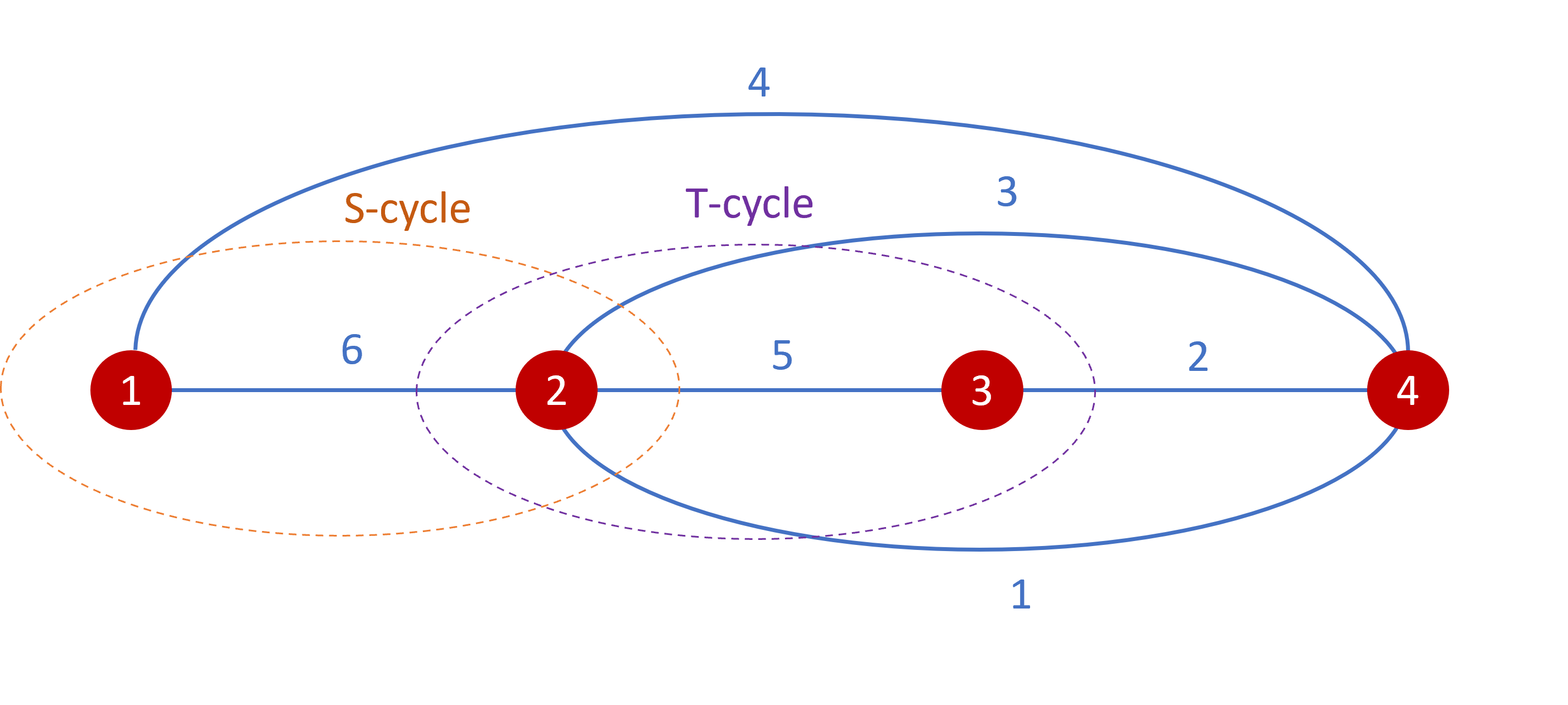
In this section, we study the quantization of SL(2,)\rm{SL}(2,\mathbb{C}) flat connections on 4-holed sphere. The moduli space of SL(2,)\rm{SL}(2,\mathbb{C}) flat connections on nn-holed sphere is a Poisson manifold. A set of useful coordinates are known as the Fock-Goncharov (FG) coordinates, each of which associate to an edge in an ideal triangulation of the nn-holed sphere. See Appendix B for details. FIG.1 is an example of the ideal triangulation of 4-holed sphere. Given any ideal triangulation on nn-holed sphere, we denote the FG coordinate by ze=eZe,z~e=eZ~ez_{e}=e^{Z_{e}},\ \tilde{z}_{e}=e^{\tilde{Z}_{e}}, e=1,,|E|e=1,\cdots,|E| (|E||E| is the number of edges), where Ze,Z~eZ_{e},\tilde{Z}_{e} are lifts of log(ze),log(z~e)\log(z_{e}),\log(\tilde{z}_{e}). We define their classical Poisson bracket by {ze,ze}=2εe,ezeze,{z~e,z~e}=2εe,ez~ez~e\{z_{e},z_{e^{\prime}}\}=2\varepsilon_{e,e^{\prime}}z_{e}z_{e^{\prime}},\ \{\tilde{z}_{e},\tilde{z}_{e^{\prime}}\}=2\varepsilon_{e,e^{\prime}}\tilde{z}_{e}\tilde{z}_{e^{\prime}}. Their quantization [𝑶,𝑶]={O,O}[\bm{O},\bm{O}^{\prime}]=\hbar\{O,O^{\prime}\} and [𝑶~,𝑶~]=~{O~,O~}[\tilde{\bm{O}},\tilde{\bm{O}}^{\prime}]=\tilde{\hbar}\{\tilde{O},\tilde{O}^{\prime}\} leads to the operator algebra

𝒛e𝒛e=𝐪2εe,e𝒛e𝒛e,𝒛~e𝒛~e=𝐪~2εe,e𝒛~e𝒛~e,𝒛e𝒛~e=𝒛~e𝒛e\displaystyle\bm{z}_{e}\bm{z}_{e^{\prime}}=\mathbf{q}^{2\varepsilon_{e,e^{\prime}}}\bm{z}_{e^{\prime}}\bm{z}_{e},\qquad\tilde{\bm{z}}_{e}\tilde{\bm{z}}_{e^{\prime}}=\tilde{\mathbf{q}}^{2\varepsilon_{e,e^{\prime}}}\tilde{\bm{z}}_{e^{\prime}}\tilde{\bm{z}}_{e},\qquad\bm{z}_{e}\tilde{\bm{z}}_{e^{\prime}}=\tilde{\bm{z}}_{e^{\prime}}\bm{z}_{e} (4.1)

εe,e=0,±1,±2\varepsilon_{e,e^{\prime}}=0,\pm 1,\pm 2 counts the number of oriented triangles shared by edges e,ee,e^{\prime}, The contribution from each triangle is +1+1 (1-1) if ee rotates to ee^{\prime} counterclockwisely (clockwisely) in the triangle. εe,e\varepsilon_{e,e^{\prime}} for the triangulation in FIG.1 reads

ε=(010111101000010111101000101000101000).\displaystyle\varepsilon=\left(\begin{array}[]{cccccc}0&-1&0&1&1&-1\\ 1&0&-1&0&0&0\\ 0&1&0&-1&-1&1\\ -1&0&1&0&0&0\\ -1&0&1&0&0&0\\ 1&0&-1&0&0&0\\ \end{array}\right). (4.8)

Similar as the above, we often write ze=e𝒁ez_{e}=e^{\bm{Z}_{e}} and 𝒛~e=e𝒁~e\tilde{\bm{z}}_{e}=e^{\tilde{\bm{Z}}_{e}}. The algebra has centers given by

e𝒛e,e𝒛~e\displaystyle\prod_{e}\bm{z}_{e},\qquad\prod_{e}\tilde{\bm{z}}_{e} (4.9)

where the products are over edges adjacent to a given hole. This quantization can be applied to all ideal triangulations, and different triangulation are associated with different data ({e},εe,e)(\{e\},\varepsilon_{e,e^{\prime}}).

These Poisson bracket defined above can be derived from the Poisson bracket of SL(2,)\mathrm{SL}(2,\mathbb{C}) Chern-Simons theory at level kk. Therefore the operator algebra (4.1) relates to the quantization of SL(2,)\mathrm{SL}(2,\mathbb{C}) Chern-Simons theory on 4-holed sphere.

Refer to caption
Figure 1: An ideal triangulation of a 4-holed sphere, the S-cycle (orange) and T-cycle (purple).

Let us focus on the triangulation in FIG.1. The representation of (4.1) on L2()k\mathcal{H}\simeq L^{2}(\mathbb{R})\otimes\mathbb{C}^{k} can be constructed as the following: Firstly, we relate 𝑿,𝒀\bm{X},\bm{Y} to 𝒁1,𝒁5\bm{Z}_{1},\bm{Z}_{5} by

𝑿+iπ=𝒁1,2𝒀+iπ=𝒁5,i.e.𝒛1=𝒙1,𝒛5=𝒚2.-\bm{X}+i\pi=\bm{Z}_{1},\qquad-2\bm{Y}+i\pi=\bm{Z}_{5},\quad\text{i.e.}\quad\bm{z}_{1}=-\bm{x}^{-1},\qquad\bm{z}_{5}=-\bm{y}^{-2}.

where the representations of 𝒙,𝒚\bm{x},\bm{y} are the same as the above.

𝒚=exp[2πik(ib𝝁𝒎)],𝒙=exp[2πik(ib𝝂𝒏)].\displaystyle\bm{y}=\exp\left[\frac{2\pi i}{k}(-ib\bm{\mu}-\bm{m})\right],\qquad\bm{x}=\exp\left[\frac{2\pi i}{k}(-ib\bm{\nu}-\bm{n})\right].

For the triangulation in FIG.1, the center of the algebra is given by λa2=e2La\lambda_{a}^{2}=e^{2L_{a}}, where

L1\displaystyle-L_{1} =\displaystyle= 12(𝒁4+𝒁62πi),L2=12(𝒁1+𝒁3+𝒁5+𝒁64πi),\displaystyle\frac{1}{2}\left(\bm{Z}_{4}+\bm{Z}_{6}-2\pi i\right),\qquad-L_{2}=\frac{1}{2}\left(\bm{Z}_{1}+\bm{Z}_{3}+\bm{Z}_{5}+\bm{Z}_{6}-4\pi i\right),
L3\displaystyle-L_{3} =\displaystyle= 12(𝒁2+𝒁52πi),L4=12(𝒁1+𝒁2+𝒁3+𝒁44πi).\displaystyle\frac{1}{2}\left(\bm{Z}_{2}+\bm{Z}_{5}-2\pi i\right),\qquad-L_{4}=-\frac{1}{2}\left(\bm{Z}_{1}+\bm{Z}_{2}+\bm{Z}_{3}+\bm{Z}_{4}-4\pi i\right). (4.10)

We may express 𝒁1,,𝒁6\bm{Z}_{1},\cdots,\bm{Z}_{6} in terms of 𝑿,𝒀,L1,,L4\bm{X},\bm{Y},L_{1},\cdots,L_{4}

𝒁1\displaystyle\bm{Z}_{1} =𝑿+iπ,𝒁2=2L3+2𝒀+iπ,\displaystyle=-\bm{X}+i\pi,\qquad\bm{Z}_{2}=-2L_{3}+2\bm{Y}+i\pi,
𝒁3\displaystyle\bm{Z}_{3} =L1L2+L3+L4+𝑿+iπ,\displaystyle=L_{1}-L_{2}+L_{3}+L_{4}+\bm{X}+i\pi,
𝒁4\displaystyle\bm{Z}_{4} =L1+L2+L3+L42𝒀+iπ,𝒁5=2𝒀+iπ,\displaystyle=-L_{1}+L_{2}+L_{3}+L_{4}-2\bm{Y}+i\pi,\qquad\bm{Z}_{5}=-2\bm{Y}+i\pi,
𝒁6\displaystyle\bm{Z}_{6} =L1L2L3L4+2𝒀+iπ\displaystyle=-L_{1}-L_{2}-L_{3}-L_{4}+2\bm{Y}+i\pi (4.11)

We find the representation of all 𝒛e\bm{z}_{e} by

𝒛1\displaystyle\bm{z}_{1} =𝒙1,𝒛2=λ32𝒚2,𝒛3=λ1λ3λ4λ2𝒙,\displaystyle=-\bm{x}^{-1},\qquad\bm{z}_{2}=-\lambda_{3}^{-2}\bm{y}^{2},\qquad\bm{z}_{3}=-\frac{\lambda_{1}\lambda_{3}\lambda_{4}}{\lambda_{2}}\bm{x}, (4.12)
𝒛4\displaystyle\bm{z}_{4} =λ2λ3λ4λ1𝒚2,𝒛5=𝒚2,𝒛6=1λ1λ2λ3λ4𝒚2.\displaystyle=-\frac{\lambda_{2}\lambda_{3}\lambda_{4}}{\lambda_{1}}\bm{y}^{-2},\qquad\bm{z}_{5}=-\bm{y}^{-2},\qquad\bm{z}_{6}=-\frac{1}{\lambda_{1}\lambda_{2}\lambda_{3}\lambda_{4}}\bm{y}^{2}. (4.13)

λ1,,λ6×\lambda_{1},\cdots,\lambda_{6}\in\mathbb{C}^{\times} are constants labelling the representation, and they relate to the centers of the operators algebra of 𝒛e\bm{z}_{e}, e=1,,6e=1,\cdots,6, by

𝒛4𝒛6=λ12,𝒛1𝒛3𝒛5𝒛6=λ22,𝒛2𝒛5=λ32,𝒛1𝒛3𝒛2𝒛4=λ42,\displaystyle\bm{z}_{4}\bm{z}_{6}=\lambda_{1}^{-2},\qquad\bm{z}_{1}\bm{z}_{3}\bm{z}_{5}\bm{z}_{6}=\lambda_{2}^{-2},\qquad\bm{z}_{2}\bm{z}_{5}=\lambda_{3}^{-2},\qquad\bm{z}_{1}\bm{z}_{3}\bm{z}_{2}\bm{z}_{4}=\lambda_{4}^{2}, (4.14)

The tilded operator can be defined similarly

𝒛~1\displaystyle\tilde{\bm{z}}_{1} =𝒙~1,𝒛~2=λ~32𝒚~2,𝒛~3=λ~1λ~3λ~4λ~2𝒙~,\displaystyle=-\tilde{\bm{x}}^{-1},\qquad\tilde{\bm{z}}_{2}=-\tilde{\lambda}_{3}^{-2}\tilde{\bm{y}}^{2},\qquad\tilde{\bm{z}}_{3}=-\frac{\tilde{\lambda}_{1}\tilde{\lambda}_{3}\tilde{\lambda}_{4}}{\tilde{\lambda}_{2}}\tilde{\bm{x}}, (4.15)
𝒛~4\displaystyle\tilde{\bm{z}}_{4} =λ~2λ~3λ~4λ~1𝒚~2,𝒛~5=𝒚~2,𝒛~6=1λ~1λ~2λ~3λ~4𝒚~2.\displaystyle=-\frac{\tilde{\lambda}_{2}\tilde{\lambda}_{3}\tilde{\lambda}_{4}}{\tilde{\lambda}_{1}}\tilde{\bm{y}}^{-2},\qquad\tilde{\bm{z}}_{5}=-\tilde{\bm{y}}^{-2},\qquad\tilde{\bm{z}}_{6}=-\frac{1}{\tilde{\lambda}_{1}\tilde{\lambda}_{2}\tilde{\lambda}_{3}\tilde{\lambda}_{4}}\tilde{\bm{y}}^{2}. (4.16)

where x~,y~\tilde{x},\tilde{y} are represented by

𝒚~=exp[2πik(ib1𝝁+𝒎)],𝒙~=exp[2πik(ib1𝝂+𝒏)].\displaystyle\tilde{\bm{y}}=\exp\left[\frac{2\pi i}{k}(-ib^{-1}\bm{\mu}+\bm{m})\right],\qquad\tilde{\bm{x}}=\exp\left[\frac{2\pi i}{k}(-ib^{-1}\bm{\nu}+\bm{n})\right]. (4.17)

and λ~1,,λ~6×\tilde{\lambda}_{1},\cdots,\tilde{\lambda}_{6}\in\mathbb{C}^{\times} are also constants and label the representation. We set λ~a=λa\tilde{\lambda}_{a}=\lambda_{a}^{*} so that

𝒛e=𝒛~e\displaystyle\bm{z}_{e}^{\dagger}=\tilde{\bm{z}}_{e} (4.18)

representing the star structure. The above representation on \mathcal{H} of the quantum FG coordinates may be denoted by ϱ{λ,λ~}\varrho_{\{\lambda,\tilde{\lambda}\}}, which is labelled by {λ,λ~}{λa,λ~a}a=14\{\lambda,\tilde{\lambda}\}\equiv\{\lambda_{a},\tilde{\lambda}_{a}\}_{a=1}^{4}.

In the following, we mainly focus on the case that k=2Nk=2N is an even number and NN is odd. In this case, we may decompose \mathcal{H} into orthogonal subspaces

+\displaystyle\mathcal{H}\simeq\mathcal{H}_{+}\oplus\mathcal{H}_{-} (4.19)

where ±L2()N\mathcal{H}_{\pm}\simeq L^{2}(\mathbb{R})\otimes\mathbb{C}^{N} contains ϕ±±\phi_{\pm}\in\mathcal{H}_{\pm} satisfying

ϕ±(μ,m+N)=±ϕ±(μ,m).\displaystyle\phi_{\pm}(\mu,m+N)=\pm\phi_{\pm}(\mu,m). (4.20)

±\mathcal{H}_{\pm} is the eigenspace of eπi𝒏e^{\pi i\bm{n}} with eigenvalue ±1\pm 1. The quantization of FG coordinates relates to 𝒙,𝒚2,𝒙~,𝒚~2\bm{x},\bm{y}^{2},\tilde{\bm{x}},\tilde{\bm{y}}^{2}, which act irreducibly on each of +\mathcal{H}_{+} and \mathcal{H}_{-}. The full \mathcal{H} is not irreducible with respect to the quantization of FG coordinates, although it is irreducible with respect to 𝒙,𝒚,𝒙~,𝒚~\bm{x},\bm{y},\tilde{\bm{x}},\tilde{\bm{y}}. Note that the action of 𝒚\bm{y} or 𝒚~\tilde{\bm{y}} maps from +\mathcal{H}_{+} to \mathcal{H}_{-} and vice versa.

4.2 S-cycle trace operator

We define the S-cycle to be the loop enclosing the 1st and 2nd holes (see FIG. 1). Classically, the trace of holonomy along the S-cycle can be written as a function of FG coordinates

Ls\displaystyle L_{s} =\displaystyle= eZ12Z32Z42Z52eZ12+Z32Z42Z52+eZ12+Z42+Z32Z52+eZ12+Z52+Z32+Z42\displaystyle e^{-\frac{Z_{1}}{2}-\frac{Z_{3}}{2}-\frac{Z_{4}}{2}-\frac{Z_{5}}{2}}-e^{-\frac{Z_{1}}{2}+\frac{Z_{3}}{2}-\frac{Z_{4}}{2}-\frac{Z_{5}}{2}}+e^{-\frac{Z_{1}}{2}+\frac{Z_{4}}{2}+\frac{Z_{3}}{2}-\frac{Z_{5}}{2}}+e^{-\frac{Z_{1}}{2}+\frac{Z_{5}}{2}+\frac{Z_{3}}{2}+\frac{Z_{4}}{2}} (4.21)
eZ12+Z42+Z52+Z32+eZ12+Z32+Z42+Z52.\displaystyle-\,e^{-\frac{Z_{1}}{2}+\frac{Z_{4}}{2}+\frac{Z_{5}}{2}+\frac{Z_{3}}{2}}+e^{\frac{Z_{1}}{2}+\frac{Z_{3}}{2}+\frac{Z_{4}}{2}+\frac{Z_{5}}{2}}.

This is derived by using the ”snake rule” outlined in Appendix B. In the language of Teichmüeller theory, LsL_{s} is the complexification of the FN length of the S-cycle, along which the 4-holed sphere is cut into two pairs of pants.

The quantization of the S-cycle trace by Za𝒁aZ_{a}\to\bm{Z}_{a} and inserting (4.1) leads to the operator

𝑳s\displaystyle\bm{L}_{s} =\displaystyle= e2𝒀s+e2𝒀s+eL1L2+L3+L4+2𝒀s+𝑿+eL1L2+𝑿+eL3+L4+𝑿+e2𝒀s+𝑿,\displaystyle e^{-2\bm{Y}_{s}}+e^{2\bm{Y}_{s}}+e^{L_{1}-L_{2}+L_{3}+L_{4}+2\bm{Y}_{s}+\bm{X}}+e^{L_{1}-L_{2}+\bm{X}}+e^{L_{3}+L_{4}+\bm{X}}+e^{-2\bm{Y}_{s}+\bm{X}}, (4.22)
=\displaystyle= e2𝒀s+e2𝒀s+eL3+L4e2𝒀𝐪1(eL1L2L3L4𝐪e2𝒀+1)(1+e2𝒀𝐪)e𝑿,\displaystyle e^{-2\bm{Y}_{s}}+e^{2\bm{Y}_{s}}+e^{L_{3}+L_{4}}e^{-2\bm{Y}}{\bf q}^{-1}\left(e^{L_{1}-L_{2}-L_{3}-L_{4}}{\bf q}e^{2\bm{Y}}+1\right)\left(1+e^{2\bm{Y}}{\bf q}\right)e^{\bm{X}},

where 2𝒀s=2𝒀L3L42\bm{Y}_{s}=2\bm{Y}-L_{3}-L_{4}. Its tilded counter-part 𝑳~s=𝑳s\tilde{\bm{L}}_{s}=\bm{L}_{s}^{\dagger} is obtained analogously

𝑳~s\displaystyle\tilde{\bm{L}}_{s} =\displaystyle= e2𝒀~s+e2𝒀~s+eL~3+L~4e2𝒀~𝐪~1(eL~1L~2L~3L~4𝐪~e2𝒀~+1)(1+e2𝒀~𝐪~)e𝑿~.\displaystyle e^{-2\tilde{\bm{Y}}_{s}}+e^{2\tilde{\bm{Y}}_{s}}+e^{\tilde{L}_{3}+\tilde{L}_{4}}e^{-2\tilde{\bm{Y}}}{\tilde{\mathbf{q}}}^{-1}\left(e^{\tilde{L}_{1}-\tilde{L}_{2}-\tilde{L}_{3}-\tilde{L}_{4}}{\tilde{\mathbf{q}}}e^{2\tilde{\bm{Y}}}+1\right)\left(1+e^{2\tilde{\bm{Y}}}{\tilde{\mathbf{q}}}\right)e^{\tilde{\bm{X}}}. (4.23)

The trace operator 𝑳s\bm{L}_{s} can be simplified by the unitary transformation

𝑼s=φ(y2eL1L2L3L4,y~2eL~1L~2L~3L~4)φ(y2,y~2).\displaystyle\bm{U}^{\prime}_{s}=\varphi\left(y^{2}e^{L_{1}-L_{2}-L_{3}-L_{4}},\tilde{y}^{2}e^{\tilde{L}_{1}-\tilde{L}_{2}-\tilde{L}_{3}-\tilde{L}_{4}}\right)\varphi\left(y^{2},\tilde{y}^{2}\right). (4.24)

Indeed, the recursion relation of the quantum dilogarithm implies the following relation:

𝑼s[eL3+L4e2𝒀𝐪1(eL1L2L3L4𝐪e2𝒀+1)(1+e2𝒀𝐪)e𝑿]𝑼s1=e2𝒀s+𝑿.\displaystyle\bm{U}^{\prime}_{s}\left[e^{L_{3}+L_{4}}e^{-2\bm{Y}}{\bf q}^{-1}\left(e^{L_{1}-L_{2}-L_{3}-L_{4}}{\bf q}e^{2\bm{Y}}+1\right)\left(1+e^{2\bm{Y}}{\bf q}\right)e^{\bm{X}}\right]\bm{U}_{s}^{\prime-1}=e^{-2\bm{Y}_{s}+\bm{X}}. (4.25)

Thereore, we obtain

𝑼s𝑳s𝑼s1=e2𝒀s+e2𝒀s+e2𝒀s+𝑿.\displaystyle\bm{U}^{\prime}_{s}\bm{L}_{s}\bm{U}_{s}^{\prime-1}=e^{-2\bm{Y}_{s}}+e^{2\bm{Y}_{s}}+e^{-2\bm{Y}_{s}+\bm{X}}. (4.26)

The operator can be further simplified by the Weil representation 𝑻\bm{T} of the T-type symplectic transformation 555We refer to [12] for a general discussion of T-type symplectic transformation and its Weil representation as unitary operator.

(YX)(1021)(YX),𝑻=e2πik(𝝁2𝒎2).\displaystyle\left(\begin{array}[]{c}Y\\ X\end{array}\right)\to\begin{pmatrix}1&0\\ -2&1\end{pmatrix}\left(\begin{array}[]{c}Y\\ X\end{array}\right),\qquad\bm{T}=e^{\frac{2\pi i}{k}\left(\bm{\mu}^{2}-\bm{m}^{2}\right)}. (4.31)

The unitary operator 𝑻\bm{T} satisfies

𝑻e𝑿2𝒀𝑻1=e𝑿.\displaystyle\bm{T}e^{\bm{X}-2\bm{Y}}\bm{T}^{-1}=e^{\bm{X}}. (4.32)

As a result, we obtain

𝑳s=𝑼s𝑳s𝑼s1=e2𝒀s+e2𝒀s+e𝑿s,𝑼s=𝑼s𝑻,\displaystyle\bm{L}_{s}^{\prime}=\bm{U}_{s}\bm{L}_{s}\bm{U}_{s}^{-1}=e^{-2\bm{Y}_{s}}+e^{2\bm{Y}_{s}}+e^{\bm{X}_{s}},\qquad\bm{U}_{s}=\bm{U}_{s}^{\prime}\bm{T}, (4.33)

where 𝑿s=𝑿+L3+L4\bm{X}_{s}=\bm{X}+L_{3}+L_{4}. A similar computation shows that 𝑼s\bm{U}_{s} also simplify 𝑳~s\tilde{\bm{L}}_{s}:

𝑳~s=𝑼s𝑳~s𝑼s1=e2𝒀~s+e2𝒀~s+e𝑿~s.\displaystyle\tilde{\bm{L}}_{s}^{\prime}=\bm{U}_{s}\tilde{\bm{L}}_{s}\bm{U}_{s}^{-1}=e^{-2\tilde{\bm{Y}}_{s}}+e^{2\tilde{\bm{Y}}_{s}}+e^{\tilde{\bm{X}}_{s}}. (4.34)

𝑳s,𝑳~s\bm{L}_{s},\tilde{\bm{L}}_{s} can relate to the Casimir operator 𝒬1′′,𝒬~1′′\mathcal{Q}_{1}^{\prime\prime},\tilde{\mathcal{Q}}_{1}^{\prime\prime} in the representation theory of quantum group (recall (3.17) and (3.18)) by unitary transformations. Indeed, we further make a Fourier transform

f(μ,m)=1km/k𝑑μe2πik(μμmm)f(μ,m),f𝔇,\mathcal{F}f(\mu,m)=\frac{1}{k}\sum_{m^{\prime}\in\mathbb{Z}/k\mathbb{Z}}\int d\mu^{\prime}\>e^{\frac{2\pi i}{k}\left(\mu\mu^{\prime}-mm^{\prime}\right)}{f}(\mu^{\prime},m^{\prime}),\qquad\forall\,f\in\mathfrak{D},

such that

1e𝒀=e𝑿,1e𝑿=e𝒀.\displaystyle\mathcal{F}^{-1}e^{\bm{Y}}\mathcal{F}=e^{\bm{X}},\qquad\mathcal{F}^{-1}e^{\bm{X}}\mathcal{F}=e^{-\bm{Y}}. (4.35)

Then

1𝑳s=e2𝑿+L3+L4+e2𝑿L3L4+e𝒀+L3+L4.\displaystyle\mathcal{F}^{-1}\bm{L}_{s}^{\prime}\mathcal{F}=e^{-2{\bm{X}}+L_{3}+L_{4}}+e^{2{\bm{X}}-L_{3}-L_{4}}+e^{-{\bm{Y}}+L_{3}+L_{4}}. (4.36)

Here we assume both eL3,eL4e^{L_{3}},e^{L_{4}} can be parametrized by

eL3=exp[2πik(ibμ3m3)],eL4=exp[2πik(ibμ4m4)]\displaystyle e^{L_{3}}=\exp\left[\frac{2\pi i}{k}\left(-ib\mu_{3}-m_{3}\right)\right],\qquad e^{L_{4}}=\exp\left[\frac{2\pi i}{k}\left(-ib\mu_{4}-m_{4}\right)\right] (4.37)

where μ3,μ4\mu_{3},\mu_{4}\in\mathbb{R} and m3,m4m_{3},m_{4}\in\mathbb{Z}. For this paper, the purpose of this assumption is to simplify some analysis in the following. However, when we consider the quantization of SL(2,)\mathrm{SL}(2,\mathbb{C}) Chern-Simons theory on 3-manifold whose boundary is a closed 2-surface containing the 4-holed sphere as a part of the geodesic boundary (see e.g. [22, 18]), {La}a=14\{L_{a}\}_{a=1}^{4} are part of the Darboux coordinate of the phase space, so {eLa}a=14\{e^{L_{a}}\}_{a=1}^{4} should be quantized in the same way as e𝒀e^{\bm{Y}}.

We apply the unitary shift operator

𝒮34=exp[2πik((μ3+μ4)𝝂(m3+m4)𝒏)]\displaystyle\mathcal{S}_{34}=\exp\left[-\frac{2\pi i}{k}\left((\mu_{3}+\mu_{4})\bm{\nu}-(m_{3}+m_{4})\bm{n}\right)\right] (4.38)

which gives

𝒮34e𝒀+L3+L4𝒮341=e𝒀\displaystyle\mathcal{S}_{34}e^{-{\bm{Y}}+L_{3}+L_{4}}\mathcal{S}_{34}^{-1}=e^{-{\bm{Y}}} (4.39)

similar to (3.16). We obtain

𝒮341𝑳s𝒮341=e2𝑿+L3+L4+e2𝑿L3L4+e𝒀,\displaystyle\mathcal{S}_{34}\mathcal{F}^{-1}\bm{L}_{s}^{\prime}\mathcal{F}\mathcal{S}_{34}^{-1}=e^{-2{\bm{X}}+L_{3}+L_{4}}+e^{2{\bm{X}}-L_{3}-L_{4}}+e^{-{\bm{Y}}}, (4.40)

which relates to 𝒬1′′\mathcal{Q}_{1}^{\prime\prime} by identifying L3+L4L_{3}+L_{4} here to L2L_{2} in 𝒬1′′\mathcal{Q}_{1}^{\prime\prime}. The relation between 𝑳~s\tilde{\bm{L}}_{s}^{\prime} and 𝒬~1′′\tilde{\mathcal{Q}}_{1}^{\prime\prime} is obtained analogously.

If we further assume m3+m42m_{3}+m_{4}\in 2\mathbb{Z}, we can use another unitary shift operator

𝒟34=exp[2πik(μ3+μ42𝝁m3+m42𝒎)]\displaystyle\mathcal{D}_{34}=\exp\left[-\frac{2\pi i}{k}\left(\frac{\mu_{3}+\mu_{4}}{2}\bm{\mu}-\frac{m_{3}+m_{4}}{2}\bm{m}\right)\right] (4.41)

to give

𝒟341e2𝑿L3L4𝒟34=e2𝑿,𝒟341e2𝑿+L3+L4𝒟34=e2𝑿.\displaystyle\mathcal{D}_{34}^{-1}e^{2\bm{X}-L_{3}-L_{4}}\mathcal{D}_{34}=e^{2\bm{X}},\qquad\mathcal{D}_{34}^{-1}e^{-2\bm{X}+L_{3}+L_{4}}\mathcal{D}_{34}=e^{-2\bm{X}}. (4.42)

As a result, the sequence of unitary transformation gives a relatively simple expression of S-cycle trace operator

𝑳s′′=𝒟341𝒮341𝑳s𝒮341𝒟34=e2𝑿+e2𝑿+e𝒀\displaystyle\bm{L}_{s}^{\prime\prime}=\mathcal{D}_{34}^{-1}\mathcal{S}_{34}\mathcal{F}^{-1}\bm{L}_{s}^{\prime}\mathcal{F}\mathcal{S}_{34}^{-1}\mathcal{D}_{34}=e^{-2{\bm{X}}}+e^{2{\bm{X}}}+e^{-{\bm{Y}}} (4.43)
𝑳~s′′=𝒟341𝒮341𝑳~s𝒮341𝒟34=e2𝑿~+e2𝑿~+e𝒀~.\displaystyle\tilde{\bm{L}}_{s}^{\prime\prime}=\mathcal{D}_{34}^{-1}\mathcal{S}_{34}\mathcal{F}^{-1}\tilde{\bm{L}}_{s}^{\prime}\mathcal{F}\mathcal{S}_{34}^{-1}\mathcal{D}_{34}=e^{-2{\tilde{\bm{X}}}}+e^{2\tilde{\bm{X}}}+e^{-\tilde{\bm{Y}}}. (4.44)

In summary, we have made a sequence of unitary transformations

𝔘s=𝒟341𝒮341𝑼s\displaystyle\mathfrak{U}_{s}=\mathcal{D}_{34}^{-1}\mathcal{S}_{34}\mathcal{F}^{-1}\bm{U}_{s} (4.45)

so that

𝑳s′′=𝔘s𝑳s𝔘s1,𝑳~s′′=𝔘s𝑳~s𝔘s1.\displaystyle\bm{L}_{s}^{\prime\prime}=\mathfrak{U}_{s}\bm{L}_{s}\mathfrak{U}_{s}^{-1},\qquad\tilde{\bm{L}}_{s}^{\prime\prime}=\mathfrak{U}_{s}\tilde{\bm{L}}_{s}\mathfrak{U}_{s}^{-1}. (4.46)

4.3 T-cycle trace operator

The operator quantizing the trace of T-cycle enclosing the 2nd and 3rd holes is given by

𝑳t\displaystyle\bm{L}_{t} =\displaystyle= e2𝒀t+e2𝒀t+eL1+L2L3L4𝑿+2𝒀t+eL1L4𝑿+eL2L3𝑿+e𝑿2𝒀t\displaystyle e^{-2\bm{Y}_{t}}+e^{2\bm{Y}_{t}}+e^{-L_{1}+L_{2}-L_{3}-L_{4}-\bm{X}+2\bm{Y}_{t}}+e^{-L_{1}-L_{4}-\bm{X}}+e^{L_{2}-L_{3}-\bm{X}}+e^{-\bm{X}-2\bm{Y}_{t}} (4.47)
=\displaystyle= e2𝒀t+e2𝒀t+eL2+L3𝐪e2𝒀(1+e2L3e2𝒀𝐪1)(1+e(L1+L2+L3+L4)e2𝒀𝐪1)e𝑿\displaystyle e^{-2\bm{Y}_{t}}+e^{2\bm{Y}_{t}}+e^{L_{2}+L_{3}}{\bf q}e^{-2\bm{Y}}\left(1+e^{-2L_{3}}e^{2\bm{Y}}{\bf q}^{-1}\right)\left(1+e^{-\left(L_{1}+L_{2}+L_{3}+L_{4}\right)}e^{2\bm{Y}}{\bf q}^{-1}\right)e^{-\bm{X}}

where 2𝒀t=2𝒀L2L32\bm{Y}_{t}=2\bm{Y}-L_{2}-L_{3}. We obtain the tilded operator by 𝑳~t=𝑳t\tilde{\bm{L}}_{t}=\bm{L}_{t}^{\dagger}. We apply the unitary transformation

𝑼t𝑳t𝑼t1\displaystyle\bm{U}^{\prime}_{t}\bm{L}_{t}\bm{U}^{\prime-1}_{t} =\displaystyle= e2𝒀+L2+L3+e2𝒀L2L3+e2𝒀𝑿+L2+L3,\displaystyle e^{-2\bm{Y}+L_{2}+L_{3}}+e^{2\bm{Y}-L_{2}-L_{3}}+e^{-2\bm{Y}-\bm{X}+L_{2}+L_{3}}, (4.48)

where

𝑼t\displaystyle\bm{U}^{\prime}_{t} =\displaystyle= φ(e(L1+L2+L3+L4)y2,e(L~1+L~2+L~3+L~4)y~2)1φ(e2L3y2,e2L~3y~2)1.\displaystyle\varphi\left(e^{-\left(L_{1}+L_{2}+L_{3}+L_{4}\right)}y^{2},e^{-\left(\tilde{L}_{1}+\tilde{L}_{2}+\tilde{L}_{3}+\tilde{L}_{4}\right)}\tilde{y}^{2}\right)^{-1}\varphi\left(e^{-2L_{3}}y^{2},e^{-2\tilde{L}_{3}}\tilde{y}^{2}\right)^{-1}. (4.49)

The further simplification can be made by the Weil transformation representing the following symplectic transformation

(YX)(1021)(YX)=(1021)(1001)(YX)\displaystyle\left(\begin{array}[]{c}Y\\ X\end{array}\right)\to\begin{pmatrix}-1&0\\ -2&-1\end{pmatrix}\left(\begin{array}[]{c}Y\\ X\end{array}\right)=\begin{pmatrix}1&0\\ 2&1\end{pmatrix}\begin{pmatrix}-1&0\\ 0&-1\end{pmatrix}\left(\begin{array}[]{c}Y\\ X\end{array}\right) (4.56)

We define the unitary operator 𝑽\bm{V} by 𝑽f(μ,m)=f(μ,m)\bm{V}f(\mu,m)=f(-\mu,-m) and obtain

𝑳t=𝑼t𝑳t𝑼t1=e2𝒀L2L3+e2𝒀+L2+L3+e𝑿+L2+L3,𝑼t=𝑻1𝑽𝑼t.\displaystyle\bm{L}_{t}^{\prime}=\bm{U}_{t}\bm{L}_{t}\bm{U}_{t}^{-1}=e^{-2\bm{Y}-L_{2}-L_{3}}+e^{2\bm{Y}+L_{2}+L_{3}}+e^{\bm{X}+L_{2}+L_{3}},\qquad\bm{U}_{t}=\bm{T}^{-1}\bm{V}\bm{U}^{\prime}_{t}. (4.57)

Similar to 𝑳s\bm{L}_{s}, we further make the Fourier transform:

1𝑳t=e2𝑿L2L3+e2𝑿+L2+L3+e𝒀+L2+L3.\displaystyle\mathcal{F}^{-1}\bm{L}_{t}^{\prime}\mathcal{F}=e^{-2{\bm{X}}-L_{2}-L_{3}}+e^{2{\bm{X}}+L_{2}+L_{3}}+e^{-{\bm{Y}}+L_{2}+L_{3}}. (4.58)

If both eL2,eL3e^{L_{2}},e^{L_{3}} can be parametrized by

eL2=exp[2πik(ibμ2m2)],eL3=exp[2πik(ibμ3m3)]\displaystyle e^{L_{2}}=\exp\left[\frac{2\pi i}{k}\left(-ib\mu_{2}-m_{2}\right)\right],\qquad e^{L_{3}}=\exp\left[\frac{2\pi i}{k}\left(-ib\mu_{3}-m_{3}\right)\right] (4.59)

where μ2,μ3\mu_{2},\mu_{3}\in\mathbb{R} and m2,m3m_{2},m_{3}\in\mathbb{Z}. Apply the shift operator

𝒮23=exp[2πik((μ2+μ3)𝝂(m2+m3)𝒏)]\displaystyle\mathcal{S}_{23}=\exp\left[-\frac{2\pi i}{k}\left((\mu_{2}+\mu_{3})\bm{\nu}-(m_{2}+m_{3})\bm{n}\right)\right] (4.60)

which gives

𝒮231𝑳t𝒮231=e2𝑿L2L3+e2𝑿+L2+L3+e𝒀,\displaystyle\mathcal{S}_{23}\mathcal{F}^{-1}\bm{L}_{t}^{\prime}\mathcal{F}\mathcal{S}_{23}^{-1}=e^{-2{\bm{X}}-L_{2}-L_{3}}+e^{2{\bm{X}}+L_{2}+L_{3}}+e^{-{\bm{Y}}}, (4.61)

which relates to 𝒬1′′\mathcal{Q}_{1}^{\prime\prime} by identifying L2L3-L_{2}-L_{3} here to L2L_{2} in 𝒬1′′\mathcal{Q}_{1}^{\prime\prime}.

If we assume m2+m32m_{2}+m_{3}\in 2\mathbb{Z}, we can define another shift operator

𝒟23=exp[2πik(μ2+μ32𝝁m2+m32𝒎)]\displaystyle\mathcal{D}_{23}=\exp\left[-\frac{2\pi i}{k}\left(\frac{\mu_{2}+\mu_{3}}{2}\bm{\mu}-\frac{m_{2}+m_{3}}{2}\bm{m}\right)\right] (4.62)

which gives

𝒟23e2𝑿+L2+L3𝒟231=e2𝑿,𝒟23e2𝑿L2L3𝒟231=e2𝑿.\displaystyle\mathcal{D}_{23}e^{2\bm{X}+L_{2}+L_{3}}\mathcal{D}_{23}^{-1}=e^{2\bm{X}},\qquad\mathcal{D}_{23}e^{-2\bm{X}-L_{2}-L_{3}}\mathcal{D}_{23}^{-1}=e^{-2\bm{X}}. (4.63)

As a result, the sequence of unitary transformation gives same expression as (4.43) for the S-cycle trace operator

𝑳t′′=𝒟23𝒮231𝑳t𝒮231𝒟23=e2𝑿+e2𝑿+e𝒀=𝑳s′′\displaystyle\bm{L}_{t}^{\prime\prime}=\mathcal{D}_{23}\mathcal{S}_{23}\mathcal{F}^{-1}\bm{L}_{t}^{\prime}\mathcal{F}\mathcal{S}_{23}^{-1}\mathcal{D}_{23}=e^{-2{\bm{X}}}+e^{2{\bm{X}}}+e^{-{\bm{Y}}}=\bm{L}_{s}^{\prime\prime} (4.64)
𝑳~t′′=𝒟231𝒮231𝑳~t𝒮231𝒟231=e2𝑿~+e2𝑿~+e𝒀~=𝑳~s′′\displaystyle\tilde{\bm{L}}_{t}^{\prime\prime}=\mathcal{D}_{23}^{-1}\mathcal{S}_{23}\mathcal{F}^{-1}\tilde{\bm{L}}_{t}^{\prime}\mathcal{F}\mathcal{S}_{23}^{-1}\mathcal{D}_{23}^{-1}=e^{-2{\tilde{\bm{X}}}}+e^{2\tilde{\bm{X}}}+e^{-\tilde{\bm{Y}}}=\tilde{\bm{L}}_{s}^{\prime\prime} (4.65)

We denote by

𝔘t=𝒟23𝒮231𝑼t,\displaystyle\mathfrak{U}_{t}=\mathcal{D}_{23}\mathcal{S}_{23}\mathcal{F}^{-1}\bm{U}_{t}, (4.66)

so that

𝑳t′′=𝔘t𝑳t𝔘t1,𝑳~t′′=𝔘t𝑳~t𝔘t1.\displaystyle\bm{L}_{t}^{\prime\prime}=\mathfrak{U}_{t}\bm{L}_{t}\mathfrak{U}_{t}^{-1},\qquad\tilde{\bm{L}}_{t}^{\prime\prime}=\mathfrak{U}_{t}\tilde{\bm{L}}_{t}\mathfrak{U}_{t}^{-1}. (4.67)

Then 𝑳t′′=𝑳s′′\bm{L}_{t}^{\prime\prime}=\bm{L}_{s}^{\prime\prime}, 𝑳~t′′=𝑳~s′′\tilde{\bm{L}}_{t}^{\prime\prime}=\tilde{\bm{L}}_{s}^{\prime\prime} implies that there is a unitary transformation relating (𝑳t,𝑳~t)(\bm{L}_{t},\tilde{\bm{L}}_{t}) and (𝑳s,𝑳~s)(\bm{L}_{s},\tilde{\bm{L}}_{s}).

𝑳s=𝔘s1𝔘t𝑳t𝔘t1𝔘s,𝑳~s=𝔘s1𝔘t𝑳~t𝔘t1𝔘s.\displaystyle\bm{L}_{s}=\mathfrak{U}_{s}^{-1}\mathfrak{U}_{t}\bm{L}_{t}\mathfrak{U}_{t}^{-1}\mathfrak{U}_{s},\qquad\tilde{\bm{L}}_{s}=\mathfrak{U}_{s}^{-1}\mathfrak{U}_{t}\tilde{\bm{L}}_{t}\mathfrak{U}_{t}^{-1}\mathfrak{U}_{s}. (4.68)

Finally, an additional Fourier transform gives the final expression of the trace operator that is studied extensively in the next section

𝑳=𝑳s′′1=e2𝒀+e2𝒀+e𝑿,\displaystyle\bm{L}=\mathcal{F}\bm{L}_{s}^{\prime\prime}\mathcal{F}^{-1}=e^{-2{\bm{Y}}}+e^{2{\bm{Y}}}+e^{{\bm{X}}}, (4.69)
𝑳~=𝑳~s′′1=e2𝒀~+e2𝒀~+e𝑿~.\displaystyle\tilde{\bm{L}}=\mathcal{F}\tilde{\bm{L}}_{s}^{\prime\prime}\mathcal{F}^{-1}=e^{-2\tilde{\bm{Y}}}+e^{2\tilde{\bm{Y}}}+e^{\tilde{\bm{X}}}. (4.70)

The operators 𝑳,𝑳~\bm{L},\tilde{\bm{L}} are generalizations of of the Dehn twist operator of quantum Teichmüller theory studied in [1, 3, 5]. The unitary transformation relating (𝑳s,𝑳~s)(\bm{L}_{s},\tilde{\bm{L}}_{s}) and (𝑳t,𝑳~t)(\bm{L}_{t},\tilde{\bm{L}}_{t}) can be seen as realizing the A-move of Moore-Seiberg groupoid on \mathcal{H}, as a generalization from the result from quantum Teichmüller theory in [6].

The following S-cycle and T-cycle trace operators and their tilded partners are also useful in the following discussion

𝑳s(aux)=e2𝒀+L3+L4+e2𝒀L3L4+e𝑿,\displaystyle\bm{L}_{s}^{(aux)}=e^{-2{\bm{Y}}+L_{3}+L_{4}}+e^{2{\bm{Y}}-L_{3}-L_{4}}+e^{{\bm{X}}}, (4.71)
𝑳t(aux)=e2𝒀L2L3+e2𝒀+L2+L3+e𝑿.\displaystyle\bm{L}_{t}^{(aux)}=e^{-2{\bm{Y}}-L_{2}-L_{3}}+e^{2{\bm{Y}}+L_{2}+L_{3}}+e^{{\bm{X}}}. (4.72)

They are Fourier transforms of (4.40) and (4.61). The derivation of these operator does not rely on the assumption m3+m42m_{3}+m_{4}\in 2\mathbb{Z} or m2+m32m_{2}+m_{3}\in 2\mathbb{Z}, in contrast to 𝑳\bm{L}.

5 Eigenstates of the trace operators

The unbounded operator 𝑳\bm{L} is defined on the domain 𝔇(𝑳)L2()k\mathfrak{D}(\bm{L})\subset\mathcal{H}\simeq L^{2}(\mathbb{R})\otimes\mathbb{C}^{k}. Any functions f(μ,m)f(\mu,m) in 𝔇(𝑳)\mathfrak{D}(\bm{L}) should satisfy

e4πkbμf(μ,m)L2(),e4πkbμf(μ,m)L2(),f(μ+ib,m)L2(),m/k.e^{\frac{4\pi}{k}b\mu}f(\mu,m)\in L^{2}(\mathbb{R}),\qquad e^{-\frac{4\pi}{k}b\mu}f(\mu,m)\in L^{2}(\mathbb{R}),\qquad f(\mu+ib,m)\in L^{2}(\mathbb{R}),\qquad\forall m\in\mathbb{Z}/k\mathbb{Z}.

Recall that Re(b)>0\mathrm{Re}(b)>0, the conditions are satisfied for f(μ,m)f(\mu,m) decaying as fast as e4πk[Re(b)+ϵ]μe^{\mp\frac{4\pi}{k}\left[\mathrm{Re}(b)+\epsilon\right]\mu} (ϵ>0\epsilon>0) when μ±\mu\to\pm\infty and holomorpic in the strip {μIm(μ)[0,Re(b)]}\left\{\mu\in\mathbb{C}\mid\mathrm{Im}(\mu)\in\left[0,\mathrm{Re}(b)\right]\right\} satisfying f(μ+ib,m)L2()f(\mu+ib,m)\in L^{2}(\mathbb{R}). The Hermite functions eμ2/2Hn(μ)e^{-\mu^{2}/2}H_{n}(\mu) , n=1,,n=1,\cdots,\infty satisfy the requirements and make a densed domain in L2()L^{2}(\mathbb{R}). Therefore the domain 𝔇(𝑳)\mathfrak{D}(\bm{L})is dense in L2()kL^{2}(\mathbb{R})\otimes\mathbb{C}^{k}. Similarly, the adjoint 𝑳~=𝑳\tilde{\bm{L}}=\bm{L}^{\dagger} is also densely defined on L2()kL^{2}(\mathbb{R})\otimes\mathbb{C}^{k}. 𝑳{\bm{L}} and its adjoint 𝑳~\tilde{\bm{L}} are commutative.

We would like to solve the eigen-equations:

𝑳αr(μ,m)=(r)αr(μ,m),𝑳~αr(μ,m)=(r)αr(μ,m),(r).\displaystyle\bm{L}\alpha_{r}(\mu,m)=\ell(r)\alpha_{r}(\mu,m),\qquad\tilde{\bm{L}}\alpha_{r}(\mu,m)=\ell(r)^{*}\alpha_{r}(\mu,m),\qquad\ell(r)\in\mathbb{C}.

for some eigenstates αr\alpha_{r}. We can always make the following parametrization of any \ell\in\mathbb{C},

=r+r1,\ell=r+r^{-1},

where r×r\in\mathbb{C}^{\times} is determined by \ell up to a “Weyl refection” rr1r\to r^{-1}.

We consider the following ansatz

αr(μ,m)=φ(𝐪1y2r,𝐪~1y~2r~)φ(𝐪y2r,𝐪~y~2r~)fr(μ,m),\displaystyle\alpha_{r}(\mu,m)=\frac{\varphi\left(-{\bf q}^{-1}y^{2}r,-\tilde{{\bf q}}^{-1}\tilde{y}^{2}\tilde{r}\right)}{\varphi\left(-{\bf q}y^{-2}r,-\tilde{{\bf q}}\tilde{y}^{-2}\tilde{r}\right)}f_{r}(\mu,m), (5.1)

where r,r~r,\tilde{r} are parametrized as the following

r=exp[2πik(ibμrmr)],r~=exp[2πik(ib1μr+mr)]μr,mr/k.\displaystyle r=\exp\left[\frac{2\pi i}{k}(-ib\mu_{r}-m_{r})\right],\qquad\tilde{r}=\exp\left[\frac{2\pi i}{k}(-ib^{-1}\mu_{r}+m_{r})\right]\qquad\mu_{r}\in\mathbb{R},\quad m_{r}\in\mathbb{Z}/k\mathbb{Z}. (5.2)

The eigen-equations implies the following recursion relations of fr(μ,m)f_{r}(\mu,m):

rfr(μ+ib,m1)=fr(μ,m),r~fr(μ+ib1,m+1)=fr(μ,m),\displaystyle rf_{r}(\mu+ib,m-1)=f_{r}(\mu,m),\qquad\tilde{r}f_{r}(\mu+ib^{-1},m+1)=f_{r}(\mu,m), (5.3)

and we find that

fr(μ,m)=e2πik(μrμ+mrm),\displaystyle f_{r}(\mu,m)=e^{-\frac{2\pi i}{k}\left(-\mu_{r}\mu+m_{r}m\right)}, (5.4)

is a solution for any rr. Note that in the above, we have restrict rr to satisfy mr/km_{r}\in\mathbb{Z}/k\mathbb{Z} so that fr(μ,m)f_{r}(\mu,m) is single-valued. As a result, up to a constant rescaling independent of μ,m\mu,m, the following function

αr(μ,m)=e2πik(μrμ+mrm)φ(𝐪1y2r,𝐪~1y~2r~)φ(𝐪y2r,𝐪~y~2r~)\displaystyle\alpha_{r}(\mu,m)=e^{-\frac{2\pi i}{k}\left(-\mu_{r}\mu+m_{r}m\right)}\frac{\varphi\left(-{\bf q}^{-1}y^{2}r,-\tilde{{\bf q}}^{-1}\tilde{y}^{2}\tilde{r}\right)}{\varphi\left(-{\bf q}y^{-2}r,-\tilde{{\bf q}}\tilde{y}^{-2}\tilde{r}\right)} (5.5)

is the eigenstate of 𝑳\bm{L} and 𝑳~\tilde{\bm{L}} corresponding to the eigenvalues r+r1r+r^{-1} and r~+r~1\tilde{r}+\tilde{r}^{-1}.

A similar computation shows that the eignstates of 𝑳s(aux),𝑳~s(aux)\bm{L}^{(aux)}_{s},\tilde{\bm{L}}^{(aux)}_{s} and 𝑳t(aux),𝑳~t(aux)\bm{L}^{(aux)}_{t},\tilde{\bm{L}}^{(aux)}_{t} are given respectively by

αr(s)(μ,m)\displaystyle\alpha_{r}^{(s)}(\mu,m) =\displaystyle= e2πik(μrμ+mrm)φ(𝐪1y2λ31λ41r,𝐪~1y~2λ~31λ~41r~)φ(𝐪y2λ3λ4r,𝐪~y~2λ~3λ~4r~),\displaystyle e^{-\frac{2\pi i}{k}\left(-\mu_{r}\mu+m_{r}m\right)}\frac{\varphi\left(-{\bf q}^{-1}y^{2}\lambda_{3}^{-1}\lambda_{4}^{-1}r,-\tilde{{\bf q}}^{-1}\tilde{y}^{2}\tilde{\lambda}_{3}^{-1}\tilde{\lambda}_{4}^{-1}\tilde{r}\right)}{\varphi\left(-{\bf q}y^{-2}\lambda_{3}\lambda_{4}r,-\tilde{{\bf q}}\tilde{y}^{-2}\tilde{\lambda}_{3}\tilde{\lambda}_{4}\tilde{r}\right)}\ , (5.6)
αr(t)(μ,m)\displaystyle\alpha_{r}^{(t)}(\mu,m) =\displaystyle= e2πik(μrμ+mrm)φ(𝐪1y2λ2λ3r,𝐪~1y~2λ~2λ~3r~)φ(𝐪y2λ21λ31r,𝐪~y~2λ~21λ~31r~).\displaystyle e^{-\frac{2\pi i}{k}\left(-\mu_{r}\mu+m_{r}m\right)}\frac{\varphi\left(-{\bf q}^{-1}y^{2}\lambda_{2}\lambda_{3}r,-\tilde{{\bf q}}^{-1}\tilde{y}^{2}\tilde{\lambda}_{2}\tilde{\lambda}_{3}\tilde{r}\right)}{\varphi\left(-{\bf q}y^{-2}\lambda_{2}^{-1}\lambda_{3}^{-1}r,-\tilde{{\bf q}}\tilde{y}^{-2}\tilde{\lambda}_{2}^{-1}\tilde{\lambda}_{3}^{-1}\tilde{r}\right)}\ . (5.7)
Theorem 5.1.

For k=2Nk=2N with odd NN, the spectral decomposition of (𝐋,𝐋~)(\bm{L},\tilde{\bm{L}}), (𝐋s(aux),𝐋~s(aux))(\bm{L}^{(aux)}_{s},\tilde{\bm{L}}^{(aux)}_{s}), or (𝐋t(aux),𝐋~t(aux))(\bm{L}^{(aux)}_{t},\tilde{\bm{L}}^{(aux)}_{t}) gives the following direct integral representation

mr/k0dμrρ(μr,mr)1μr,mr.\displaystyle\mathcal{H}\simeq\sum_{m_{r}\in\mathbb{Z}/k\mathbb{Z}}\int_{0}^{\infty}\mathrm{d}\mu_{r}\,\rho(\mu_{r},m_{r})^{-1}\,\mathcal{H}_{\mu_{r},m_{r}}. (5.8)

where each μr,mr\mathcal{H}_{\mu_{r},m_{r}} is 1-dimensional, and

ρ(μr,mr)\displaystyle\rho(\mu_{r},m_{r}) =\displaystyle= N2[sin(πN(ibμr+mr))sin(πN(ib1μr+mr))]1\displaystyle N^{2}\left[\sin\left(\frac{\pi}{N}(ib\mu_{r}+m_{r})\right)\sin\left(\frac{\pi}{N}(-ib^{-1}\mu_{r}+m_{r})\right)\right]^{-1} (5.9)

Any ff\in\mathcal{H} can be represented by f(μr,mr)f(\mu_{r},m_{r}) where μr+\mu_{r}\in\mathbb{R}_{+} and mr/km_{r}\in\mathbb{Z}/k\mathbb{Z}, such that 𝐋,𝐋~\bm{L},\tilde{\bm{L}} are represented as the multiplication operators

𝑳f(μr,mr)=(r)f(μr,mr),𝑳~f(μr,mr)=(r)f(μr,mr).\displaystyle\bm{L}f(\mu_{r},m_{r})=\ell(r)f(\mu_{r},m_{r}),\qquad\tilde{\bm{L}}f(\mu_{r},m_{r})=\ell(r)^{*}f(\mu_{r},m_{r}). (5.10)

The same holds for (𝐋s(aux),𝐋~s(aux))(\bm{L}^{(aux)}_{s},\tilde{\bm{L}}^{(aux)}_{s}) or (𝐋t(aux),𝐋~t(aux))(\bm{L}^{(aux)}_{t},\tilde{\bm{L}}^{(aux)}_{t}). For any pair of states f,ff,f^{\prime}\in\mathcal{H}

ff=mr/k0dμrρ(μr,mr)1f(μr,mr)f(μr,mr).\displaystyle\langle f\mid f^{\prime}\rangle=\sum_{m_{r}\in\mathbb{Z}/k\mathbb{Z}}\int_{0}^{\infty}\mathrm{d}\mu_{r}\,\rho(\mu_{r},m_{r})^{-1}f(\mu_{r},m_{r})^{*}f^{\prime}(\mu_{r},m_{r}). (5.11)

We call this direction integral representation the FN representation of SS-cycle or TT-cycle, since the corresponding trace operator is diagonalized.

For k=2Nk=2N with odd NN, we have the decomposition =+\mathcal{H}=\mathcal{H}_{+}\oplus\mathcal{H}_{-}, where f±(μ,m+N)=±f±(μ,m)f_{\pm}(\mu,m+N)=\pm f_{\pm}(\mu,m) for f±±f_{\pm}\in\mathcal{H}_{\pm}. On each of ±\mathcal{H}_{\pm}, 𝒙,𝒚2\bm{x},\bm{y}^{2} are represented as

𝒚2f±(μ,m)=e2πiN(ibμm)f±(μ,m),\displaystyle\bm{y}^{2}f_{\pm}(\mu,m)=e^{\frac{2\pi i}{N}(-ib\mu-m)}f_{\pm}(\mu,m), 𝒙f±(μ,m)=f±(μ+ib,m1),\displaystyle\quad\bm{x}f_{\pm}(\mu,m)=f_{\pm}(\mu+ib,m-1),
𝒚~2f±(μ,m)=e2πiN(ib1μ+m)f±(μ,m),\displaystyle\tilde{\bm{y}}^{2}f_{\pm}(\mu,m)=e^{\frac{2\pi i}{N}(-ib^{-1}\mu+m)}f_{\pm}(\mu,m), 𝒙~f±(μ,m)=f±(μ+ib1,m+1)\displaystyle\quad\tilde{\bm{x}}f_{\pm}(\mu,m)=f_{\pm}(\mu+ib^{-1},m+1) (5.12)

where f±±f_{\pm}\in\mathcal{H}_{\pm} respectively and m/Nm\in\mathbb{Z}/N\mathbb{Z}. 𝑳,𝑳~\bm{L},\tilde{\bm{L}} leave each of +,\mathcal{H}_{+},\mathcal{H}_{-} invariant. Correspondingly, the eigenstate αr\alpha_{r} satisfy

αr(μ,m+N)=(1)mrαr(μ,m),\displaystyle\alpha_{r}(\mu,m+N)=(-1)^{m_{r}}\alpha_{r}(\mu,m), (5.13)

i.e. it is NN-periodic as f+f_{+} (anti-periodic as ff_{-}) when mrm_{r} is even (odd).

±\mathcal{H}_{\pm} as subspaces of \mathcal{H} have the inner products inherited from \mathcal{H}. Since ±L2()N\mathcal{H}_{\pm}\simeq L^{2}(\mathbb{R})\otimes\mathbb{C}^{N} It is also helpful to consider a different inner product on ±\mathcal{H}_{\pm}:

f±f±N=m/Ndμf±(μ,m)f±(μ,m)=12f±f±.\displaystyle\langle f_{\pm}\mid f^{\prime}_{\pm}\rangle_{N}=\sum_{m\in\mathbb{Z}/N\mathbb{Z}}\int\mathrm{d}\mu\,f_{\pm}(\mu,m)^{*}f^{\prime}_{\pm}(\mu,m)=\frac{1}{2}\langle f_{\pm}\mid f^{\prime}_{\pm}\rangle. (5.14)

Since all 𝑳,𝑳~\bm{L},\tilde{\bm{L}}, (𝑳s(aux),𝑳~s(aux))(\bm{L}^{(aux)}_{s},\tilde{\bm{L}}^{(aux)}_{s}), and (𝑳t(aux),𝑳~t(aux))(\bm{L}^{(aux)}_{t},\tilde{\bm{L}}^{(aux)}_{t}) leave each of +,\mathcal{H}_{+},\mathcal{H}_{-} invariant, we prove Theorem 5.1 by studying the spectral decompostion in +\mathcal{H}_{+} and \mathcal{H}_{-} separately. The following proof mainly focuses on the spectral decomposition of 𝑳,𝑳~\bm{L},\tilde{\bm{L}}. The proof for 𝑳s(aux),𝑳~s(aux)\bm{L}^{(aux)}_{s},\tilde{\bm{L}}^{(aux)}_{s} and 𝑳t(aux),𝑳~t(aux)\bm{L}^{(aux)}_{t},\tilde{\bm{L}}^{(aux)}_{t} can be obtained analogously.

5.1 Periodic states

We firstly restrict to the subset of eigenstates αr\alpha_{r} with even mrm_{r}. In this case, we can express αr\alpha_{r} in terms of γ(x,n)=Db(x,n)\gamma(x,n)={\rm D}_{b}(-x,n), where Db{\rm D}_{b} is the quantum dilogarithm function studied in [11, 10] (see Appendix A for some useful properties):

γ(x,n)\displaystyle\gamma(-x,n) =\displaystyle= Db(x,n)=j=01𝐪2j+1exp[2πiN(ibxN+n)]1𝐪~2j1exp[2πiN(ib1xNn)],\displaystyle{\rm D}_{b}(x,n)=\prod_{j=0}^{\infty}\frac{1-{\bf q}^{2j+1}\exp\left[\frac{2\pi i}{N}\left(-ibx\sqrt{N}+n\right)\right]}{1-\tilde{{\bf q}}^{-2j-1}\exp\left[\frac{2\pi i}{N}\left(-ib^{-1}x\sqrt{N}-n\right)\right]}, (5.15)
𝐪\displaystyle{\bf q} =\displaystyle= eπiN(1+b2),𝐪~=eπiN(1+b2),\displaystyle e^{\frac{\pi i}{N}(1+b^{2})},\qquad\tilde{{\bf q}}=e^{\frac{\pi i}{N}(1+b^{-2})}, (5.16)

and Db\mathrm{D}_{b} relates to φ\varphi by

φ(y2,y~2)=Db(μN,m)1=γ(μN,m)1.\displaystyle\varphi\left(-y^{2},-\tilde{y}^{2}\right)=\mathrm{D}_{b}\left(\frac{\mu}{\sqrt{N}},-m\right)^{-1}=\gamma\left(-\frac{\mu}{\sqrt{N}},-m\right)^{-1}. (5.17)

The expression of αr\alpha_{r} is given by

αr(μ,m)=eπiN[mrmμrμ]γ(μr/2μ+cbN,mmr/2)γ(μr/2+μcbN,mmr/2),cb=i2(b+b1).\displaystyle\alpha_{r}(\mu,m)=e^{-\frac{\pi i}{N}\left[m_{r}m-\mu_{r}\mu\right]}\frac{\gamma\left(-\frac{\mu_{r}/2-\mu+c_{b}}{\sqrt{N}},m-m_{r}/2\right)}{\gamma\left(-\frac{\mu_{r}/2+\mu-c_{b}}{\sqrt{N}},-m-m_{r}/2\right)},\qquad c_{b}=\frac{i}{2}(b+b^{-1}). (5.18)

αr\alpha_{r} has poles along the real μ\mu axis, so we propose a regularization by shifting μμ+iϵN\mu\to\mu+i\epsilon\sqrt{N} with ϵ>0\epsilon>0 inside γ\gamma. Moreover, if we multiply αr\alpha_{r} by a factor βr\beta_{r} independent of μ,m\mu,m

ψr=βrαr,βr=exp(iπcb23NiπcbμrN+iπmr2+iπμr24NiπN6),\displaystyle\psi_{r}=\beta_{r}\alpha_{r},\qquad\beta_{r}=\exp\left(-\frac{i\pi c_{b}^{2}}{3N}-\frac{i\pi c_{b}\mu_{r}}{N}+\frac{i\pi m_{r}}{2}+\frac{i\pi\mu_{r}^{2}}{4N}-\frac{i\pi N}{6}\right), (5.19)

ψr\psi_{r} is manifestly invariant under the Weyl reflection rr1r\to r^{-1} (recall that the eigenvalue is invariant under the reflection ):

ψr=ψr1.\displaystyle\psi_{r}=\psi_{r^{-1}}. (5.20)

Indeed, we introduce some short-hand notations 666These notations are inspired by [7].

ω=i2bN,ω=ib2N,ω′′=cbN,x=μN,λ=μr2N.\displaystyle\omega=\frac{i}{2b\sqrt{N}},\quad\omega^{\prime}=\frac{ib}{2\sqrt{N}},\quad\omega^{\prime\prime}=\frac{c_{b}}{\sqrt{N}},\quad x=\frac{\mu}{\sqrt{N}},\quad\lambda=\frac{\mu_{r}}{2\sqrt{N}}. (5.21)

and apply the inverse relation γ(x,n)γ(x,n)=exp(iπn2NiπniπN6+iπx213iπω′′)2\gamma(x,n)\gamma(-x,-n)=\exp(-\frac{i\pi n^{2}}{N}-i\pi n-\frac{i\pi N}{6}+i\pi x^{2}-\frac{1}{3}i\pi\omega^{\prime\prime}{}^{2}) to αr\alpha_{r}, and we obtain

ψr(μ,m)\displaystyle\psi_{r}(\mu,m) =\displaystyle= eiπm2N+iπmr24Niπmiπ(x+iϵω′′)2\displaystyle e^{\frac{i\pi m^{2}}{N}+\frac{i\pi m_{r}^{2}}{4N}-i\pi m-i\pi\left(x+i\epsilon-\omega^{\prime\prime}\right)^{2}} (5.22)
γ(λ+xω′′+iϵ,mmr2)γ(λ+xω′′+iϵ,m+mr2)\displaystyle\gamma\left(-\lambda+x-\omega^{\prime\prime}+i\epsilon,m-\frac{m_{r}}{2}\right)\gamma\left(\lambda+x-\omega^{\prime\prime}+i\epsilon,m+\frac{m_{r}}{2}\right)

which is manifestly invariant under (λ,mr)(λ,mr)(\lambda,m_{r})\to(-\lambda,-m_{r}) 777A similar computation re-scales αr(s),αr(t)\alpha_{r}^{(s)},\alpha_{r}^{(t)} to ψr(s),ψr(t)\psi_{r}^{(s)},\psi_{r}^{(t)}, where ψr(s)\displaystyle\psi_{r}^{(s)} =\displaystyle= eiπmr24N+iπ(mm32m42)2Niπ(mm32m42)iπ(xω′′+iϵ)2\displaystyle e^{\frac{i\pi m_{r}^{2}}{4N}+\frac{i\pi\left(m-\frac{m_{3}}{2}-\frac{m_{4}}{2}\right){}^{2}}{N}-i\pi\left(m-\frac{m_{3}}{2}-\frac{m_{4}}{2}\right)-i\pi\left(x-\omega^{\prime\prime}+i\epsilon\right)^{2}} (5.23) γ(λ+xω′′+iϵ,mr2+mm32m42)γ(λ+xω′′+iϵ,mr2+mm32m42)\displaystyle\gamma\left(-\lambda+x-\omega^{\prime\prime}+i\epsilon,-\frac{m_{r}}{2}+m-\frac{m_{3}}{2}-\frac{m_{4}}{2}\right)\gamma\left(\lambda+x-\omega^{\prime\prime}+i\epsilon,\frac{m_{r}}{2}+m-\frac{m_{3}}{2}-\frac{m_{4}}{2}\right) up to a constant shift of xx, and ψr(t)\psi_{r}^{(t)} is given by m3m2,m4m3m_{3}\to-m_{2},\ m_{4}\to-m_{3}. Both ψr(s)\psi_{r}^{(s)} and ψr(t)\psi_{r}^{(t)} are invariant under (λ,mr)(λ,mr)(\lambda,m_{r})\to(-\lambda,-m_{r}).. We often fix the symmetry by requiring λ0\lambda\geq 0 (μr0\mu_{r}\geq 0).

The following two lemmas state that ψr\psi_{r} for even mrm_{r} form a complete distributional orthogonal basis for +\mathcal{H}_{+}.

Lemma 5.2.

The eigenstates with even mrm_{r} satisfy the following orthogonality

ψrψrN=12ψrψr=12ρ(μr,mr)δr,r.\displaystyle\left\langle\psi_{r}\mid\psi_{r^{\prime}}\right\rangle_{N}=\frac{1}{2}\left\langle\psi_{r}\mid\psi_{r^{\prime}}\right\rangle=\frac{1}{2}\rho(\mu_{r},m_{r})\delta_{r,r^{\prime}}. (5.24)

where

δr,r\displaystyle\delta_{r,r^{\prime}} =\displaystyle= 12[δ(μrμr)δmr,mr+δ(μr+μr)δmr,mr].\displaystyle\frac{1}{2}\left[\delta(\mu_{r}-\mu_{r^{\prime}})\delta_{m_{r},m_{r^{\prime}}}+\delta(\mu_{r}+\mu_{r^{\prime}})\delta_{m_{r},-m_{r^{\prime}}}\right]. (5.25)
Proof.

First of all, by the periodicity of ψr\psi_{r}, we have

m/kdμψr(μ,m)ψr(μ,m)=2m/Ndμψr(μ,m)ψr(μ,m).\displaystyle\sum_{m\in\mathbb{Z}/k\mathbb{Z}}\int\mathrm{d}\mu\,\psi_{r}(\mu,m)^{*}\psi_{r^{\prime}}(\mu,m)=2\sum_{m\in\mathbb{Z}/N\mathbb{Z}}\int\mathrm{d}\mu\,\psi_{r}(\mu,m)^{*}\psi_{r^{\prime}}(\mu,m). (5.26)

The integrand ψr(μ,m)ψr(μ,m)\psi_{r}(\mu,m)^{*}\psi_{r^{\prime}}(\mu,m) is given by

eiπ(mr2mr2)4N+4iπx(ω′′iϵ)γ(λ+xω′′+iϵ,mmr2)γ(λ+xω′′+iϵ,m+mr2)γ(λ+x+ω′′iϵ,mmr2)γ(λ+x+ω′′iϵ,mr2+m),\displaystyle e^{-\frac{i\pi(m_{r}^{2}-m_{r^{\prime}}^{2})}{4N}+4i\pi x(\omega^{\prime\prime}-i\epsilon)}\frac{\gamma\left(-\lambda^{\prime}+x-\omega^{\prime\prime}+i\epsilon,m-\frac{m_{r^{\prime}}}{2}\right)\gamma\left(\lambda^{\prime}+x-\omega^{\prime\prime}+i\epsilon,m+\frac{m_{r^{\prime}}}{2}\right)}{\gamma\left(-\lambda+x+\omega^{\prime\prime}-i\epsilon,m-\frac{m_{r}}{2}\right)\gamma\left(\lambda+x+\omega^{\prime\prime}-i\epsilon,\frac{m_{r}}{2}+m\right)}, (5.27)

where λ=μr/2N\lambda^{\prime}={\mu_{r^{\prime}}}/{2\sqrt{N}}. We use the integration identity (A.17) to transform the ratio of two γ\gamma’s 888The variables involved in (A.17) are given by t=xt=x, α=λω′′+iϵ,β=λ+ω′′iϵ\alpha=\lambda^{\prime}-\omega^{\prime\prime}+i\epsilon,\ \beta=\lambda^{\prime}+\omega^{\prime\prime}-i\epsilon, d=md=m, a=mr/2a=m_{r}^{\prime}/2, and p=mr/2p=m_{r}/2. We have Im(α+cbN)=ϵ>0,Im(cbNβ)=ϵ>0,Im(αβ)=2ϵb+b1N<0\mathrm{Im}\left(\alpha+\frac{c_{b}}{\sqrt{N}}\right)=\epsilon>0,\ \mathrm{Im}\left(\frac{c_{b}}{\sqrt{N}}-\beta\right)=\epsilon>0,\ \mathrm{Im}(\alpha-\beta)=2\epsilon-\frac{b+b^{-1}}{\sqrt{N}}<0 for sufficiently small ϵ>0\epsilon>0. Therefore there exist an integration contour of ss with Im(αβ)<Im(s)<0\mathrm{Im}(\alpha-\beta)<\mathrm{Im}(s)<0 allowing (A.17) to hold.

γ(λ+xω′′+iϵ,m+mr2)γ(λ+x+ω′′iϵ,mr2+m)\displaystyle\frac{\gamma\left(\lambda^{\prime}+x-\omega^{\prime\prime}+i\epsilon,m+\frac{m_{r^{\prime}}}{2}\right)}{\gamma\left(\lambda+x+\omega^{\prime\prime}-i\epsilon,\frac{m_{r}}{2}+m\right)} (5.28)
=\displaystyle= ζ0Nc/Ndse2iπc(m+mr/2)N+2iπs(x+λ)γ(λ+λ+s+ω′′2iϵ,cmr2+mr2)γ(s+ω′′,c)γ(λ+λ+ω′′2iϵ,mr2mr2),\displaystyle\frac{\zeta_{0}}{\sqrt{N}}\sum_{c\in\mathbb{Z}/N\mathbb{Z}}\int\mathrm{d}s\frac{e^{\frac{2i\pi c(m+m_{r^{\prime}}/2)}{N}+2i\pi s(x+\lambda^{\prime})}\gamma\left(-\lambda^{\prime}+\lambda+s+\omega^{\prime\prime}-2i\epsilon,-c-\frac{m_{r^{\prime}}}{2}+\frac{m_{r}}{2}\right)}{\gamma\left(s+\omega^{\prime\prime},-c\right)\gamma\left(-\lambda^{\prime}+\lambda+\omega^{\prime\prime}-2i\epsilon,\frac{m_{r}}{2}-\frac{m_{r^{\prime}}}{2}\right)},

where ζ0=e112iπ(N4cb2/N)\zeta_{0}=e^{-\frac{1}{12}i\pi\left(N-4c_{b}^{2}/N\right)}.

Inserting (5.28) in (5.27), we check that the integrand of dμds\int\mathrm{d}\mu\mathrm{d}s is a Schwarz function on 2\mathbb{R}^{2} 999The integrand suppresses exponentially fast as μ,Re(s)\mu,\mathrm{Re}(s)\to\infty, as can be shown by using Db(cbN+x,n)exp[iπ(x+cbN)2+O(1)]{\rm D}_{b}(\frac{c_{b}}{\sqrt{N}}+x,n)\sim\exp\left[i\pi\left(x+\frac{c_{b}}{\sqrt{N}}\right)^{2}+O(1)\right] as Re(x)\mathrm{Re}(x)\to\infty and Db(cbN+x,n)O(1){\rm D}_{b}(\frac{c_{b}}{\sqrt{N}}+x,n)\sim O(1) as Re(x)\mathrm{Re}(x)\to-\infty [12]. , so we can interchange the order of integration. Then we compute the integral and sum of μ=xN,m/N\mu=x\sqrt{N},m\in\mathbb{Z}/N\mathbb{Z} by applying (A.15) 101010 We replace the variables in (A.15) by tx,αλω′′+2iϵ,βλ+ω′′2iϵ,ss+2iϵ2ω′′,amr/2,pmr/2,cct\to x,\ \alpha\to-\lambda^{\prime}-\omega^{\prime\prime}+2i\epsilon,\ \beta\to-\lambda+\omega^{\prime\prime}-2i\epsilon,\ s\to-s+2i\epsilon-2\omega^{\prime\prime},\ a\to-m_{r}^{\prime}/2,\ p\to-m_{r}/2,\ c\to-c (the left-hand sides are variables in (A.15), while the right-hand sides are variables in (5.28)). We have Im(α+cbN)ϵ>0,Im(cbNβ)ϵ>0,Im(αβ)2ϵb+b1N<0\mathrm{Im}\left(\alpha+\frac{c_{b}}{\sqrt{N}}\right)\to\epsilon>0,\ \mathrm{Im}\left(\frac{c_{b}}{\sqrt{N}}-\beta\right)\to\epsilon>0,\ \mathrm{Im}(\alpha-\beta)\to 2\epsilon-\frac{b+b^{-1}}{\sqrt{N}}<0 for sufficiently small ϵ>0\epsilon>0, and Im(s)2ϵb+b1NIm(s)\mathrm{Im}(s)\to 2\epsilon-\frac{b+b^{-1}}{\sqrt{N}}-\mathrm{Im}(s). Therefore for sufficiently small ϵ>0\epsilon>0, Im(s)<0\mathrm{Im}(s)<0 and small |Im(s)||\mathrm{Im}(s)| in (5.28) implies Im(αβ)<Im(s)<0\mathrm{Im}(\alpha-\beta)<\mathrm{Im}(s)<0 in (A.15), ensuring the validity of (A.15). then using the inverse formula and recusion relation of γ\gamma. We obtain that as ϵ0\epsilon\to 0

m/Ndμψr(μ,m)ψr(μ,m)\displaystyle\sum_{m\in\mathbb{Z}/N\mathbb{Z}}\int\mathrm{d}\mu\,\psi_{r}(\mu,m)^{*}\psi_{r^{\prime}}(\mu,m) =\displaystyle= 12Nρ(μr,mr)c/Ndse2πiNc(mr2+mr2)+2iπs(λ+λ)\displaystyle\frac{1}{2\sqrt{N}}\rho(\mu_{r},m_{r})\sum_{c\in\mathbb{Z}/N\mathbb{Z}}\int\mathrm{d}s\,e^{-\frac{2\pi i}{N}c\left(\frac{m_{r^{\prime}}}{2}+\frac{m_{r}}{2}\right)+2i\pi s\left(\lambda^{\prime}+\lambda\right)} (5.29)
=\displaystyle= 12ρ(μr,mr)δ(μr+μr)δmr+mr,0.\displaystyle\frac{1}{2}\rho(\mu_{r},m_{r})\delta(\mu_{r}+\mu_{r^{\prime}})\delta_{m_{r}+m_{r^{\prime}},0}\ .

This equation holds in the sense of tempered distribution111111The result of ss-integral is understood as a tempered distribution, which makes sense only when interring another integral, say, over μr=2Nλr\mu_{r}=2\sqrt{N}\lambda_{r}. For finite ϵ\epsilon, the integrand of ds\int\mathrm{d}s is e2πiNc(mr2+mr2)+2iπs(λ+λ)e^{-\frac{2\pi i}{N}c\left(\frac{m_{r^{\prime}}}{2}+\frac{m_{r}}{2}\right)+2i\pi s\left(\lambda^{\prime}+\lambda\right)} multiply a Schwarz function in ss. Consider the following integral: dxdke2πik(xx)fϵ(k)F(x)\int\mathrm{d}x\mathrm{d}k\ e^{2\pi ik(x-x^{\prime})}f_{\epsilon}(k)F(x) with both fϵ,Ff_{\epsilon},F Schwarz functions and limϵ0fϵ(k)=1\lim_{\epsilon\to 0}f_{\epsilon}(k)=1. This integral equals dke2πikxfϵ(k)F~(k)=f(x)\int\mathrm{d}k\,e^{-2\pi ikx^{\prime}}f_{\epsilon}(k)\widetilde{F}(k)=f(x^{\prime}) as ϵ0\epsilon\to 0, where the limit and integral can be interchanged by the dominant convergence. The computation in (5.29) is the same.. Finally, using the reflection symmetry of ψr\psi_{r}

m/kdμψr(μ,m)ψr(μ,m)\displaystyle\sum_{m\in\mathbb{Z}/k\mathbb{Z}}\int\mathrm{d}\mu\,\psi_{r}(\mu,m)^{*}\psi_{r^{\prime}}(\mu,m) =\displaystyle= 12m/kdμψr(μ,m)[ψr(μ,m)+ψr1(μ,m)]\displaystyle\frac{1}{2}\sum_{m\in\mathbb{Z}/k\mathbb{Z}}\int\mathrm{d}\mu\,\psi_{r}(\mu,m)^{*}\left[\psi_{r^{\prime}}(\mu,m)+\psi_{r^{\prime}{}^{-1}}(\mu,m)\right] (5.30)
=\displaystyle= ρ(μr,mr)δr,r\displaystyle\rho(\mu_{r},m_{r})\,\delta_{r,r^{\prime}}

Lemma 5.3.

The eigenstates satisfy the following resolution of identity on +\mathcal{H}_{+}

2mr/2/N0dμrρ(μr,mr)1ψr(μ,m)ψr(μ,m)=δ(μ,μ)δm,m.\displaystyle 2\sum_{m_{r}/2\in\mathbb{Z}/N\mathbb{Z}}\int_{0}^{\infty}\mathrm{d}\mu_{r}\,\rho(\mu_{r},m_{r})^{-1}\,\psi_{r}(\mu^{\prime},m^{\prime})\,\psi_{r}(\mu,m)^{*}=\delta(\mu,\mu^{\prime})\,\delta_{m,m^{\prime}}. (5.31)

for μ,μ\mu,\mu^{\prime}\in\mathbb{R} and m,m/Nm,m^{\prime}\in\mathbb{Z}/N\mathbb{Z}.

Proof.

Firstly we define σ(μr,mr)\sigma(\mu_{r},m_{r}) such that ρ(μr,mr)1=σ(μr,mr)+σ(μr,mr)\rho(\mu_{r},m_{r})^{-1}=\sigma(\mu_{r},m_{r})+\sigma(-\mu_{r},-m_{r}):

σ(μr,mr)=e4iπλω′′eiπmrN+4iπmrω24iπmrωω′′e4iπλ(ω′′2ω)eiπmrN+4iπmrω24iπmrωω′′4N2,\displaystyle\sigma(\mu_{r},m_{r})=\frac{e^{-4i\pi\lambda\omega^{\prime\prime}}e^{-\frac{i\pi m_{r}}{N}+4i\pi m_{r}\omega^{\prime}{}^{2}-4i\pi m_{r}\omega^{\prime}{}\omega^{\prime\prime}}-e^{-4i\pi\lambda(\omega^{\prime\prime}-2\omega^{\prime}{})}e^{\frac{i\pi m_{r}}{N}+4i\pi m_{r}\omega^{\prime}{}^{2}-4i\pi m_{r}\omega^{\prime}{}\omega^{\prime\prime}}}{4N^{2}}, (5.32)

so that

mr/2/Ndμrσ(μr,mr)ψr(μ,m)ψr(μ,m)\displaystyle\sum_{m_{r}/2\in\mathbb{Z}/N\mathbb{Z}}\int_{-\infty}^{\infty}\mathrm{d}\mu_{r}\,\sigma(\mu_{r},m_{r})\,\psi_{r}(\mu^{\prime},m^{\prime})\,\psi_{r}(\mu,m)^{*} =\displaystyle= mr/2/N0dμrρ(μr,mr)1ψr(μ,m)ψr(μ,m).\displaystyle\sum_{m_{r}/2\in\mathbb{Z}/N\mathbb{Z}}\int_{0}^{\infty}\mathrm{d}\mu_{r}\,\rho(\mu_{r},m_{r})^{-1}\,\psi_{r}(\mu^{\prime},m^{\prime})\,\psi_{r}(\mu,m)^{*}.

We consider the integral

I\displaystyle I =\displaystyle= mr/2/Ndμrσ(μr,mr)ψr(μ,m)ψr(μ,m)\displaystyle\sum_{m_{r}/2\in\mathbb{Z}/N\mathbb{Z}}\int_{-\infty}^{\infty}\mathrm{d}\mu_{r}\,\sigma(\mu_{r},m_{r})\,\psi_{r}(\mu^{\prime},m^{\prime})\,\psi_{r}(\mu,m)^{*} (5.33)
=\displaystyle= 2Nmr/2/Ndλσeiπ(m2m2)N+iπ(mm)+iπ(x2y2)+2iπ(x+y)ω′′\displaystyle 2\sqrt{N}\sum_{m_{r}/2\in\mathbb{Z}/N\mathbb{Z}}\int_{-\infty}^{\infty}\mathrm{d}\lambda\,\sigma\,e^{-\frac{i\pi\left(m^{2}-{m^{\prime}}^{2}\right)}{N}+i\pi(m-{m^{\prime}})+i\pi\left(x^{2}-y^{2}\right)+2i\pi(x+y)\omega^{\prime\prime}}
γ(λω′′+y+iϵ,mmr2)γ(λω′′+y+iϵ,mr2+m)γ(λ+x+ω′′iϵ,mmr2)γ(λ+x+ω′′iϵ,mr2+m),\displaystyle\frac{\gamma\left(-\lambda-\omega^{\prime\prime}+y+i\epsilon,m^{\prime}-\frac{m_{r}}{2}\right)\gamma\left(\lambda-\omega^{\prime\prime}+y+i\epsilon,\frac{m_{r}}{2}+m^{\prime}\right)}{\gamma\left(-\lambda+x+\omega^{\prime\prime}-i\epsilon,m-\frac{m_{r}}{2}\right)\gamma\left(\lambda+x+\omega^{\prime\prime}-i\epsilon,\frac{m_{r}}{2}+m\right)},

and we make the following change of variables

t=λ,α=ω′′+y+iϵ,β=x+ω′′iϵ,a=m,p=m,d=mr2.\displaystyle-t=\lambda,\qquad\alpha=-\omega^{\prime\prime}+y+i\epsilon,\qquad\beta=x+\omega^{\prime\prime}-i\epsilon,\qquad a=m^{\prime},\qquad p=m,\qquad-d=\frac{m_{r}}{2}. (5.34)

Then we apply (A.17) for Im(α+cbN)=Im(β+cbN)=ϵ>0\mathrm{Im}(\alpha+\frac{c_{b}}{\sqrt{N}})=\mathrm{Im}(-\beta+\frac{c_{b}}{\sqrt{N}})=\epsilon>0 and Im(αβ)=2ϵ2Im(cb)N<Im(s)<0\mathrm{Im}(\alpha-\beta)=2\epsilon-\frac{2\mathrm{Im}(c_{b})}{\sqrt{N}}<\mathrm{Im}(s)<0. The result is

I=I1+I2\displaystyle I=I_{1}+I_{2} (5.35)

where I1,I2I_{1},I_{2} correspond to two terms in σ(μr,mr)\sigma(\mu_{r},m_{r}),

I1\displaystyle I_{1} =\displaystyle= ζ02N2d,c/Ndtdseiπ(α2β2)+iπ(a2+2acp2)Niπ(ap)2iπNdc\displaystyle\frac{\zeta_{0}}{2N^{2}}\sum_{d,c\in\mathbb{Z}/N\mathbb{Z}}\int\mathrm{d}t\mathrm{d}s\,e^{-i\pi\left(\alpha^{2}-\beta^{2}\right)+\frac{i\pi\left(a^{2}+2ac-p^{2}\right)}{N}-i\pi(a-p)-\frac{2i\pi}{N}dc} (5.36)
e2iπs(α+ω′′)2iπt(s2ω′′)γ(α+t,a+d)γ(α+β+sω′′,ac+p)γ(s+ω′′,c)γ(β+t,d+p)γ(α+βω′′,pa),\displaystyle e^{2i\pi s\left(\alpha+\omega^{\prime\prime}\right)-2i\pi t(s-2\omega^{\prime\prime})}\frac{\gamma(\alpha+t,a+d)\gamma\left(-\alpha+\beta+s-\omega^{\prime\prime},-a-c+p\right)}{\gamma\left(s+\omega^{\prime\prime},-c\right)\gamma(\beta+t,d+p)\gamma\left(-\alpha+\beta-\omega^{\prime\prime},p-a\right)},

and

I2\displaystyle I_{2} =\displaystyle= ζ02N2d,c/Ndtdseiπ(α2β2)+iπ(a2+2acp2)Niπ(ap)2iπNd(c+2)\displaystyle-\frac{\zeta_{0}}{2N^{2}}\sum_{d,c\in\mathbb{Z}/N\mathbb{Z}}\int\mathrm{d}t\mathrm{d}s\,e^{-i\pi\left(\alpha^{2}-\beta^{2}\right)+\frac{i\pi\left(a^{2}+2ac-p^{2}\right)}{N}-i\pi(a-p)-\frac{2i\pi}{N}d\left(c+2\right)} (5.37)
e2iπs(α+ω′′)2iπt(s2ω+2ω)γ(α+t,a+d)γ(α+β+sω′′,ac+p)γ(s+ω′′,c)γ(β+t,d+p)γ(α+βω′′,pa).\displaystyle e^{2i\pi s\left(\alpha+\omega^{\prime\prime}\right)-2i\pi t\left(s-2\omega+2\omega^{\prime}\right)}\frac{\gamma(\alpha+t,a+d)\gamma\left(-\alpha+\beta+s-\omega^{\prime\prime},-a-c+p\right)}{\gamma\left(s+\omega^{\prime\prime},-c\right)\gamma(\beta+t,d+p)\gamma\left(-\alpha+\beta-\omega^{\prime\prime},p-a\right)}.

We insert a regularization dtdte2πtδ\int\mathrm{d}t\to\int\mathrm{d}t\,e^{2\pi t\delta} in I1I_{1}. This may also be understood as a modification of the integration measure by inserting a factor e2πλδe^{-2\pi\lambda\delta} to the first term in σ(μr,mr)\sigma(\mu_{r},m_{r}). We requiring 2ϵδ<Im(s)<02\epsilon-\delta<\mathrm{Im}(s)<0. This condition implies Im(αβ)<Im(s+iδ2ω′′)<0\mathrm{Im}(\alpha-\beta)<\mathrm{Im}(s+i\delta-2\omega^{\prime\prime})<0 and ensures that the integrand is a Schwarz function of t,st,s. Then we can interchange the order of integration and apply (A.15) to carry out the integration and sum of t,dt,d

I1\displaystyle I_{1} =\displaystyle= ζ022N3/2c/Ndse4iπcmNiπ(m2m)2N+iπ(mm)+4iπsy+iπ(x2y2)+2iπ(xy)ω′′2πδy\displaystyle\frac{\zeta_{0}^{2}}{2N^{3/2}}\sum_{c\in\mathbb{Z}/N\mathbb{Z}}\int\mathrm{d}s\,e^{\frac{4i\pi cm^{\prime}{}}{N}-\frac{i\pi\left(m^{2}-m^{\prime}{}^{2}\right)}{N}+i\pi(m-m^{\prime}{})+4i\pi sy+i\pi\left(x^{2}-y^{2}\right)+2i\pi(x-y)\omega^{\prime\prime}-2\pi\delta y} (5.38)
γ(s+x+ω′′y2iϵ,c+mm)γ(iδ+s+xω′′y2iϵ,c+mm)γ(s+ω′′,c)γ(iδ+sω′′,c)γ(x+ω′′y2iϵ,mm)2.\displaystyle\frac{\gamma\left(s+x+\omega^{\prime\prime}-y-2i\epsilon,-c+m-m^{\prime}{}\right)\gamma\left(i\delta+s+x-\omega^{\prime\prime}-y-2i\epsilon,-c+m-m^{\prime}{}\right)}{\gamma\left(s+\omega^{\prime\prime},-c\right)\gamma\left(i\delta+s-\omega^{\prime\prime},-c\right)\gamma\left(x+\omega^{\prime\prime}-y-2i\epsilon,m-m^{\prime}{}\right)^{2}}.

In I2I_{2}, the integrand is already a Schwarz function of t,st,s, and we have Im(s2ω+2ω)=Im(s)<0\mathrm{Im}(s-2\omega+2\omega^{\prime})=\mathrm{Im}(s)<0, so (A.15) can be applied without any regularization.

I2\displaystyle I_{2} =\displaystyle= ζ022N3/2c/Ndse2iπ(2cm+2m)Niπ(m2m)2N+iπ(mm)+4iπsy+iπ(x2y2)+2iπ(x+3y)ω+2iπω(xy)\displaystyle-\frac{\zeta_{0}^{2}}{2N^{3/2}}\sum_{c\in\mathbb{Z}/N\mathbb{Z}}\int\mathrm{d}s\,e^{\frac{2i\pi(2cm^{\prime}{}+2m^{\prime}{})}{N}-\frac{i\pi\left(m^{2}-m^{\prime}{}^{2}\right)}{N}+i\pi(m-m^{\prime}{})+4i\pi sy+i\pi\left(x^{2}-y^{2}\right)+2i\pi(x+3y)\omega^{\prime}+2i\pi\omega(x-y)} (5.39)
γ(s+xy+ω′′2iϵ,c+mm)γ(s+x+3ωyω2iϵ,c+mm2)γ(s+ω′′,c)γ(s+3ωω,c2)γ(xy+ω′′2iϵ,mm)2.\displaystyle\frac{\gamma\left(s+x-y+\omega^{\prime\prime}-2i\epsilon,-c+m-m^{\prime}{}\right)\gamma\left(s+x+3\omega^{\prime}-y-\omega-2i\epsilon,-c+m-m^{\prime}{}-2\right)}{\gamma\left(s+\omega^{\prime\prime},-c\right)\gamma\left(s+3\omega^{\prime}-\omega,-c-2\right)\gamma\left(x-y+\omega^{\prime\prime}-2i\epsilon,m-m^{\prime}{}\right)^{2}}.

The integrand of I1I_{1} is suppressed asymptotically as e4πϵse^{\mp 4\pi\epsilon s} as s±s\to\pm\infty.

The poles and zeros of Db(x,n)=γ(x,n)D_{b}(x,n)=\gamma(-x,n) (Im(b)>0\mathrm{Im}(b)>0) is respectively at x=1N(cb+ib1l+ibm)x=\frac{1}{\sqrt{N}}({c_{b}}+ib^{-1}l+ibm) for n=ml+Nn=m-l+N\mathbb{Z} and x=1N(cb+ib1l+ibm)x=-\frac{1}{\sqrt{N}}({c_{b}}+ib^{-1}l+ibm) for n=lm+Nn=l-m+N\mathbb{Z}, where l,m0l,m\geq 0 for both [11]. The integrand of I1I_{1} has the following poles (l,m0l,m\geq 0 for below):

  • γ(s+x+ω′′y2iϵ,c+mm)=Db(cbNsx+y+2iϵ,c+mm)\gamma\left(s+x+\omega^{\prime\prime}-y-2i\epsilon,-c+m-m^{\prime}{}\right)=\mathrm{D}_{b}\left(-\frac{c_{b}}{\sqrt{N}}-s-x+y+2i\epsilon,-c+m-m^{\prime}\right) has poles at

    spole=ilbNibmNibNibNx+y+2iϵ,n=ml+N.\displaystyle s_{\rm pole}=-\frac{il}{b\sqrt{N}}-\frac{ibm}{\sqrt{N}}-\frac{i}{b\sqrt{N}}-\frac{ib}{\sqrt{N}}-x+y+2i\epsilon,\qquad n=m-l+N\mathbb{Z}. (5.40)

    These poles satisfy Im(spole)2Re(b)/N+2ϵ\mathrm{Im}(s_{\rm pole})\leq-2\mathrm{Re}(b)/\sqrt{N}+2\epsilon and are below the integration contour of (5.38).

  • γ(iδ+s+xω′′y2iϵ,c+mm)=Db(cbNiδsx+y+2iϵ,c+mm)\gamma\left(i\delta+s+x-\omega^{\prime\prime}-y-2i\epsilon,-c+m-m^{\prime}{}\right)=\mathrm{D}_{b}\left(\frac{c_{b}}{\sqrt{N}}-i\delta-s-x+y+2i\epsilon,-c+m-m^{\prime}\right) has poles

    spole=ilbNibmNiδx+y+2iϵ,n=ml+N.\displaystyle s_{\rm pole}=-\frac{il}{b\sqrt{N}}-\frac{ibm}{\sqrt{N}}-i\delta-x+y+2i\epsilon,\qquad n=m-l+N\mathbb{Z}. (5.41)

    These poles satisfy Im(spole)2ϵδ\mathrm{Im}(s_{\rm pole})\leq 2\epsilon-\delta and are below the integration contour of (5.38), since the contour of (5.38) satisfy 2ϵδIm(s)<02\epsilon-\delta\leq\mathrm{Im}(s)<0.

  • γ(s+ω′′,c)1=Db(cbNs,c)1\gamma\left(s+\omega^{\prime\prime},-c\right)^{-1}=\mathrm{D}_{b}\left(-\frac{c_{b}}{\sqrt{N}}-s,-c\right)^{-1} has poles

    spole=ilbN+ibmN,n=lm+N.\displaystyle s_{\rm pole}=\frac{il}{b\sqrt{N}}+\frac{ibm}{\sqrt{N}},\qquad n=l-m+N\mathbb{Z}. (5.42)

    It contains the pole at the origin spole=0s_{\rm pole}=0 only when c=0c=0, while other poles satisfy Im(spole)Re(b)/N\mathrm{Im}(s_{\rm pole})\geq\mathrm{Re}(b)/\sqrt{N}.

  • γ(iδ+sω′′,c)1=Db(cbNiδs,c)1\gamma\left(i\delta+s-\omega^{\prime\prime},-c\right)^{-1}=\mathrm{D}_{b}\left(\frac{c_{b}}{\sqrt{N}}-i\delta-s,-c\right)^{-1} has poles

    spole=ilbN+ibmN+ibN+ibNiδ,n=lm+N.\displaystyle s_{\rm pole}=\frac{il}{b\sqrt{N}}+\frac{ibm}{\sqrt{N}}+\frac{i}{b\sqrt{N}}+\frac{ib}{\sqrt{N}}-i\delta,\qquad n=l-m+N\mathbb{Z}. (5.43)

    These poles satisfy Im(spole)2Re(b)/N+δ\mathrm{Im}(s_{\rm pole})\geq 2\mathrm{Re}(b)/\sqrt{N}+\delta

We deform the integration contour of I1I_{1} to ss+2ω=s+ibNs\to s+2\omega^{\prime}=s+\frac{ib}{\sqrt{N}} and a circle around spole=0s_{\rm pole}=0 only when c=0c=0. The integration along s+2ωs+2\omega^{\prime} cancels with I2I_{2} as δ0\delta\to 0 121212It is shown by applying some recursion relations of γ\gamma’s and cc+1c\to c+1. I1I_{1} along s+2ωs+2\omega^{\prime} converges absolutely. The limit δ0\delta\to 0 is taken by the dominant convergence. . Therefore, the nonvanishing contribution to II is the residue at s=0s=0 only coming from c=0c=0 in c/N\sum_{c\in\mathbb{Z}/N\mathbb{Z}}. The residue of Db(cbN+s,0){\rm D}_{b}\left(\frac{c_{b}}{\sqrt{N}}+s,0\right) is

N2πb1(𝐪2,𝐪2)(𝐪~2,𝐪~2)\displaystyle-\frac{\sqrt{N}}{2\pi b^{-1}}\frac{\left({\bf q}^{2},{\bf q}^{2}\right)_{\infty}}{\left(\tilde{{\bf q}}^{-2},\tilde{{\bf q}}^{-2}\right)_{\infty}} (5.44)

and Db(cbN+s,0)2πbNs(𝐪2,𝐪2)/(𝐪~2,𝐪~2){\rm D}_{\mathrm{b}}\left(-\frac{c_{b}}{\sqrt{N}}+s,0\right)\sim-\frac{2\pi b}{\sqrt{N}}s(\mathbf{q}^{2},\mathbf{q}^{2})_{\infty}/(\tilde{\mathbf{q}}^{-2},\tilde{\mathbf{q}}^{-2})_{\infty} as s0s\to 0. The residue of I1I_{1} at spole=0s_{\rm pole}=0 vanishes as δ0\delta\to 0 unless m=mm=m^{\prime} . As a result, for δ,ϵ0\delta,\epsilon\to 0 with δ>2ϵ\delta>2\epsilon, we obtain

I=δm,mδ4πN(xy2iϵ)(i(δ2ϵ)+xy)12δ(μμ)δm,m.\displaystyle I=\delta_{m,m^{\prime}}\frac{\delta}{4\pi\sqrt{N}(x-y-2i\epsilon)(i(\delta-2\epsilon)+x-y)}\to\frac{1}{2}\delta(\mu-\mu^{\prime})\delta_{m,m^{\prime}}. (5.45)

The result indicates that for any f++f_{+}\in\mathcal{H}_{+}, we can find the spectral representation f(μr,mr)f(\mu_{r},m_{r}) with μr+\mu_{r}\in\mathbb{R}_{+}, mr/2/Nm_{r}/2\in\mathbb{Z}/N\mathbb{Z},

f+\displaystyle\mid f_{+}\rangle =\displaystyle= mr/2/N0dμrρ(μr,mr)1f+(μr,mr)ψr,\displaystyle\sum_{m_{r}/2\in\mathbb{Z}/N\mathbb{Z}}\int_{0}^{\infty}\mathrm{d}\mu_{r}\,\rho(\mu_{r},m_{r})^{-1}f_{+}(\mu_{r},m_{r})\mid\psi_{r}\rangle,
where f+(μr,mr)=ψrf+=2ψrf+N\displaystyle\quad f_{+}(\mu_{r},m_{r})=\langle\psi_{r}\mid f_{+}\rangle=2\langle\psi_{r}\mid f_{+}\rangle_{N} (5.46)

and

f+f+=mr/2/N0dμrρ(μr,mr)1f+(μr,mr)f+(μr,mr).\displaystyle\langle f_{+}\mid f_{+}^{\prime}\rangle=\sum_{m_{r}/2\in\mathbb{Z}/N\mathbb{Z}}\int_{0}^{\infty}\mathrm{d}\mu_{r}\,\rho(\mu_{r},m_{r})^{-1}f_{+}(\mu_{r},m_{r})^{*}f^{\prime}_{+}(\mu_{r},m_{r}). (5.47)

𝑳,𝑳~\bm{L},\tilde{\bm{L}} are represented as the multiplication operators

𝑳f+(μr,mr)=(r)f+(μr,mr),𝑳~f+(μr,mr)=(r)f+(μr,mr).\displaystyle\bm{L}f_{+}(\mu_{r},m_{r})=\ell(r)f_{+}(\mu_{r},m_{r}),\qquad\tilde{\bm{L}}f_{+}(\mu_{r},m_{r})=\ell(r)^{*}f_{+}(\mu_{r},m_{r}). (5.48)

The spectral decomposition can be conveniently represented as the direct integral decomposition

+mr/2/N0dμrρ(μr,mr)1μr,mr.\displaystyle\mathcal{H}_{+}\simeq\sum_{m_{r}/2\in\mathbb{Z}/N\mathbb{Z}}\int_{0}^{\infty}\mathrm{d}\mu_{r}\,\rho(\mu_{r},m_{r})^{-1}\,\mathcal{H}_{\mu_{r},m_{r}}. (5.49)

where each μr,mr\mathcal{H}_{\mu_{r},m_{r}} is 1-dimensional.

When deriving the spectral decomposition for 𝑳s(aux),𝑳~s(aux)\bm{L}^{(aux)}_{s},\tilde{\bm{L}}^{(aux)}_{s} (or 𝑳t(aux),𝑳~t(aux)\bm{L}^{(aux)}_{t},\tilde{\bm{L}}^{(aux)}_{t}), we should instead require mr+m3+m42m_{r}+m_{3}+m_{4}\in 2\mathbb{Z} (or mr+m2+m32m_{r}+m_{2}+m_{3}\in 2\mathbb{Z}), then the above computation generalizes straight-forwardly, and the result (5.49) is modified by changing the sum to mr+m3+m42/N\sum_{\frac{m_{r}+m_{3}+m_{4}}{2}\in\mathbb{Z}/N\mathbb{Z}} (or mr+m2+m32/N\sum_{\frac{m_{r}+m_{2}+m_{3}}{2}\in\mathbb{Z}/N\mathbb{Z}}).

5.2 Anti-periodic states

The unitary transformation maps between +\mathcal{H}_{+} and \mathcal{H}_{-} is given by eiπ𝒎e^{i\pi\bm{m}}:

f±(μ,m)±eiπmf±(μ,m).\displaystyle f_{\pm}(\mu,m)\in\mathcal{H}_{\pm}\quad\mapsto\quad e^{i\pi{m}}f_{\pm}(\mu,m)\in\mathcal{H}_{\mp}. (5.50)

eiπ𝒎e^{i\pi\bm{m}} commutes with 𝒚2,𝒚~2\bm{y}^{2},\tilde{\bm{y}}^{2} but flips signs of 𝒙,𝒙~\bm{x},\tilde{\bm{x}}: eiπ𝒎𝒙eiπ𝒎=𝒙e^{i\pi\bm{m}}\bm{x}e^{-i\pi\bm{m}}=-\bm{x} and eiπ𝒎𝒙~eiπ𝒎=𝒙~e^{i\pi\bm{m}}\tilde{\bm{x}}e^{-i\pi\bm{m}}=-\tilde{\bm{x}}.

Secondly, given that +L2()N\mathcal{H}_{+}\simeq L^{2}(\mathbb{R})\otimes\mathbb{C}^{N}, for any f+f\in\mathcal{H}_{+} and for any μ\mu\in\mathbb{R}, {f(μ,m)}m=1N\{f(\mu,m)\}_{m=1}^{N} can be seen as a vector in N\mathbb{C}^{N}, and it has the discrete Fourier transform

f(μ,m)=1Nn=0N1fn(μ)e2πiNmn.\displaystyle f\left(\mu,m\right)=\frac{1}{\sqrt{N}}\sum_{n=0}^{N-1}f_{n}(\mu)e^{\frac{2\pi i}{N}mn}. (5.51)

We define a unitary map O:++O:\mathcal{H}_{+}\to\mathcal{H}_{+} by

fn(μ)(1)nfn(μ),n=0,,N1.\displaystyle f_{n}(\mu)\mapsto(-1)^{n}f_{n}(\mu),\qquad\forall\ n=0,\cdots,N-1. (5.52)

The unitary map may also be written formally as 𝑶f(μ,m)=f(μ,m+N/2)\bm{O}f(\mu,m)=f(\mu,m+N/2). OO is unitary since Of,Of=n=0N1dμfn(μ)fn(μ)=f,f\langle Of,Of^{\prime}\rangle=\sum_{n=0}^{N-1}\int\mathrm{d}\mu f_{n}(\mu)^{*}f_{n}^{\prime}(\mu)=\langle f,f^{\prime}\rangle. OO commutes with 𝒙,𝒙~\bm{x},\tilde{\bm{x}} but flips signs of 𝒚2,𝒚~2\bm{y}^{2},\tilde{\bm{y}}^{2}: O𝒚2O1=𝒚2O\bm{y}^{2}O^{-1}=-\bm{y}^{2} and O𝒚~2O1=𝒚~2O\tilde{\bm{y}}^{2}O^{-1}=-\tilde{\bm{y}}^{2}. OO shows that the two representations of Weyl algebra 𝒙𝒚2=𝐪2𝒚2𝒙\bm{x}\bm{y}^{2}=\mathbf{q}^{2}\bm{y}^{2}\bm{x} on L2()NL^{2}(\mathbb{R})\otimes\mathbb{C}^{N} with flipping 𝒚2𝒚2\bm{y}^{2}\to-\bm{y}^{2} are unitary equivalent.

By composing these unitary maps, we have Oeiπ𝒎:+Oe^{i\pi\bm{m}}:\mathcal{H}_{-}\to\mathcal{H}_{+}, and since 𝑳,𝑳~\bm{L},\tilde{\bm{L}} leave ±\mathcal{H}_{\pm} invariant, we have

Oeiπ𝒎𝑳eiπ𝒎O1=𝑳Oeiπ𝒎𝑳~eiπ𝒎O1=𝑳~.\displaystyle Oe^{i\pi\bm{m}}\bm{L}e^{-i\pi\bm{m}}O^{-1}=-\bm{L}\qquad Oe^{i\pi\bm{m}}\tilde{\bm{L}}e^{-i\pi\bm{m}}O^{-1}=-\tilde{\bm{L}}. (5.53)

where the right-hand sides acting on +\mathcal{H}_{+}. This shows that the spectral decomposition of 𝑳,𝑳~\bm{L},\tilde{\bm{L}} on \mathcal{H}_{-} is unitary equivallent to the spectral decomposition of 𝑳,𝑳~-\bm{L},-\tilde{\bm{L}} on +\mathcal{H}_{+}. Therefore, we obtain the same direction integral decomposition as (5.49) for \mathcal{H}_{-}

mr/2/N0dμrρ(μr,mr)1μr,mr.\displaystyle\mathcal{H}_{-}\simeq\sum_{m_{r}^{\prime}/2\in\mathbb{Z}/N\mathbb{Z}}\int_{0}^{\infty}\mathrm{d}\mu_{r}\,\rho(\mu_{r},m_{r}^{\prime})^{-1}\,\mathcal{H}_{\mu_{r},m_{r}^{\prime}}. (5.54)

But the representation of 𝑳,𝑳~\bm{L},\tilde{\bm{L}} is different from (5.48) by a minus sign

𝑳f(μr,mr)=(r)f(μr,mr),𝑳~f(μr,mr)=(r)f(μr,mr).\displaystyle\bm{L}f_{-}(\mu_{r},m_{r}^{\prime})=-\ell(r^{\prime})f_{-}(\mu_{r},m_{r}^{\prime}),\qquad\tilde{\bm{L}}f_{-}(\mu_{r},m_{r}^{\prime})=-\ell(r^{\prime})^{*}f_{-}(\mu_{r},m_{r}^{\prime}). (5.55)

where r=exp[πiN(ibμrmr)]r^{\prime}=\exp[\frac{\pi i}{N}(-ib\mu_{r}-m_{r}^{\prime})]. In these two formulae, mr/2/Nm_{r}^{\prime}/2\in\mathbb{Z}/N\mathbb{Z}, i.e. mrm_{r}^{\prime} is even. We may define the shift mr=mr+Nm_{r}=m_{r}^{\prime}+N, where mrm_{r} is odd, and F(μr,mr)=f(μr,mr)F_{-}(\mu_{r},m_{r})=f_{-}(\mu_{r},m_{r}^{\prime}), then

𝑳F(μr,mr)=(r)F(μr,mr),𝑳~F(μr,mr)=(r)F(μr,mr).\displaystyle\bm{L}F_{-}(\mu_{r},m_{r})=\ell(r)F_{-}(\mu_{r},m_{r}),\qquad\tilde{\bm{L}}F_{-}(\mu_{r},m_{r})=\ell(r)^{*}F_{-}(\mu_{r},m_{r}). (5.56)

where r=exp[πiN(ibμrmr)]r=\exp[\frac{\pi i}{N}(-ib\mu_{r}-m_{r})]. By relabeling μr,mrμr,mr\mathcal{H}_{\mu_{r},m_{r}^{\prime}}\simeq\mathcal{H}_{\mu_{r},m_{r}}, (5.54) can be written as

(mr+N)/2/N0dμrρ(μr,mr)1μr,mr.\displaystyle\mathcal{H}_{-}\simeq\sum_{(m_{r}+N)/2\in\mathbb{Z}/N\mathbb{Z}}\int_{0}^{\infty}\mathrm{d}\mu_{r}\,\rho(\mu_{r},m_{r})^{-1}\,\mathcal{H}_{\mu_{r},m_{r}}. (5.57)

From the perspective of eigenstates αr\alpha_{r}, we find for odd mrm_{r},

Oeiπ𝒎αr\displaystyle Oe^{i\pi\bm{m}}\alpha_{r} =\displaystyle= eiπ(m+N/2)eiπNmrN2e2πik(μrμ+mrm)φ(𝐪1y2r,𝐪~1y~2r~)φ(𝐪y2r,𝐪~y~2r~)\displaystyle e^{i\pi(m+N/2)}e^{-\frac{i\pi}{N}m_{r}\frac{N}{2}}e^{-\frac{2\pi i}{k}\left(-\mu_{r}\mu+m_{r}m\right)}\frac{\varphi\left(-{\bf q}^{-1}y^{2}r^{\prime},-\tilde{{\bf q}}^{-1}\tilde{y}^{2}\tilde{r}^{\prime}\right)}{\varphi\left(-{\bf q}y^{-2}r^{\prime},-\tilde{{\bf q}}\tilde{y}^{-2}\tilde{r}^{\prime}\right)} (5.58)
=\displaystyle= eiπmr2e2πik(μrμ+mrm)φ(𝐪1y2r,𝐪~1y~2r~)φ(𝐪y2r,𝐪~y~2r~)=(1)mr/2αr\displaystyle e^{i\pi\frac{m_{r}^{\prime}}{2}}e^{-\frac{2\pi i}{k}\left(-\mu_{r}\mu+m^{\prime}_{r}m\right)}\frac{\varphi\left(-{\bf q}^{-1}y^{2}r^{\prime},-\tilde{{\bf q}}^{-1}\tilde{y}^{2}\tilde{r}^{\prime}\right)}{\varphi\left(-{\bf q}y^{-2}r^{\prime},-\tilde{{\bf q}}\tilde{y}^{-2}\tilde{r}^{\prime}\right)}=(-1)^{m_{r}^{\prime}/2}\alpha_{r^{\prime}}

where mr=mrNm_{r}^{\prime}=m_{r}-N is even and r=exp[πiN(ibμrmr)]r^{\prime}=\exp[\frac{\pi i}{N}(-ib\mu_{r}-m_{r}^{\prime})], r~=exp[πiN(ib1μr+mr)]\tilde{r}^{\prime}=\exp[\frac{\pi i}{N}(-ib^{-1}\mu_{r}+m_{r}^{\prime})]. The unitary transformation maps αr\alpha_{r} with odd mrm_{r} to αr\alpha_{r^{\prime}} (up to a constant phase) with even mrm_{r}^{\prime}. Then all the results in Section 5.1 follows for αr\alpha_{r^{\prime}}.

Combining (5.49) and (5.57), we obtain the spectral decompostion of the full Hilbert space

=+mr/k0dμrρ(μr,mr)1μr,mr.\displaystyle\mathcal{H}=\mathcal{H}_{+}\oplus\mathcal{H}_{-}\simeq\sum_{m_{r}\in\mathbb{Z}/k\mathbb{Z}}\int_{0}^{\infty}\mathrm{d}\mu_{r}\,\rho(\mu_{r},m_{r})^{-1}\,\mathcal{H}_{\mu_{r},m_{r}}. (5.59)

containing both even and odd mrm_{r}. This completes the proof of Theorem 5.1.

6 Changing triangulation

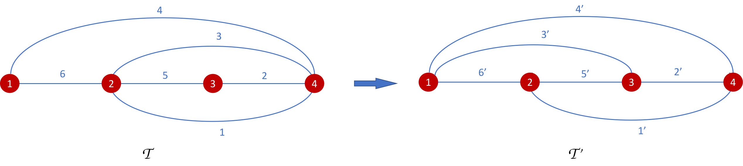
The above discussion is based on the ideal triangulation FIG.1. Changing ideal triangulation results in unitary equivalent quantization of FG coordinates. Let us denote the triangulation in FIG.1(a) by 𝒯\mathcal{T} and consider the change of triangulation from 𝒯\mathcal{T} to the tetrahedral triangulation 𝒯\mathcal{T}^{\prime} shown in FIG.2. The change is made by flipping the edge 33 in the quadrilateral bounded by edges 4,6,5,24,6,5,2. Other changes of triangulations have similar result. The edges in 𝒯\mathcal{T}^{\prime} are labelled by 1,,61^{\prime},\cdots,6^{\prime}, and their associated FG coordinates are denoted by ze=exp(Ze)z_{e}^{\prime}=\exp(Z_{e}^{\prime}), (e=1,,6e=1,\cdots,6). We may identify the triangulation and the associated data i.e. 𝒯=({e},εe1,e2)\mathcal{T}=(\{e\},\varepsilon_{e_{1},e_{2}}) and 𝒯=({e},εe1,e2)\mathcal{T}^{\prime}=(\{e^{\prime}\},\varepsilon^{\prime}_{e^{\prime}_{1},e^{\prime}_{2}}).

Classically, changing triangulation results in a change of FG coordinate. Taking 𝒯𝒯\mathcal{T}\to\mathcal{T}^{\prime} as an example, zez_{e}^{\prime} relates to zez_{e} by the following tranformation

z1\displaystyle{z}_{1}^{\prime} =\displaystyle= z1,z3=z31,\displaystyle{z}_{1},\qquad{z}_{3}^{\prime}={z}_{3}^{-1}, (6.1)
z2\displaystyle{z}_{2}^{\prime} =\displaystyle= z2(1z3),z4=1(1z31)z41,\displaystyle{z}_{2}\left(1-{z}_{3}\right),\qquad{z}_{4}^{\prime}{}^{-1}=(1-{z}_{3}^{-1}){z}_{4}^{-1}, (6.2)
z6\displaystyle{z}_{6}^{\prime} =\displaystyle= z6(1z3),z5=1(1z31)z51.\displaystyle{z}_{6}\left(1-{z}_{3}\right),\qquad{z}_{5}^{\prime}{}^{-1}=(1-{z}_{3}^{-1}){z}_{5}^{-1}. (6.3)

where we denote eae^{\prime}_{a} simply by aa. The transformation preserves the Poisson bracket in a nontrivial manner, namely we have {za,zb}=2εa,bzazb,{z~a,z~b}=2εa,bz~az~b\{z_{a}^{\prime},z_{b}^{\prime}\}={2}\varepsilon_{a,b}^{\prime}z_{a}^{\prime}z_{b}^{\prime},\ \{\tilde{z}_{a}^{\prime},\tilde{z}_{b}^{\prime}\}={2}\varepsilon_{a,b}^{\prime}\tilde{z}_{a}^{\prime}\tilde{z}_{b}^{\prime} from the Poisson bracket of za,z~az_{a},\tilde{z}_{a}, whereas εa,bεa,b\varepsilon_{a,b}\neq\varepsilon^{\prime}_{a,b}. εab\varepsilon^{\prime}_{ab} is given by

ε=(010111101110010111111001111001101110).\displaystyle\varepsilon^{\prime}=\left(\begin{array}[]{cccccc}0&-1&0&1&1&-1\\ 1&0&1&-1&-1&0\\ 0&-1&0&1&1&-1\\ -1&1&-1&0&0&1\\ -1&1&-1&0&0&1\\ 1&0&1&-1&-1&0\\ \end{array}\right). (6.10)
Refer to caption
Figure 2: Changing from the triangulation 𝒯\mathcal{T} in FIG.1(a) to the tetrahedral triangulation 𝒯\mathcal{T}^{\prime}

The quantization on 𝒯\mathcal{T} has been studied in the above. The quantization of the FG coordinates on 𝒯\mathcal{T}^{\prime} gives the quantum algebra

𝒛a𝒛b=𝐪2εab𝒛b𝒛a,𝒛~a𝒛~b=𝐪~2εab𝒛~b𝒛~a,𝒛a𝒛~b=𝒛~b𝒛a\displaystyle\bm{z}^{\prime}_{a}\bm{z}^{\prime}_{b}=\mathbf{q}^{2\varepsilon^{\prime}_{ab}}\bm{z}^{\prime}_{b}\bm{z}^{\prime}_{a},\qquad\tilde{\bm{z}}^{\prime}_{a}\tilde{\bm{z}}^{\prime}_{b}=\tilde{\mathbf{q}}^{2\varepsilon^{\prime}_{ab}}\tilde{\bm{z}}^{\prime}_{b}\tilde{\bm{z}}^{\prime}_{a},\qquad\bm{z}^{\prime}_{a}\tilde{\bm{z}}^{\prime}_{b}=\tilde{\bm{z}}^{\prime}_{b}\bm{z}^{\prime}_{a} (6.11)

The representation of this algebra relates to the representation of (4.1) (of 𝒯\mathcal{T}) by a unitary transformation known as the quantum cluster transformation, generalizing the results in [23, 5]. Firstly, we define the map i3i_{3} acting on the logarithmic coordinate

i3:𝒁a{𝒁3+2πi,a=3𝒁a+Max({εa,3,0})(𝒁3iπ),a3,\displaystyle i_{3}:\ \bm{Z}_{a}\mapsto\begin{cases}-\bm{Z}_{3}+2\pi i,&a=3\\ \bm{Z}_{a}+\mathrm{Max}(\{\varepsilon_{a,3},0\})(\bm{Z}_{3}-i\pi),&a\neq 3\end{cases}, (6.12)

or explicitly,

i3(𝒁1)\displaystyle i_{3}\left(\bm{Z}_{1}\right) =\displaystyle= 𝑿+iπ,i3(𝒁2)2L3+2𝒀+iπ,\displaystyle-\bm{X}+i\pi,\qquad i_{3}\left(\bm{Z}_{2}\right)\to-2L_{3}+2\bm{Y}+i\pi,
i3(𝒁3)\displaystyle i_{3}\left(\bm{Z}_{3}\right) =\displaystyle= L1+L2L3L4𝑿+iπ,\displaystyle-L_{1}+L_{2}-L_{3}-L_{4}-\bm{X}+i\pi,
i3(𝒁4)\displaystyle i_{3}\left(\bm{Z}_{4}\right) =\displaystyle= 2L3+2L4+𝑿2𝒀+iπ,i3(𝒁5)=L1L2+L3+L4+𝑿2𝒀+iπ,\displaystyle 2L_{3}+2L_{4}+\bm{X}-2\bm{Y}+i\pi,\qquad i_{3}\left(\bm{Z}_{5}\right)=L_{1}-L_{2}+L_{3}+L_{4}+\bm{X}-2\bm{Y}+i\pi,
i3(𝒁6)\displaystyle i_{3}\left(\bm{Z}_{6}\right) =\displaystyle= L1L2L3L42𝒀+iπ\displaystyle-L_{1}-L_{2}-L_{3}-L_{4}-2\bm{Y}+i\pi (6.13)

and the same for 𝒁~a\tilde{\bm{Z}}_{a}. They satisfy

i3(Z3)+i3(Z4)+i3(Z6)3πi=2L1,i3(Z1)+i3(Z5)+i3(Z6)3πi=2L2,\displaystyle i_{3}\left(Z_{3}\right)+i_{3}\left(Z_{4}\right)+i_{3}\left(Z_{6}\right)-3\pi i=-2L_{1},\qquad i_{3}\left(Z_{1}\right)+i_{3}\left(Z_{5}\right)+i_{3}\left(Z_{6}\right)-3\pi i=-2L_{2}, (6.14)
i3(Z2)+i3(Z3)+i3(Z5)3πi=2L3,i3(Z1)+i3(Z2)+i3(Z4)3πi=2L4\displaystyle i_{3}\left(Z_{2}\right)+i_{3}\left(Z_{3}\right)+i_{3}\left(Z_{5}\right)-3\pi i=-2L_{3},\qquad i_{3}\left(Z_{1}\right)+i_{3}\left(Z_{2}\right)+i_{3}\left(Z_{4}\right)-3\pi i=2L_{4} (6.15)

i3i_{3} induces the monomial transformation of 𝒛a\bm{z}_{a}.

i3(𝒛1)\displaystyle i_{3}\left(\bm{z}_{1}\right) =\displaystyle= 𝒙1,i3(𝒛2)=λ32𝒚2,i3(𝒛3)=λ11λ2λ31λ41𝒙1,\displaystyle-\bm{x}^{-1},\qquad i_{3}\left(\bm{z}_{2}\right)=-{\lambda_{3}^{-2}}\bm{y}^{2},\qquad i_{3}\left(\bm{z}_{3}\right)=-\lambda_{1}^{-1}\lambda_{2}\lambda_{3}^{-1}\lambda_{4}^{-1}\bm{x}^{-1},
i3(𝒛4)\displaystyle i_{3}\left(\bm{z}_{4}\right) =\displaystyle= 𝐪λ32λ42𝒙𝒚2,i3(𝒛5)=𝐪λ21λ1λ3λ4𝒙𝒚2,i3(𝒛6)=(λ1λ2λ3λ4)1𝒚2.\displaystyle-\mathbf{q}{\lambda_{3}^{2}\lambda_{4}^{2}}\bm{x}\bm{y}^{-2},\qquad i_{3}\left(\bm{z}_{5}\right)=-\mathbf{q}\lambda_{2}^{-1}\lambda_{1}\lambda_{3}\lambda_{4}\bm{x}\bm{y}^{-2},\qquad i_{3}\left(\bm{z}_{6}\right)=-{(\lambda_{1}\lambda_{2}\lambda_{3}\lambda_{4})^{-1}}\bm{y}^{2}. (6.16)

The image of i3i_{3} gives operators on \mathcal{H} with the following commutation relation

[i3(𝒁a),i3(𝒁b)]=2εab,[i3(𝒁~a),i3(𝒁~b)]=2~εab.\displaystyle\left[i_{3}(\bm{Z}_{a}),i_{3}(\bm{Z}_{b})\right]=2\hbar\varepsilon^{\prime}_{ab},\qquad\left[i_{3}(\tilde{\bm{Z}}_{a}),i_{3}(\tilde{\bm{Z}}_{b})\right]=2\tilde{\hbar}\varepsilon^{\prime}_{ab}. (6.17)

Therefore, the set of i3(𝒛a)i_{3}(\bm{z}_{a}), i3(𝒛~a)i_{3}(\tilde{\bm{z}}_{a}) satisfies the same operator algebra as (6.11). Then we define the unitary transformation

φ(𝒛3,𝒛~3):\displaystyle\varphi(-\bm{z}_{3},-\tilde{\bm{z}}_{3}):\ \mathcal{H}\to\mathcal{H}^{\prime} (6.18)

where \mathcal{H}^{\prime} carries the representation of (6.11). Both \mathcal{H} and \mathcal{H}^{\prime} as Hilbert spaces are isomorphic to L2()kL^{2}(\mathbb{R})\otimes\mathbb{C}^{k}. φ\varphi is the quantum dilogarithm and 𝒛3=λ1λ3λ4λ2𝒙\bm{z}_{3}=-\frac{\lambda_{1}\lambda_{3}\lambda_{4}}{\lambda_{2}}\bm{x}. Explicitly, for any state ff\in\mathcal{H}, ff can be represented as f~(ν,n)\widetilde{f}(\nu,n) as the Fourier transform of f(μ,ν)f(\mu,\nu). 𝒙\bm{x} acts on f~(ν,n)\widetilde{f}(\nu,n) as the multiplication of x=exp[2πik(ibνn)]x=\exp[\frac{2\pi i}{k}(-ib\nu-n)]. Then

φ(𝒛3,𝒛~3)f~(ν,n)=φ(λ1λ3λ4λ2x,λ~1λ~3λ~4λ~2x~)f~(ν,n)\displaystyle\varphi(-\bm{z}_{3},-\tilde{\bm{z}}_{3})\widetilde{f}(\nu,n)=\varphi\left(\frac{\lambda_{1}\lambda_{3}\lambda_{4}}{\lambda_{2}}x,\frac{\tilde{\lambda}_{1}\tilde{\lambda}_{3}\tilde{\lambda}_{4}}{\tilde{\lambda}_{2}}\tilde{x}\right)\widetilde{f}(\nu,n) (6.19)

Then the representation of 𝒛a,𝒛~a\bm{z}^{\prime}_{a},\tilde{\bm{z}}_{a}^{\prime} is given by

𝒛a=φ(𝒛3,𝒛~3)i3(𝒛a)φ(𝒛3,𝒛~3)1,𝒛~a=φ(𝒛3,𝒛~3)i3(𝒛~a)φ(𝒛3,𝒛~3)1.\displaystyle\bm{z}^{\prime}_{a}=\varphi(-\bm{z}_{3},-\tilde{\bm{z}}_{3})i_{3}(\bm{z}_{a})\varphi(-\bm{z}_{3},-\tilde{\bm{z}}_{3})^{-1},\qquad\tilde{\bm{z}}^{\prime}_{a}=\varphi(-\bm{z}_{3},-\tilde{\bm{z}}_{3})i_{3}(\tilde{\bm{z}}_{a})\varphi(-\bm{z}_{3},-\tilde{\bm{z}}_{3})^{-1}. (6.20)

We may compute (6.20) explicitly

𝒛1\displaystyle\bm{z}_{1}^{\prime} =\displaystyle= 𝒛1,𝒛3=𝒛31,\displaystyle\bm{z}_{1},\qquad\bm{z}_{3}^{\prime}=\bm{z}_{3}^{-1},
𝒛2\displaystyle\bm{z}_{2}^{\prime} =\displaystyle= 𝒛2(1𝐪𝒛3),𝒛4=1(1𝐪𝒛31)𝒛41,\displaystyle\bm{z}_{2}\left(1-\mathbf{q}\bm{z}_{3}\right),\qquad\bm{z}_{4}^{\prime}{}^{-1}=(1-\mathbf{q}\bm{z}_{3}^{-1})\bm{z}_{4}^{-1},
𝒛6\displaystyle\bm{z}_{6}^{\prime} =\displaystyle= 𝒛6(1𝐪𝒛3),𝒛5=1(1𝐪𝒛31)𝒛51,\displaystyle\bm{z}_{6}\left(1-\mathbf{q}\bm{z}_{3}\right),\qquad\bm{z}_{5}^{\prime}{}^{-1}=(1-\mathbf{q}\bm{z}_{3}^{-1})\bm{z}_{5}^{-1}, (6.21)

and similar for 𝒛~a\tilde{\bm{z}}^{\prime}_{a}. As 𝐪1\mathbf{q}\to 1, these transformations reduce to the classical transformation of FG coordinate under the flip.

If we denote by VsV_{s} the unitary transformation from \mathcal{H} to the direct integral representation in (5.59) for the S-cycle trace, the composition Vsϕ(𝒛3,𝒛~3)1V_{s}\circ\phi(-\bm{z}_{3},-\tilde{\bm{z}}_{3})^{-1} maps from \mathcal{H}^{\prime} to the direct integral representation.

Acknowledgements

M.H. acknowledges Chen-Hung Hsiao and Qiaoyin Pan for helpful discussions. M.H. receives supports from the National Science Foundation through grant PHY-2207763 and the College of Science Research Fellowship at Florida Atlantic University. M.H. also receives support from the visiting professorship at FAU Erlangen-Nürnberg at the early stage of this work.

Appendix A Quantum dilogarithm

The quantum dilogarithm function is defined by

φ(y,y~)\displaystyle\varphi\left(y,\tilde{y}\right) φ𝐪,𝐪~(y,y~)=[j=01+𝐪2j+1y1+𝐪~2j1y~]1ϕ(μ,m)\displaystyle\equiv\varphi_{\bf{q},\tilde{\bf q}}\left(y,\tilde{y}\right)=\left[\prod_{j=0}^{\infty}\frac{1+\mathbf{q}^{2j+1}y}{1+\tilde{\mathbf{q}}^{-2j-1}\tilde{y}}\right]^{-1}\equiv\phi(\mu,m) (A.1)

where y=exp[2πik(ibμm)]y=\exp[\frac{2\pi i}{k}(-ib\mu-m)] and y~=exp[2πik(ib1μ+m)]\tilde{y}=\exp[\frac{2\pi i}{k}(-ib^{-1}\mu+m)]. The quantum dilogarithm function satisfies the following recursion relations:

φ(𝐪2y,y~)=(1+𝐪y)φ(y,y~),φ(y,𝐪~2y~)=(1+𝐪~y~)φ(y,y~),\displaystyle\varphi\left(\mathbf{q}^{2}y,\tilde{y}\right)=\left(1+\mathbf{q}y\right)\varphi\left(y,\tilde{y}\right),\qquad\varphi\left(y,\tilde{\mathbf{q}}^{2}\tilde{y}\right)=\left(1+\tilde{\mathbf{q}}\tilde{y}\right)\varphi\left(y,\tilde{y}\right), (A.2)
φ(𝐪y,y~)=(1+y)φ(𝐪1y,y~),φ(y,𝐪~y~)=(1+y~)φ(y,𝐪~1y~),\displaystyle\varphi\left(\mathbf{q}y,\tilde{y}\right)=\left(1+y\right)\varphi\left(\mathbf{q}^{-1}y,\tilde{y}\right),\qquad\varphi\left(y,\tilde{\mathbf{q}}\tilde{y}\right)=\left(1+\tilde{y}\right)\varphi\left(y,\tilde{\mathbf{q}}^{-1}\tilde{y}\right), (A.3)
φ(y,y~)=(1+𝐪1y)φ(𝐪2y,y~),φ(y,y~)=(1+𝐪~1y~)φ(y,𝐪~2y~).\displaystyle\varphi\left(y,\tilde{y}\right)=\left(1+\mathbf{q}^{-1}y\right)\varphi\left(\mathbf{q}^{-2}y,\tilde{y}\right),\qquad\varphi\left(y,\tilde{y}\right)=\left(1+\tilde{\mathbf{q}}^{-1}\tilde{y}\right)\varphi\left(y,\tilde{\mathbf{q}}^{-2}\tilde{y}\right). (A.4)

We also use an alternative convention of the quantum dilogarithm

𝒟b(x,n)=(χ+(x+Cbk,n);𝔮2𝒘)(χ(xCbk,n);𝔮~2𝒘¯),\mathcal{D}_{b}(x,n)=\frac{\left(\chi^{+}\left(x+\frac{C_{b}}{\sqrt{k}},n\right);\mathfrak{q}^{2}\bm{w}\right)_{\infty}}{\left(\chi^{-}\left(x-\frac{C_{b}}{\sqrt{k}},n\right);\tilde{\mathfrak{q}}^{2}\bar{\bm{w}}\right)_{\infty}},

where

𝔮=e2iπb2/k,𝔮~=e2iπb2/k,𝒘=e4πi/k,Cb=i(b+b1)=2cb\displaystyle\mathfrak{q}=e^{2i\pi b^{2}/k},\qquad\tilde{\mathfrak{q}}=e^{-2i\pi b^{-2}/k},\qquad\bm{w}=e^{4\pi i/k},\qquad C_{b}={i}\left(b+b^{-1}\right)=2c_{b}
χ±(x,n)=exp[2πik(ib±1xk±n)]\displaystyle\chi^{\pm}(x,n)=\exp\left[\frac{2\pi i}{k}\left(-ib^{\pm 1}x\sqrt{k}\pm n\right)\right] (A.5)

and we have 𝔮2𝒘=e4iπ(b2+1)/k=𝐪2\mathfrak{q}^{2}\bm{w}=e^{4i\pi\left(b^{2}+1\right)/k}=\mathbf{q}^{2} and 𝔮~2𝒘¯=e4iπ(b2+1)/k=𝐪~2\mathfrak{\tilde{q}}^{2}\bar{\bm{w}}=e^{-4i\pi\left(b^{-2}+1\right)/k}=\tilde{\mathbf{q}}^{-2}. Our convention of qq-Pochammer symbol is (x;q)=j=0(1qjx)(x;q)_{\infty}=\prod_{j=0}^{\infty}\left(1-q^{j}x\right). So

𝒟b(x,n)=j=01𝐪2j+1exp[2πik(ibxk+n)]1𝐪~2j1exp[2πik(ib1xkn)]\displaystyle\mathcal{D}_{b}(x,n)=\prod_{j=0}^{\infty}\frac{1-{\bf q}^{2j+1}\exp\left[\frac{2\pi i}{k}\left(-ibx\sqrt{k}+n\right)\right]}{1-\tilde{{\bf q}}^{-2j-1}\exp\left[\frac{2\pi i}{k}\left(-ib^{-1}x\sqrt{k}-n\right)\right]} (A.6)

relates to φ(y,y~)\varphi(y,\tilde{y}) by

φ(y,y~)=𝒟b(μk,m)1\displaystyle\varphi\left(-y,-\tilde{y}\right)=\mathcal{D}_{b}\left(\frac{\mu}{\sqrt{k}},-m\right)^{-1} (A.7)

When k=2Nk=2N is even (NN\in\mathbb{Z}), the quantum dilogarithm Db(x,n){\rm D}_{b}(x,n) used in [10, 11] is related by

Db(x,n)=𝒟b(2x,2n),φ(y2,y~2)=Db(μN,m)1.\displaystyle{\rm D}_{b}(x,n)=\mathcal{D}_{b}(\sqrt{2}x,2n),\qquad\varphi\left(-y^{2},-\tilde{y}^{2}\right)={\rm D}_{b}\left(\frac{\mu}{\sqrt{N}},-m\right)^{-1}. (A.8)

We also introduce 131313This notation is inspired by [7].

γ(x,n)=Db(x,n).\displaystyle\gamma(x,n)=\mathrm{D}_{b}(-x,n). (A.9)

The quantum dilogarithm functions satisfy the unitarity

ϕ(μ,m)=ϕ(μ,m)1,𝒟b(x,n)=𝒟b(x,n)1,γ(x,n)=γ(x,n)1.\displaystyle\phi\left(\mu,m\right)^{*}=\phi\left(\mu^{*},m\right)^{-1},\qquad\mathcal{D}_{b}(x,n)^{*}=\mathcal{D}_{b}(x^{*},n)^{-1},\qquad\gamma(x,n)^{*}=\gamma(x^{*},n)^{-1}. (A.10)

We introduce some notations ω,ω,ω′′\omega,\omega^{\prime},\omega^{\prime\prime} by

ω=i2bN,ω=ib2N,ω′′=cbN.\displaystyle\omega=\frac{i}{2b\sqrt{N}},\quad\omega^{\prime}=\frac{ib}{2\sqrt{N}},\quad\omega^{\prime\prime}=\frac{c_{b}}{\sqrt{N}}\ . (A.11)

The following summarizes some useful properties of γ(x,n)\gamma(x,n):

  • The inverse relation:

    γ(x,n)γ(x,n)=exp(iπn2NiπniπN6+iπx213iπω′′)2.\displaystyle\gamma(x,n)\gamma(-x,-n)=\exp\left(-\frac{i\pi n^{2}}{N}-i\pi n-\frac{i\pi N}{6}+i\pi x^{2}-\frac{1}{3}i\pi\omega^{\prime\prime}{}^{2}\right). (A.12)
  • The recursion relation:

    γ(x±2ω,n1)\displaystyle\gamma(x\pm 2\omega^{\prime},n\mp 1) =\displaystyle= (1+e2iπnN±iπ(N1)N+4iπxω±4iπω2)±1γ(x,n),\displaystyle\left(1+e^{\frac{2i\pi n}{N}\pm\frac{i\pi(N-1)}{N}+4i\pi x\omega^{\prime}\pm 4i\pi\omega^{\prime}{}^{2}}\right)^{\pm 1}\gamma(x,n), (A.13)
    γ(x±2ω,n±1)\displaystyle\gamma(x\pm 2\omega,n\pm 1) =\displaystyle= (1+e2iπnN±iπ(N1)N+4iπxω±4iπω2)±1γ(x,n).\displaystyle\left(1+e^{-\frac{2i\pi n}{N}\pm\frac{i\pi(N-1)}{N}+4i\pi x\omega\pm 4i\pi\omega^{2}}\right)^{\pm 1}\gamma(x,n). (A.14)
  • The integration identity:

    1Nd/Ndtγ(t+α,a+d)γ(t+β,p+d)e2iπste2iπcdN\displaystyle\frac{1}{\sqrt{N}}\sum_{d\in\mathbb{Z}/N\mathbb{Z}}\int\mathrm{d}t\frac{\gamma(t+\alpha,a+d)}{\gamma(t+\beta,p+d)}e^{-2i\pi st}e^{-\frac{2i\pi cd}{N}} (A.15)
    =\displaystyle= ζ0e2iπacN+2iπs(α+ω′′)γ(α+β+sω′′,ac+p)γ(s+ω′′,c)γ(α+βω′′,pa),\displaystyle\zeta_{0}\,e^{\frac{2i\pi ac}{N}+2i\pi s\left(\alpha+\omega^{\prime\prime}\right)}\frac{\gamma\left(-\alpha+\beta+s-\omega^{\prime\prime},-a-c+p\right)}{\gamma\left(s+\omega^{\prime\prime},-c\right)\gamma\left(-\alpha+\beta-\omega^{\prime\prime},p-a\right)},

    where ζ0=e112iπ(N4cb2N)\zeta_{0}=e^{-\frac{1}{12}i\pi\left(N-\frac{4c_{b}^{2}}{N}\right)} and α,β,s\alpha,\beta,s satisfy

    Im(α+cbN)>0,Im(β+cbN)>0,Im(αβ)<Im(s)<0.\displaystyle\mathrm{Im}(\alpha+\frac{c_{b}}{\sqrt{N}})>0,\qquad\mathrm{Im}(-\beta+\frac{c_{b}}{\sqrt{N}})>0,\qquad\mathrm{Im}(\alpha-\beta)<\mathrm{Im}(s)<0. (A.16)

    The inverse of the identity:

    γ(α+t,a+d)γ(β+t,d+p)\displaystyle\frac{\gamma(\alpha+t,a+d)}{\gamma(\beta+t,d+p)} (A.17)
    =\displaystyle= ζ0Nc/Ndsγ(α+β+sω′′,ac+p)e2iπ(a+d)cN+2iπs(α+ω′′)+2iπstγ(s+ω′′,c)γ(α+βω′′,pa).\displaystyle\frac{\zeta_{0}}{\sqrt{N}}\sum_{c\in\mathbb{Z}/N\mathbb{Z}}\int\mathrm{d}s\frac{\gamma\left(-\alpha+\beta+s-\omega^{\prime\prime},-a-c+p\right)e^{\frac{2i\pi(a+d)c}{N}+2i\pi s\left(\alpha+\omega^{\prime\prime}\right)+2i\pi st}}{\gamma\left(s+\omega^{\prime\prime},-c\right)\gamma\left(-\alpha+\beta-\omega^{\prime\prime},p-a\right)}.

Appendix B Fock-Goncharov coordinate and holonomies
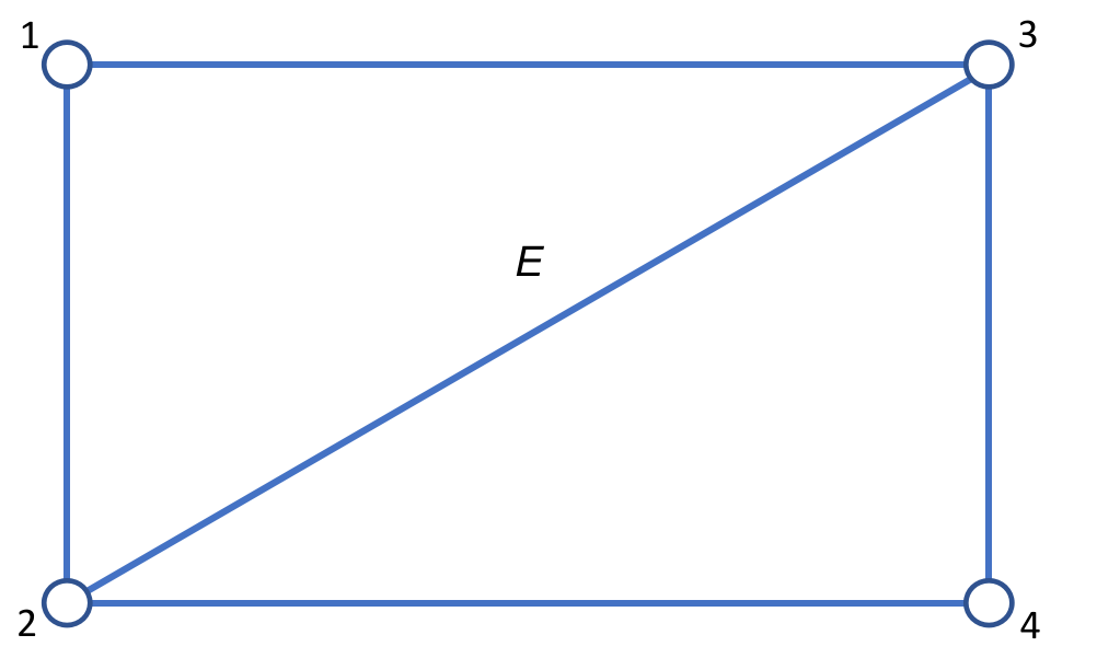
Refer to caption
Figure 3:

A 2-sphere in which nn discs are removed is a nn-holed sphere. We make a 2d ideal triangulation of the nn-holed sphere such that edges in the triangulation end at the boundary of the holes. For example, the boundary of the ideal tetrahedron is an ideal triangulation of the 4-holed sphere. The 2d ideal triangulation has 3(n2)3(n-2) edges on the nn-holed sphere. Each edge EE associates to a coordinate zEz_{E} of the moduli space of framed SL(2,)\mathrm{SL}(2,\mathbb{C}) flat connections. A framed flat connection on is a standard flat connection with a choice of 1\mathbb{CP}^{1} flat section sis_{i} for each hole ii. The section sis_{i} obeying the condition si=0\nabla s_{i}=0 (\nabla is the flat connection) and is the eigenvector of monodromy around the hole ii. sis_{i} associates to the eigenvalue λi=eLi\lambda_{i}=e^{L_{i}} of the monodromy matrix. Given a framed flat connection, zEz_{E} is a cross-ratio of 4 flat section s1,s2,s3,s4s_{1},s_{2},s_{3},s_{4} associated to the vertices of the quadrilateral containing EE as the diagonal (see FIG.3),

zE=s1s2s3s4s1s3s2s4\displaystyle z_{E}=\frac{\left\langle s_{1}\wedge s_{2}\right\rangle\left\langle s_{3}\wedge s_{4}\right\rangle}{\left\langle s_{1}\wedge s_{3}\right\rangle\left\langle s_{2}\wedge s_{4}\right\rangle} (B.1)

where sisj\left\langle s_{i}\wedge s_{j}\right\rangle is an SL(2,)\mathrm{SL}(2,\mathbb{C}) invariant volume on 2\mathbb{C}^{2}, and is computed by parallel transporting s1,,s4s_{1},\cdots,s_{4} to a common point inside the quadrilateral by the flat connection. The coordinates zEz_{E} for all EE are the Fock-Goncharov (FG) coordinates. Our convention is the same as [24, 9]. We often consider a lift of zEz_{E} to the logarithmic coordinate ZEZ_{E} such that zE=eZEz_{E}=e^{Z_{E}}. At any hole ii, zEz_{E} on the adjacent edges EE satisfy

Eati(zE)=λi2.\displaystyle\prod_{E\ \text{at}\ i}(-z_{E})=\lambda_{i}^{2}. (B.2)

We often use the lift of this relation

Eati(ZEπi)=2Li.\displaystyle\sum_{E\ \text{at}\ i}(Z_{E}-\pi i)=2L_{i}. (B.3)

Note that L1,,3L_{1,\cdots,3} in (4.10) are defined with flipped sign.

SL(2,)\mathrm{SL}(2,\mathbb{C}) holonomy along any closed path on the nn-holed sphere can be expressed as 2×22\times 2 matrices whose entries are functions of {ZE}\{Z_{E}\} by using the “snake rule” [22]: There are three rules for transporting a snake – an arrow pointing from one vertex of the triangle to another with a fin facing inside the triangle, each corresponds to a matrix as follows. (The inverse transportation of each type corresponds to the inverse of the relevant matrix.

[Uncaptioned image][Uncaptioned image][Uncaptioned image].\displaystyle\includegraphics[width=110.57327pt]{snake_rule1.pdf}\quad\qquad\includegraphics[width=110.57327pt]{snake_rule2.pdf}\quad\qquad\includegraphics[width=132.68929pt]{snake_rule3}\,. (B.4)

A snake represents a projective basis (v1,v2)(v_{1},v_{2}) given by v1v_{1}\in\mathbb{C} at the tail of the snake and v2v_{2}\in\mathbb{C} at the head of the snake, such that either v1+v2v_{1}+v_{2} (type I: blue) or v1v2v_{1}-v_{2} (type I: red) at the third vertex of the triangle. Type I and II correspond to transporting a snake within a triangle and III correspond to moving a snake from one triangle to its adjacent triangle. The transformation matrix acts on the projective basis (v1,v2)T(v_{1},v_{2})^{T} by left multiplication. Any holonomy H(γ)H(\gamma) of a closed loop γ\gamma can be calculated by multiplying the matrices from right to left corresponding to moving a snake along the loop. The holonomy resulting from the snake rule is not SL(2,)\mathrm{SL}(2,\mathbb{C}). The SL(2,)\mathrm{SL}(2,\mathbb{C}) holonomy is obtained up to a ±\pm sign by a lift that can conveniently chosen by normalizing the Type III matrix

Type III:(eZEπi200eZEπi2)E[ZE].\displaystyle\text{Type III:}\qquad\left(\begin{array}[]{cc}e^{-\frac{Z_{E}-\pi i}{2}}&0\\ 0&e^{\frac{Z_{E}-\pi i}{2}}\end{array}\right)\equiv E[Z_{E}]. (B.7)

For any closed path γi\gamma_{i} around a single hole ii, the ±\pm sign of H(γi)H(\gamma_{i}) can be determined by requiring the trace of H(γi)H(\gamma_{i}) to be

Tr(H(γi))=e12Eati(ZEiπ)+e12Eati(ZEiπ)=eLi+eLi.\displaystyle\mathrm{Tr}(H(\gamma_{i}))=e^{\frac{1}{2}\sum_{E\ \text{at}\ i}(Z_{E}-i\pi)}+e^{-\frac{1}{2}\sum_{E\ \text{at}\ i}(Z_{E}-i\pi)}=e^{L_{i}}+e^{-L_{i}}. (B.8)

This requirements is consistent with (B.3) and the eigenvalue of the monodromy matrix when discussing sis_{i}. The fundamental group of the nn-holed sphere is generated by {γi}i=1,,n\{\gamma_{i}\}_{i=1,\dots,n}, so {H(γi)}i=1,,n\{H(\gamma_{i})\}_{i=1,\dots,n} determine all holonomies of closed paths.

Refer to caption
Figure 4: The tetrahedral ideal triangulation of 4-holed sphere and the FG coordinates z,z,z′′z,z^{\prime},z^{\prime\prime}.

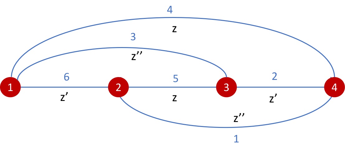
We consider the 4-holed sphere and the ideal triangulation in FIG.4 as an example. The ideal triangulation is tetrahedral since it is the boundary of an ideal tetrahedron. We denote by γi\gamma_{i} a loop around the hole ii oriented counter-clockwisely. All γi\gamma_{i} share the same base point represented by a snake pointing from the 4th hole to the 2nd hole along the edge 1 with the fin inside the triangle with vertices 2,3,42,3,4.

H(γ4)\displaystyle H(\gamma_{4}) =\displaystyle= (1011)E(Z2)(1011)E(Z4)(1011)E(Z1),\displaystyle\left(\begin{array}[]{cc}1&0\\ 1&1\\ \end{array}\right)E\left(Z_{2}\right)\left(\begin{array}[]{cc}1&0\\ 1&1\\ \end{array}\right)E\left(Z_{4}\right)\left(\begin{array}[]{cc}1&0\\ 1&1\\ \end{array}\right)E\left(Z_{1}\right), (B.15)
H(γ3)\displaystyle H(\gamma_{3}) =\displaystyle= (0110)(1011)1(0110)E(Z5)(1011)E(Z3)(1011)(0110)1E(Z2)1(1011)1,\displaystyle-\left(\begin{array}[]{cc}0&1\\ -1&0\\ \end{array}\right)\left(\begin{array}[]{cc}1&0\\ 1&1\\ \end{array}\right)^{-1}\left(\begin{array}[]{cc}0&1\\ -1&0\\ \end{array}\right)E\left(Z_{5}\right)\left(\begin{array}[]{cc}1&0\\ 1&1\\ \end{array}\right)E\left(Z_{3}\right)\left(\begin{array}[]{cc}1&0\\ 1&1\\ \end{array}\right)\left(\begin{array}[]{cc}0&1\\ -1&0\\ \end{array}\right)^{-1}E\left(Z_{2}\right)^{-1}\left(\begin{array}[]{cc}1&0\\ 1&1\\ \end{array}\right)^{-1}, (B.30)
H(γ2)\displaystyle H(\gamma_{2}) =\displaystyle= (0110)E(Z1)(1011)E(Z6)(1011)E(Z5)(1011)(0110)1,\displaystyle\left(\begin{array}[]{cc}0&1\\ -1&0\\ \end{array}\right)E\left(Z_{1}\right)\left(\begin{array}[]{cc}1&0\\ 1&1\\ \end{array}\right)E\left(Z_{6}\right)\left(\begin{array}[]{cc}1&0\\ 1&1\\ \end{array}\right)E\left(Z_{5}\right)\left(\begin{array}[]{cc}1&0\\ 1&1\\ \end{array}\right)\left(\begin{array}[]{cc}0&1\\ -1&0\\ \end{array}\right)^{-1}, (B.41)
H(γ4)\displaystyle H(\gamma_{4}) =\displaystyle= (0110)E(Z1)(1011)(0110)1(1011)E(Z4)(1011)E(Z3)(1011)E(Z6)\displaystyle\left(\begin{array}[]{cc}0&1\\ -1&0\\ \end{array}\right)E\left(Z_{1}\right)\left(\begin{array}[]{cc}1&0\\ 1&1\\ \end{array}\right)\left(\begin{array}[]{cc}0&1\\ -1&0\\ \end{array}\right)^{-1}\left(\begin{array}[]{cc}1&0\\ 1&1\\ \end{array}\right)E\left(Z_{4}\right)\left(\begin{array}[]{cc}1&0\\ 1&1\\ \end{array}\right)E\left(Z_{3}\right)\left(\begin{array}[]{cc}1&0\\ 1&1\\ \end{array}\right)E\left(Z_{6}\right) (B.61)
(0110)(1011)1E(Z1)(0110)11.\displaystyle\left(\begin{array}[]{cc}0&1\\ -1&0\\ \end{array}\right)\left(\begin{array}[]{cc}1&0\\ 1&1\\ \end{array}\right)^{-1}E\left(Z_{1}\right){}^{-1}\left(\begin{array}[]{cc}0&1\\ -1&0\\ \end{array}\right)^{-1}.

They satisfy Tr(H(γi))=eLi+eLi\mathrm{Tr}(H(\gamma_{i}))=e^{L_{i}}+e^{-L_{i}} and

H(γ1)H(γ2)H(γ3)H(γ4)=1.\displaystyle H(\gamma_{1})H(\gamma_{2})H(\gamma_{3})H(\gamma_{4})=1. (B.62)

When the 4-holed sphere is the boundary of an ideal tetrahedron, all H(γi)H(\gamma_{i}) are constrained to the identity matrix, since the connection is flat inside the tetrahedron. In this case, all LiL_{i} vanishes, i.e.

Z1+Z2+Z4=Z3+Z4+Z6=Z1+Z5+Z6=Z2+Z3+Z5=3πi\displaystyle Z_{1}+Z_{2}+Z_{4}=Z_{3}+Z_{4}+Z_{6}=Z_{1}+Z_{5}+Z_{6}=Z_{2}+Z_{3}+Z_{5}=3\pi i (B.63)

so we can parametrize zez_{e} by calling the FG coordinates z,z,z′′z,z^{\prime},z^{\prime\prime} occurring in the same counter-clockwise order around any hole, equal on opposite edges, and satisfying 141414We relabel z1=z3=z′′,z2=z6=z,z4=z5=zz_{1}=z_{3}=z^{\prime\prime},\ z_{2}=z_{6}=z^{\prime},\ z_{4}=z_{5}=z.

zzz′′=1.\displaystyle zz^{\prime}z^{\prime\prime}=-1. (B.64)

The off-diagonal vanishes implies

z′′+z11=0.\displaystyle z^{\prime\prime}+z^{-1}-1=0. (B.65)

z,z′′z,z^{\prime\prime} are the symplectic coordinates of the phase space (of flat connections) on the boundary of ideal tetrahedron, with the poisson bracket given by {Z′′,Z}={Z,Z}={Z,Z′′}=2\{Z^{\prime\prime},Z\}=\{Z,Z^{\prime}\}=\{Z^{\prime},Z^{\prime\prime}\}=2. Eq.(B.65) defines the Lagrangian submanifold Δ\mathcal{L}_{\Delta} of the flat connections that can be extended to interior of the tetrahedron.

References

  • [1] R. M. Kashaev, On the spectrum of Dehn twists in quantum Teichmuller theory, math/0008148.
  • [2] A. G. Bytsko and J. Teschner, R operator, coproduct and Haar measure for the modular double of U(q)(sl(2,R)), Commun. Math. Phys. 240 (2003) 171–196, [math/0208191].
  • [3] I. Nidaiev and J. Teschner, On the relation between the modular double of Uq(sl(2,R))U_{q}(sl(2,R)) and the quantum Teichmueller theory, arXiv:1302.3454.
  • [4] B. Ponsot and J. Teschner, Clebsch-Gordan and Racah-Wigner coefficients for a continuous series of representations of U(q)(sl(2,R)), Commun. Math. Phys. 224 (2001) 613–655, [math/0007097].
  • [5] J. Teschner, An Analog of a modular functor from quantized teichmuller theory, math/0510174.
  • [6] J. Teschner, On the relation between quantum Liouville theory and the quantized Teichmuller spaces, Int. J. Mod. Phys. A 19S2 (2004) 459–477, [hep-th/0303149].
  • [7] S. E. Derkachov and L. D. Faddeev, 3j-symbol for the modular double of SLq(2,)SL_{q}(2,\mathbb{R}) revisited, J. Phys. Conf. Ser. 532 (2014) 012005, [arXiv:1302.5400].
  • [8] T. P. Killingback, Quantization of SL(2,R) Chern-Simons theory, Commun. Math. Phys. 145 (1992) 1–16.
  • [9] J. Teschner, Supersymmetric gauge theories, quantisation of moduli spaces of flat connections, and Liouville theory, arXiv:1412.7140.
  • [10] J. Ellegaard Andersen and R. Kashaev, Complex Quantum Chern-Simons, ArXiv e-prints (Sept., 2014) [arXiv:1409.1208].
  • [11] J. E. Andersen and S. Marzioni, Level n teichmüller tqft and complex chern-simons theory, arXiv:1612.06986.
  • [12] T. Dimofte, Complex Chern-Simons Theory at Level k via the 3d-3d Correspondence, Commun. Math. Phys. 339 (2015), no. 2 619–662, [arXiv:1409.0857].
  • [13] E. Witten, Quantization of chern-simons gauge theory with complex gauge group, Communications in Mathematical Physics 137 (1991), no. 1 29–66.
  • [14] A. Goncharov and L. Shen, Quantum geometry of moduli spaces of local systems and representation theory, 2022.
  • [15] P. Podleś and S. L. Woronowicz, Quantum deformation of Lorentz group, Comm. Math. Phys. 130 (1990), no. 2 381–431.
  • [16] E. Buffenoir and P. Roche, Harmonic analysis on the quantum Lorentz group, Commun.Math.Phys. 207 (1999) 499–555, [q-alg/9710022].
  • [17] E. Buffenoir, K. Noui, and P. Roche, Hamiltonian quantization of Chern-Simons theory with SL(2,C) group, Class.Quant.Grav. 19 (2002) 4953, [hep-th/0202121].
  • [18] M. Han, Four-dimensional spinfoam quantum gravity with a cosmological constant: Finiteness and semiclassical limit, Phys. Rev. D 104 (2021), no. 10 104035, [arXiv:2109.00034].
  • [19] H. M. Haggard, M. Han, W. Kaminski, and A. Riello, SL(2,C) Chern-Simons Theory, a non-Planar Graph Operator, and 4D Loop Quantum Gravity with a Cosmological Constant: Semiclassical Geometry, Nucl. Phys. B900 (2015) 1–79, [arXiv:1412.7546].
  • [20] H. M. Haggard, M. Han, W. Kaminski, and A. Riello, Four-dimensional Quantum Gravity with a Cosmological Constant from Three-dimensional Holomorphic Blocks, Phys. Lett. B752 (2016) 258–262, [arXiv:1509.00458].
  • [21] M. Han and Q. Pan, Melonic Radiative Correction in Four-Dimensional Spinfoam Model with Cosmological Constant, arXiv:2310.04537.
  • [22] T. Dimofte, D. Gaiotto, and R. van der Veen, RG Domain Walls and Hybrid Triangulations, Adv.Theor.Math.Phys. 19 (2015) 137–276, [arXiv:1304.6721].
  • [23] V. V. Fock and A. B. Goncharov, The quantum dilogarithm and representations of quantum cluster varieties, Inventiones Mathematicae 175 (Sept., 2008) 223–286, [math/0702397].
  • [24] D. Gaiotto, G. W. Moore, and A. Neitzke, Wall-crossing, Hitchin Systems, and the WKB Approximation, arXiv:0907.3987.