Rendez-vous with massive interstellar objects, as triggers of destabilisation
Abstract
We study how close passages of interstellar objects of planetary and substellar masses may affect the immediate and long-term dynamics of the Solar system. We consider two nominal approach orbits, namely, the orbits of actual interstellar objects 1I/’Oumuamua and 2I/Borisov, assuming them to be typical or representative for interstellar swarms of matter. Thus, the nominal orbits of the interloper in our models cross the inner part of the Solar system. Series of massive numerical experiments are performed, in which the interloper’s mass is varied with a small step over a broad range. We find that, even if a Jovian-mass interloper does not experience close encounters with the Solar system planets (and this holds for our nominal orbits), our planetary system can be destabilised on timescales as short as several million years. In what concerns substellar-mass interlopers (free-floating brown dwarfs), an immediate (on a timescale of –100 yr) consequence of such a MISO flyby is a sharp increase in the orbital eccentricities and inclinations of the outer planets. On an intermediate timescale (– yr after the MISO flyby), Uranus or Neptune can be ejected from the system, as a result of their mutual close encounters and encounters with Saturn. On a secular timescale (– yr after the MISO flyby), the perturbation wave formed by secular planetary interactions propagates from the outer Solar system to its inner zone.
1Saint Petersburg State University, 7/9 Universitetskaya nab., 199034 Saint Petersburg, Russia
2Institute of Applied Astronomy, Russian Academy of
Sciences, 191187 Saint Petersburg, Russia
Email: [email protected]
Keywords: celestial mechanics – planets and satellites: dynamical evolution and stability – exoplanets – ISM: individual objects: 1I/’Oumuamua – ISM: individual objects: 2I/Borisov
Introduction
A free-floating planet (FFP) is understood as an interstellar object of planetary mass; in other words, it is a planet that is not gravitationally bound to any star. According to modern estimates, in our Galaxy, the number of FFPs with Jovian and greater masses should exceed the number of main-sequence stars by at least several times (Mróz et al. 2017). Given the age and number of typical stars in the Milky Way, this means that a close encounter between a star and an FFP should not be an exotic phenomenon. Indeed, according to Goulinski & Ribak (2018), approximately of the number of stars with a mass less than two Solar masses experience a temporary capture of a FFP during their lifetime; therefore, the star fraction that experience an encounter with FFPs should be considerably higher. The study of interactions of planetary systems with such objects is of great interest, since they directly relate to the problem of stability and long-term evolution and survival of planetary systems.
The FFPs and brown dwarfs (BDs) are regarded as objects of planetary and substellar masses, respectively. The upper mass limit for a planet is 13 (Jupiter masses). With a larger mass value, deuterium ignites in the core and the planet passes into the BD category (Lecavelier des Etangs & Lissauer 2022); the upper mass limit for BD is .
In this paper, we investigate the influence of flybys of massive interstellar objects (MISOs), such as FFPs or BDs, on the immediate and long-term dynamical evolution of the Solar system.
As for higher-mass MISOs (i.e., stars), encounters with them has been already studied, mostly by numerical-analytical means, in various settings in application both to our Solar system (Malmberg et al. 2011; Li & Adams 2015; Dotti et al. 2019; Stock et al. 2020; Zink et al. 2020) and model planetary systems (Laughlin & Adams 1998; Zakamska & Tremaine 2004; Portegies Zwart & Jílková 2015; Zheng et al. 2015; Cai et al. 2017). For our Solar system, it was concluded that encounters with stars that lead to immediate destabilisation must be too rare to occur on the timescales less than tens of gigayears.111By the “destabilisation” of a planetary system we imply either immediate or time-delayed loss (caused by the interloper flyby) of any of the system’s planets. Zakamska & Tremaine (2004) and Brown & Rein (2022) considered long-term consequences of such encounters; they outlined that, due to secular perturbations among planets, the post-flyby destabilisation may reveal itself on timescales much longer than orbital ones, after millions of years elapsed.
Apart from the stellar hazard, a potentially hazardous role of less massive free-floating objects should not be underestimated. According to modern concepts (see, e. g., Taylor 1999; Morbidelli 2002, and references therein), the planets in any planetary system are formed of relatively small building blocks — planetary embryos, Mercury-sized or even Mars-sized; many of them escape from the system at its early evolution stage, when it is violently unstable. Mercury may be nothing but a last such embryo survived in the Solar system; however, it is also expected to escape on a gigayear timescale; see Laskar & Gastineau (2009), and references therein. During early stages of evolution of planetary systems, collisions of the embryos with newly-formed planets may result in forming binary rocky planets (such as the Earth–Moon system) and in occurrence of large obliquities of rotation axes of giant planets (such as that of Uranus); see Safronov (1966); Chambers et al. (1996); Chambers & Wetherill (1998); Agnor et al. (1999); Morbidelli (2002). As soon as such “post-collision” phenomena seem to be actually present in our Solar system, one may speculate that a huge number of embryos may indeed escape from evolving planetary systems and form a population of interstellar objects, apart from the large-sized FFPs that are directly observed now in various surveys. A relevant estimate of the concentration of stars in the Solar neighbourhood is pc-3 (Brown & Rein, 2022). Assuming that the stars typically possess planetary systems, the concentration of free-floating embryos, resulting from the formation processes, could be in orders of magnitude greater.
FFPs may originate not only from planetary systems with host stars, but also in interstellar space, as a result of gravitational collapse of interstellar gas blobs; Goulinski & Ribak (2018) point out that various formation mechanisms may provide the FFP concentration in the Galactic Thin Disc in the range from pc-3 to pc-3.
Certain observational constraints on the flux of interstellar objects (ISOs) in our Galactic neighbourhood exist; they can be used to estimate the flux in dependence on the ISO’s size. According to (Jewitt & Seligman, 2022, Figure 19), the flux seems to follow a object’s radius distribution. If valid, this law predicts that on average the Solar system can be crossed per year by more than a dozen interstellar objects with 1 km, and, per a billion years, by more than a dozen objects with 1000 km.
In summary, the chance of encountering an FFP or BD by the Solar system is definitely non-zero; this makes a study of consequences of such an event actual. For such a study, the choice of not only the MISO mass, but also of its orbit initial conditions, can be broad. Here, we limit ourselves to considering two nominal MISO approach trajectories. Namely, for the approach orbits we choose the hyperbolic orbits of real interstellar objects 1I/’Oumuamua and 2I/Borisov, which visited the Solar system in 2017 and 2019, respectively (Bannister et al. 2017; Bialy & Loeb 2018; Jewitt & Loo 2019); henceforth we call them orbit I and orbit II, respectively. We assume them to be typical, or representative, for interstellar swarms of matter. These orbits are specific in that they intersect the inner zone of the Solar system; see Fig. 1.
For the both approach orbits, we implement problem settings that differ only in the MISO mass. Based on the results of our integrations, we estimate the degree of influence of the MISO flyby on the immediate and long-term orbital dynamics of the Solar system.
The model set-up
The performed numerical experiments are basically of similar methodology kind. For each of the adopted approach orbits I and II, a representative set of the MISO mass values is considered; namely, the masses are taken in the ranges typical for FFPs and BDs. The total number of numerical experiments for each of the approach orbits is rather large (2000), as the mass is varied in small steps; see Table 1.
| MISO type | Mass range, | Step in mass, |
|
|
||||
|---|---|---|---|---|---|---|---|---|
| FFP | – | |||||||
| BD | – |
The gravitational interaction of the MISO with the Sun and eight major Solar system planets (from Mercury to Neptune) is considered. All ten bodies are regarded as gravitating points. Note that relativistic effects are not taken into account, since, according to Laskar & Gastineau (2009) (see also Brown & Rein 2023), they influence the Solar system stability on gigayear timescales (diminishing chances for ejection of Mercury), whereas the timescales of our simulations do not exceed 5 million years.
At the initial time moment , the MISO moves at a distance from the Sun; it approaches the Solar system along a hyperbolic heliocentric orbit. The total configuration, consisting of ten moving points, is integrated, until the MISO, after passing the perihelion of its orbit, is away from the Sun by the same “threshold” distance . The MISO is then “switched off” (removed from the integrated configuration), but the planetary system is being integrated further on. The integration is stopped when time, counted from the initial time epoch , becomes equal to a fixed large constant . The adopted values of and are given in Table 1. If any of the Solar system planets eventually escapes at a time moment less than , the integration is also stopped.
The threshold distance and the maximum integration time are determined as follows. The value of should be large enough so that the gravitational influence of the MISO on the Solar system were negligible. Varvoglis et al. (2012) and Goulinski & Ribak (2018) modeled interaction between a Jupiter-mass MISO and the Sun–Jupiter binary system, and they set the initial MISO heliocentric distance equal to sizes of the binary. Here we use a much greater (by an order of magnitude) value of : for FFP-type and BD-type MISOs we respectively set AU and 60000 AU (i.e., up to about one light-year).
In orbits I and II, it takes respectively 4 and 20 thousand years for the MISO to cover its trajectory completely from its initial point up to the point of its removal from the computation.
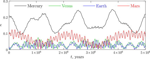
We aim to study not only the immediate but also the long-term effect of MISO flybys on the Solar system stability. To this end, it is reasonable to choose the integration time interval to be longer than, or at least similar to, the timescales of intrinsic long-term variations of orbital elements of the Solar system planets. Those were thoroughly explored and are well-known; see, e. g., Laskar (1996); Murray & Dermott (1999); Mogavero & Laskar (2021). According to Mogavero & Laskar (2021), the long-term variations of eccentricities and inclinations of the inner planets occur on the timescale of – yr; see also our Fig. 2 demonstrating this behaviour on the 5 Myr interval in the future. According to Fig. 2 in Mogavero & Laskar (2021) and Fig. 9 in Laskar (1996), the orbital eccentricity of Mars fluctuates on the timescale Myr. In our numerical experiments with planet-mass MISOs, we take to be twice this value, namely 5 Myr. For substellar-mass MISO flybys, can be more than halved, because in this case the Solar system dynamics becomes significantly unstable, as we will see further on, on a timescale as small as 1–2 Myr.
| Orbit | , AU | ,∘ | , JD | ,∘ | ,∘ | , JD | |
|---|---|---|---|---|---|---|---|
| I | |||||||
| II |
For the elements of orbit I and II we adopt those given in the NASA JPL database (accessed January 16, 2023), see Table 2. The Solar and planetary masses are taken from the same database.
We work in the heliocentric coordinate system , to which the orbital elements of the MISO and planets are assigned. First, we calculate the planetary elements for the same time for which the elements of a stellar intruder are given (see Table 2). Based on the elements and using standard algorithms (see, e. g., Herrick 1971; Battin 1999; Kholshevnikov & Titov 2007), we obtain the positions and velocities of the planets and interstellar object in the system at the time . Then, we numerically integrate this configuration backwards in time until the massless interstellar object reaches the heliocentric distance .
| Orbit | MISO type | , JD |
|
|
|---|---|---|---|---|
| I | FFP | (April 2, 135 BC) | ||
| II | FFP | (October 21, 258 AD) | ||
| I | BD | (October 11, 8750 BC) | ||
| II | BD | (August 10, 6790 BC) |
The configuration obtained in this way is considered to be the initial one corresponding to the time epoch . The interaction time interval is approximately twice as long as the time elapsed between epochs and . The values of calculated in our experiments are given in Table 3.
In the course of integration, we calculate the maximum values of the planetary eccentricities and inclinations
| (1) |
as well as quantities
| (2) | ||||
measured in AU. To calculate all 24 quantities , , a time step of 5 yr is used, and the maxima and minima in the right-hand sides of (1) and (2) are taken over the total integration interval.
We also calculate the relative deviations of the energy integral:
where and are, respectively, the initial and final values of the system total energy. The calculation of is carried out separately (1) during the preliminary backward integration, (2) during the interaction phase (beginning at and ending with the exclusion of the MISO from the system), and (3) during the further evolution of the planetary system. Since the total energies at these three stages are different, for the final energy deviation value we take the largest of these three quantities.
Integrators and computations
In all computations presented here, we use the IAS15 high-precision non-symplectic integrator implemented in the REBOUND software package (Rein & Liu, 2012; Rein & Spiegel, 2015). The universal system REBOUND, written in the general-purpose language C, contains a large set of integrators designed to model a broad range of celestial-mechanical and astrophysical problems.
In REBOUND, the equations of motion are integrated in Cartesian coordinates, which should be referred to an inertial frame of reference. To prevent a systematic drift of the bodies relative to the origin of coordinates during the simulation (if the total momentum of the system is non-zero), REBOUND can reduce the equations of motion into a barycentric reference frame before starting the integration. This feature is especially useful if the computations are performed over long time intervals.
In our computations, the astronomical system of units (Solar mass, mean Solar day, and astronomical unit) is adopted; the gravitational constant is , where the Gauss constant .
The computing resources of the Joint Supercomputer Center of the Russian Academy of Sciences (JSCC RAS, see Savin et al. 2019 and https://www.jscc.ru/) were used. Each MPI process ran one instance of REBOUND with a given value of the MISO mass. The numerical experiments typically took time from 15 to 25 hr each.
Post-flyby immediate and long-term effects
Planet-mass MISOs
Let us consider first the results obtained for planet-mass MISOs in orbit I.
The immediate (just after the flyby) eccentricities and inclinations are presented, as functions of the MISO mass, in Fig. 3 (for the inner planets) and in Fig. 4 (for the outer planets). These are the values observed at the time moment of the MISO exclusion from the system.
As follows from Figs. 3 and 4, the most prone to immediate excitation are the orbits of the outermost planets, Uranus and Neptune. For all other planets, the eccentricities and inclinations are excited much less, and they demonstrate much smaller variations with the increase of MISO’s mass.
On longer timescales, the evolved orbital parameters of the inner and outer planets are illustrated, respectively, in Figs. 5 and 6. Namely, the graphs show, as functions of the MISO mass, the maximum values , , and (defined by formulas (1) and (2); for brevity, the indices, present in the definitions, are omitted).
The function (where, in a planetary pair, is the pericenter distance of the outer planet, and is the apocenter distance of the inner planet) provides a simple estimate of the distance between two elliptical orbits; see, e.g., Mikryukov & Baluev (2019). Let us recall some basic properties of the function in the case of non-coplanar orbits.222We consider non-coplanar orbits, since this is the general case. For consideration of the coplanar case see Kholshevnikov & Vassiliev 1999. If , then the orbits never intersect and are always unlinked. If , then there exist three possible cases: unlinking (a), linking (b), and intersection (c). The condition generally implies cases (a) or (b); and the degenerate case (c) separates (a) and (b). If the planetary eccentricities are not too large, the inequality indicates that the orbits are close to crossing and that they may be linked. During the long-term evolution, such a pair is expected to be eventually disrupted.
From Fig. 5, we conclude that a planet-mass MISO flyby in orbit I can cause, as a secular outcome, the orbit linking in all neighbour pairs among terrestrial planets, and thus may lead to ejection of planets. In Fig. 7, the time behaviour of function for the inner planet pairs is shown at four representative values of the MISO mass, taken in the vicinity of . Both of the graphs testify that close encounters between the planets indeed become possible.
Fig. 8 shows how the orbital instability of the inner planets develops after interaction with MISOs with masses greater than Jovian. The selected values correspond to the most prominent (in Fig. 5) effects on the post-flyby planetary dynamics.
For orbit II, our numerical results in general qualitatively agree with those discussed above for orbit I. The immediate (just after flyby) eccentricities and inclinations are presented in Fig. 9 (for the inner planets) and in Fig. 10 (for the outer planets). The evolved orbital planetary parameters are presented in Figs. 11 and 12.
Unlike 1I/’Oumuamua, 2I/Borisov passed outside the orbit of Mars and at a much higher velocity. According to Figs. 11 and 12, the most noticeable long-term response to the MISO flyby in orbit II is exhibited by Mercury, Uranus and Neptune, but this response is significantly weaker in comparison with the case of orbit I, as Figs. 11 and 12 compared to Figs. 5 and 6 indicate.
Flyby resonant outcomes
In Fig. 5, the evolved behaviour of the inner planets after the MISO flyby in orbit I is definitely violent in a narrow range of the MISO mass around the value of , in comparison to its smooth response to the flybys of less or more massive objects. What could cause such a selectivity of the planets’ reaction to the MISO mass?
In Fig. 4, we observe an immediate (after the flyby) increase in the eccentricity of Saturn, coherently at the same value.333We are thankful to the referee for turning our attention to the coherent peaks in Figs. 4 and 5. Naturally, the violent evolved behaviour of the inner planets at arises as a secular after-shock, triggered by the perturbation of Saturn’s orbit. But what could evoke this initial Saturn’s perturbation, in such a narrow specific range of values?
Recall that, although the flyby-caused immediate relative perturbations of planetary semimajor axes are much less than the reactions of eccentricities, nevertheless they are non-zero. The flyby-induced changes in the semimajor axes may therefore, theoretically, push the planetary system into one or another major mean-motion resonance: of course, if the system is initially close to the resonance, and if the flyby-caused shifts in planetary semimajor axes have appropriate signs and absolute values to bring the system into the resonance. If such an event happens, it will reveal itself, in particular, in resonant excitation of eccentricity of the least massive planet involved in the resonance.
It turns out that this is just what we observe in the behaviour of Saturn. Let us elaborate. It is well known that the Jupiter–Saturn pair is close to the 5/2 mean-motion resonance, but is out of it (the corresponding resonance argument does not librate; see, e.g., Murray & Dermott 1999). If Saturn’s semimajor axis were by 0.3% greater than its current value, the pair would be in the exact resonance. In Fig. 13, we present dependences for the immediate shifts of Jupiter’s and Saturn’s semimajor axes from their nominal values (the upper panel), along with a dependence for the ratio of the immediate values of Jupiter’s and Saturn’s semimajor axes (the lower panel). The semimajor axis shift is defined as , where and are the semimajor axis values fixed, respectively, at the start and the end of the MISO’s computed orbit. To measure the shifts and the ratio, here we have averaged the semimajor axes values just before and just after MISO’s perihelion epoch, over time intervals of 200 yr ( periods of short-periodic oscillations of Saturn’s and Jupiter’s semimajor axes); the averaging is necessary to determine the shifts and the ratio accurately enough. (In the inscriptions at the Figure axes, the averaging is denoted by angular brackets.) In the lower panel of Fig. 13, the horizontal dotted line marks the ratio value corresponding to the mean-motion resonance 5/2; and the vertical dotted line marks the value at which the system is pushed into this resonance. This value is just . Thus, Fig. 13 testifies that a flyby of a MISO with mass in orbit I would shift Saturn’s and Jupiter’s semimajor axes by amounts necessary to push the Jupiter–Saturn pair into the 5/2 resonance.
Such an event may produce fatal, though very long-term, consequences, as, according to Zink et al. (2020), if Jupiter and Saturn enter this chaotic resonance, then, over the subsequent 10 Gyr, almost all planets (all but one) of the Solar system are ejected. First signs of this resonance fatal secular influence can be perhaps already identified in the evolved behaviour of Mercury (Fig. 5) and Uranus (Fig. 6), just at .
Inspecting Figs. 4 and 5, along with accomplishing numerical procedures similar to those applied above in the Jupiter–Saturn case, reveal two more cases of flyby-assisted resonant outcomes: at , the system is left in the 5/3 mean-motion resonance between Earth and Mars, and, at , in the 2/1 mean-motion resonance between Uranus and Neptune. Considering the flyby resonant outcomes in more detail is, however, out of scope of the present article.
Substellar-mass MISOs
An increase of the MISO mass to substellar values () naturally leads to a greater post-flyby instability444By the instability (unstable state) of a planetary system we imply here its any state that leads to its destabilisation, defined above. of the planetary system and to a more rapid manifestation of the instability and disintegration.
Evolved orbital parameters of the Solar system planets, as obtained in simulations with substellar-mass MISOs in orbit I, are illustrated in Fig. 14. From this Figure, one concludes that the flybys of a MISO with mass greater than make ejections of Mercury and Uranus, on the long timescale, a common occurrence. In Fig. 14, the value of serves as the upper boundary for the considered range, since, starting from this mass value, the MISO flyby causes Neptune to be ejected immediately; and as Neptune escapes, the integration is stopped. In Fig. 15 we present, as an example, the time behaviour of the orbital elements and for all eight planets, monitored up to Uranus’ ejection; .
The substellar-mass MISOs in orbit II, as compared to those in orbit I, affect the planetary dynamics generally in a less destructive way. According to Fig. 16, for MISOs in orbit II, essentially fewer planetary ejection events are observed. However, Uranus and Neptune are still most prone to be ejected.
In Fig. 17, we present a histogram (differential distribution) of all observed ejection events. In Fig. 18, the same type distribution, but the orbit I and the MISOs with masses less than 38.4, is given; the regular immediate ejections of Neptune are thus ignored. Two conclusions can be obviously made: (1) the ejections of the outermost planets totally prevail; (2) if the regular immediate ejections (caused by massive-enough MISOs) of Neptune are ignored, the ejections of Uranus (arising in the evolved system) totally prevail.
In conclusion to this Section, in Fig. 19 we illustrate the energy variations as calculated at the end of each experiment. They are negligible, thereby verifying the reliability of the performed numerical integrations.
The flyby effect in its time development
Let the MISO move with a velocity (velocity vector norm) and impact parameter relative to the Sun; by and we denote the velocity values at infinity and at pericentre, and by the pericentric distance. If the MISO moves fast enough, i.e., the orbital periods of the planets are much greater than the characteristic timescale of the perturbation , then the encounter can be considered in the so-called impulse approximation; see, e.g., Zakamska & Tremaine (2004); Spurzem et al. (2009).The quantity can be defined either as (Zakamska & Tremaine, 2004) or (Spurzem et al., 2009). From the data in Table 4, it is clear that the impulse approximation is by far valid for all encounter cases considered in our study.
| Orbit | , yr | , yr |
|---|---|---|
| I | ||
| II |
Let us consider how known general relevant analytical and numerical results, in the given approximation, can be applied to interpret our numerical data. The effect of a passing massive body on a stellar binary was considered in numerical simulations in the field of stellar dynamics in several fundamental works, in particular in Hills (1984) and Valtonen & Karttunen (2005), for either fast and slow flybys. Here we concentrate on the changes in eccentricity, as the relative changes in semimajor axis are generally much smaller, ; see (Valtonen & Karttunen, 2005, equation (10.119)). In (Valtonen & Karttunen, 2005, figure 10.13), the average jump in eccentricity of a binary’s orbit is given as a function of the normalized perihelion , where is the pericentric distance of the passing object, and is the semimajor axis of the traversed binary. To construct the graph, the numerical-experimental data obtained by Hills (1984) at various masses and initial configurations of the triple system was used. In the graph, the binary’s eccentricity average behaviour is presented for the both cases and (what is most important for us) . The graph shows that always declines monotonically with at , including the interval , i.e., at inner flybys.
Therefore, if one considers the traversed planetary system as a set of binaries formed by the host star and each of its planets, and assumes that the planets do not differ much in mass, the greatest immediate jump is always expected for the largest binary. In our study, these are the orbits of Neptune and Uranus, the outermost planets, that are expected to be most perturbed immediately, no matter whether the MISO passes outside the Solar system, or crosses its inner zone.
This may look contradicting a common sense, but recall that the MISO interacts with planets not only at traversing the planetary system, but already at large distances from the Sun, and thus the most “loosely bound” planetary orbits are most affected.
However, if a planet suffered a close encounter with the MISO (their Hill spheres overlapped), then this planet is in any case strongly perturbed.
For the outer flybys, if MISO’s mass is much greater than the planetary masses in the encountered system, , then the excited planetary eccentricities are known to be independent of the planetary mass , either in fast and slow flyby cases; see, respectively, formulas (16) and (28) in Zakamska & Tremaine (2004). Those formulas were derived by Zakamska & Tremaine (2004) for the essentially outer flyby case, but our numerical experiments demonstrate that the dependence absence holds also for inner flybys. Therefore, if close encounters are absent, one would expect that even small bodies (Mercury, main-belt asteroids, and non-main-belt asteroid populations) in the inner and middle systems would “cloudise” (i.e., obtain high inclinations and eccentricities) non-immediately, but with a million-year time delay, as the terrestrial planets do, when the “secular after-shock” arrives in the inner system. Conversely, the Kuiper belt objects would cloudise immediately, in concert with Neptune and Uranus.
Close encounters are extremely rare, and one may expect that solely the outermost Uranus and Neptune are subject to strong immediate perturbation. If Uranus and Neptune obtain eccentricities high enough, they start to intersect the orbit of far more massive Saturn. If, eventually, one of them crosses Saturn’s Hill sphere, it can be ejected from the system. The timescale for this occurrence is easily estimated basing on the geometric probability of such crossings. Indeed, Saturn’s Hill sphere radius is AU, Saturn’s orbital radius is AU, and Uranus’s and Neptune’s orbital periods are and yr. Therefore, the encounter (with Saturn) timescale for any of them is, in order of magnitude, yr. Taking into account mutual Uranus–Neptune close encounters provides a similar estimate, – yr.
Afterwards, the perturbation is being slowly transferred inwards. A relevant toy model for the transfer can be presented by an array of weakly coupled oscillators (pendula), considered in courses of mechanics as a paradigm for the energy transfer process in oscillator systems. If the first pendulum in the array is perturbed, then the perturbation energy is slowly transferred along the array (and ultimately to the last pendulum), on the timescale determined by beating frequencies between the system eigenmodes; see, e.g., figure 2.17 and problem 2.26 in Crawford (1968).
The Lagrange–Laplace solution represents the Solar system secular dynamics in the form of a system of coupled linear oscillators, quite analogous to the coupled pendula array. (But note that each pendulum in such an array is coupled by “springs” with all other pendula in the array, not only with its close neighbours.) The beating arises between the eigenfrequencies of the system; for their values see table 7.1 in Murray & Dermott (1999) or table 7.1 in Morbidelli (2002). The perturbation forced by the MISO on the outer Solar system is eventually transferred, on the secular timescale, determined by the beating frequencies, to the inner system.
A pertinent (though not rigorously analogous) example of such a behaviour is provided by the executive toy “Newton’s cradle”; however, one should stress that the physical process here is different. For the Solar system, one deals with a generalized Newton’s cradle.
Let us summarize the conclusions. In the case of substellar-mass (13 Jovian masses) interlopers, i.e., free-floating brown dwarfs, the following time scenario for the flyby consequences takes place.
– An immediate (on the timescale –100 yr) consequence of the flyby is a sharp increase in the orbital eccentricities and inclinations of the outermost planets, Uranus and Neptune.
– On the intermediate timescale (– yr), Uranus (mostly) or Neptune can be ejected from the system, due to close encounters Saturn–Uranus and Uranus–Neptune.
– On the secular timescale (– yr), the major perturbation wave formed by the secular planetary interactions propagates from the outer Solar system to its inner zone.
Quite unexpectedly, we see that the rendez-vous consequences do not typically imply any rapid destabilisation of the inner Solar system (containing rocky planets and the potential habitability zone); but, instead, these are the outermost giant planets that are first of all ejected. Only with a million-year time lag, the “secular after-shock” anyway affects the inner zone.
How the long-term stability of our planetary system could be deteriorated on longer timescales?
Either in the full Solar system, or in the system limited to four giant planets, the Lyapunov time 5–7 million years (Murray & Holman, 1999); i.e., the system chaos arises in the outer (giant-planet) system, and the inner system does not contribute much. Our Solar system is close to the 5/2 Jupiter–Saturn two-body mean-motion resonance, and also to the 7/1 Jupiter–Uranus two-body mean-motion resonance. Neither of the two resonant arguments librate, but its combination does librate555Here , , and are the mean longitudes of Jupiter, Saturn, and Uranus, respectively., i.e., the system resides in the 3J–5S–7U three-body resonance (Murray & Holman, 1999). According to the D’Alembert rules, the 3J–5S–7U resonance possesses a lot of eccentricity-type, inclination-type, and eccentricity-inclination-type subresonances. This is just their interaction and/or overlap may cause the giant planets’ chaotic behaviour (Murray & Holman, 1999).
The location of the actual Solar system with respect to neighbouring chaotic resonances is conveniently illustrated in a FLI (Fast Lyapunov Indicator) dynamical chart, constructed by Guzzo (2006) on the fine grid of the initial values of semimajor axes and of Jupiter and Saturn, whereas other initial conditions for all four giant planets are fixed. In this “–” plane, the most pronounced (among other present) chaotic resonance, is the Jupiter–Saturn resonance 5/2. It forms a broad chaotic band quite close to the actual location of the Solar system; see figure 1f in Guzzo (2006).
If Uranus is ejected, then the 3J–5S–7U three-body resonance and the 7/1 Jupiter–Uranus two-body resonance are both no longer present in the system; and, if other planets are weakly enough perturbed by the MISO flyby, one may expect that the system becomes less chaotic, in the sense that the Lyapunov exponents diminish. However, other planets are nevertheless perturbed by the flyby, and their eccentricities may significantly rise (whereas relative variations of the semimajor axes are smaller). Therefore, the chaotic zone associated with the 5/2 Jupiter–Saturn resonance may broaden and engulf the location of the Solar system. Moreover, as we have seen in the previous Section, at large enough MISO mass the Jupiter–Saturn pair can be brought into the 5/2 resonance directly, due to flyby-caused small shifts in the planets’ semimajor axes. On entering the resonance, the system becomes much more chaotic: the Lyapunov exponents would sharply rise. According to Zink et al. (2020), entering the chaotic 5/2 resonance is fatal: over the subsequent 10 Gyr, almost all planets (all but one) are ejected.
On the other hand, a stronger chaos (smaller Lyapunov time) does not automatically imply more rapid disintegration of the remaining system; indeed, interrelations between Lyapunov times and diffusion times are often complicated and system-dependent: e.g., chaos can be simply “bounded” to near-resonance regions, implying that the system is eternally intact; for relevant discussions, see Shevchenko (2020); Cincotta et al. (2022).
Conclusions
We conclude that the long-term stability of the Solar system can be violated even if the interloper is not very massive (a Jovian mass is enough) and the object does not experience close encounters with the planets (the latter holds in our nominal orbits). The disintegration of the planetary system does not appear immediately, but may take place in several million years.
In what concerns substellar-mass interlopers (free-floating brown dwarfs), an immediate (on the timescale –100 yr) consequence of the flyby is a sharp increase in the orbital eccentricities and inclinations of the outer planets.
On the intermediate timescale (– yr), Uranus (mostly) or Neptune can be ejected from the system, due to close encounters with Saturn and mutual encounters.
On the secular timescale (– yr), the perturbation wave formed by the secular planetary interactions propagates from the outer Solar system to its inner zone.
As follows from our study, the most hazardous consequences of the MISO flyby for the habitability zone consist in (1) the secular changes in the orbital eccentricities of the inner planets and (2) the cloudisation of the main belt of asteroids. The both factors lead to the planetary climate changes; however, they start to act with a “secular after-shock” (million-year) time lag. If the habitability zone is indeed inhabited by an advanced civilization, it luckily has a lot of time at its disposal to find ways to withstand.
From the data obtained, one may also infer that it is unlikely that the Solar system, which has an age of more than four billion years, in its past was subject to numerous encounters with objects of giant-planet and substellar masses, because this would induce large eccentricities and inclinations and could even lead to ejection of the outermost planets.
On the other hand, hundreds of multiplanet exosystems are observed nowadays. As we have seen above, in the Solar system case, Uranus seems to be most prone to be ejected due to a MISO flyby (putting aside the rare chance of most massive ISOs, when Neptune is regularly ejected). Therefore, if, in a multiplanet exosystem, an apparent absence of the “penultimate planet” in the observed orbital configuration (i.e., the prolonged gap in the orbital radii distribution, just before the outermost planet), in concert with large planetary eccentricities, is observed, this may hint that the system had eventually suffered a rendez-vous with a sufficiently massive ISO.
Of course, to compile a general picture of MISO interactions with the Solar system, covering all possible rendez-vous orbits, it is necessary to perform a much larger amount of computations with a broad choice of initial conditions. However, it is already clear from the just-described results that flybys of typical FFPs and BDs can lead to a loss of stability and relatively rapid (in comparison with the system age) disintegration of our planetary system.
Finally, we note that, as for the possibility of directly observing the passage of a planet-mass MISO, it is realistic only when the flyby takes place close enough to the Solar system. The probability of a MISO flyby outside Neptune’s orbit is of course much greater than that of any inner flyby; but a distant flyby can be observationally missed. For assessing the risks of MISO flybys, observational and statistical surveys of architectures of exoplanet systems (on the subject of revealing possible flyby influences) could be promising. At present, expected encounter rates for Jupiter-mass MISOs form a broad range.
Acknowledgments. We are most thankful to the referee for the insightful remarks and comments. We thank V. Sh. Shaidulin for help in design of figures. The computations were carried out using the computing resources of JSCC RAS. This work was supported in part by the Russian Science Foundation, project 22-22-00046.
Data availability. The data underlying this article will be shared on reasonable request to the corresponding author.
References
- Agnor et al. (1999) Agnor C. B., Canup R. M., Levison H. F., 1999, Icarus, 142, 219
- Bannister et al. (2017) Bannister M. T. et al., 2017, ApJ Lett., 851, L38
- Battin (1999) Battin R. H., 1999, An Introduction to the Mathematics and Methods of Astrodynamics. AIAA educ. ser., Reston
- Bialy & Loeb (2018) Bialy S., Loeb A., 2018, ApJ Lett., 861, L1
- Brown & Rein (2022) Brown G., Rein H., 2022, MNRAS, 515, 5942
- Brown & Rein (2023) Brown G., Rein H., 2023, MNRAS, 521, 4349
- Cai et al. (2017) Cai M. X., Kouwenhoven M. B. N., Zwart S. F. P., Spurzem R., 2017, MNRAS, 470, 4337
- Chambers & Wetherill (1998) Chambers J. E., Wetherill G. W., 1998, Icarus, 136, 304
- Chambers et al. (1996) Chambers J. E., Wetherill G. W., Boss A. P., 1996, Icarus, 119, 261
- Cincotta et al. (2022) Cincotta P. M., Giordano C. M., Shevchenko I. I., 2022, Physica D, 430, 133101
- Crawford (1968) Crawford Jr F. S., 1968, Waves (Berkeley Physics Course, Vol. 3). McGraw-Hill
- Dotti et al. (2019) Dotti F. F., Kouwenhoven M. B. N., Cai M. X., Spurzem R., 2019, MNRAS, 489, 2280
- Goulinski & Ribak (2018) Goulinski N., Ribak E. N., 2018, MNRAS, 473, 1589
- Guzzo (2006) Guzzo M., 2006, Icarus, 181, 475–485
- Herrick (1971) Herrick S., 1971, Astrodynamics. Volume 1 – Orbit determination, space navigation, celestial mechanics. Van Nostrand Reinhold Co
- Hills (1984) Hills J. G., 1984, AJ, 89, 1559
- Jewitt & Loo (2019) Jewitt D., Loo J., 2019, ApJ Lett., 886, L29
- Jewitt & Seligman (2022) Jewitt D., Seligman D. Z., 2022, Annual Review of Astronomy and Astrophysics, 61, 1–40
- Kholshevnikov & Titov (2007) Kholshevnikov K. V., Titov V. B., 2007, The Two-Body Problem: Textbook. St. Petersburg University Press
- Kholshevnikov & Vassiliev (1999) Kholshevnikov K. V., Vassiliev N. V., 1999, Celest. Mech. Dyn. Astron., 75, 67
- Laskar (1996) Laskar J., 1996, Celest. Mech. Dyn. Astron., 64, 115
- Laskar & Gastineau (2009) Laskar J., Gastineau M., 2009, Nature, 459, 817
- Laughlin & Adams (1998) Laughlin G., Adams F. C., 1998, ApJ, 508, L171
- Lecavelier des Etangs & Lissauer (2022) Lecavelier des Etangs A., Lissauer J. J., 2022, New Astronomy Reviews, 94, 101641
- Li & Adams (2015) Li G., Adams F. C., 2015, MNRAS, 448, 344
- Malmberg et al. (2011) Malmberg D., Davies M. B., Heggie D. C., 2011, MNRAS, 411, 859
- Mikryukov & Baluev (2019) Mikryukov D. V., Baluev R. V., 2019, Celest. Mech. Dyn. Astron., 131, 28
- Mogavero & Laskar (2021) Mogavero F., Laskar J., 2021, A&A, 655, A1
- Morbidelli (2002) Morbidelli A., 2002, Modern Celestial Mechanics. Aspects of Solar System Dynamics. Taylor and Francis, Padstow, UK
- Mróz et al. (2017) Mróz P. et al., 2017, Nature, 548, 183
- Murray & Dermott (1999) Murray C. D., Dermott S. F., 1999, Solar System Dynamics. Cambridge Univ. Press, Cambridge
- Murray & Holman (1999) Murray N., Holman M., 1999, Science, 283, 1877–1881
- Portegies Zwart & Jílková (2015) Portegies Zwart S. F., Jílková L., 2015, MNRAS, 451, 144
- Rein & Liu (2012) Rein H., Liu S.-F., 2012, A&A, 537, A128
- Rein & Spiegel (2015) Rein H., Spiegel D. S., 2015, MNRAS, 446, 1424
- Safronov (1966) Safronov V. S., 1966, Sov. Astron., 9, 981
- Savin et al. (2019) Savin G., Shabanov B., Telegin P., Baranov A., 2019, Lobachevskii J. Math., 40, 1853
- Shevchenko (2020) Shevchenko I. I., 2020, Dynamical Chaos in Planetary Systems (Springer International Publishing Switzerland AG)
- Spurzem et al. (2009) Spurzem R., Giersz M., Heggie D. C., Lin D. N. C., 2009, ApJ, 697, 458
- Stock et al. (2020) Stock K., Cai M. X., Spurzem R., Kouwenhoven M. B. N., Portegies Zwart S., 2020, MNRAS, 497, 1807
- Taylor (1999) Taylor S. R., 1999, Meteoritics & Planetary Sci., 34, 317
- Valtonen & Karttunen (2005) Valtonen M., Karttunen H., 2005, The Three-Body Problem. Cambridge Univ. Press, Cambridge
- Varvoglis et al. (2012) Varvoglis H., Sgardeli V., Tsiganis K., 2012, Celest. Mech. Dyn. Astron., 113, 387
- Zakamska & Tremaine (2004) Zakamska N. L., Tremaine S., 2004, AJ, 128, 869
- Zink et al. (2020) Zink J. K., Batygin K., Adams F. C., 2020, AJ, 160, 232
- Zheng et al. (2015) Zheng X., Kouwenhoven M. B. N., Wang L., 2015, MNRAS, 453, 2759