Reliability Analysis of Load-sharing Systems using a Flexible Model with Piecewise Linear Functions

Shilpi Biswas , Ayon Ganguly , and Debanjan Mitra Indian Institute of Technology Guwahati, Assam 781039, India; Email: [email protected] Institute of Technology Guwahati, Assam 781039, India; Email: [email protected] Institute of Management Udaipur, Rajasthan 313001, India; Email: [email protected]

Abstract

Aiming for accurate estimation of system reliability of load-sharing systems, a flexible model for such systems is constructed by approximating the cumulative hazard functions of component lifetimes using piecewise linear functions. The advantages of the resulting model are that it is data-driven and it does not use prohibitive assumptions on the underlying component lifetimes. Due to its flexible nature, the model is capable of providing a good fit to data obtained from load-sharing systems in general, thus resulting in an accurate estimation of important reliability characteristics. Estimates of reliability at a mission time, quantile function, mean time to failure, and mean residual time for load-sharing systems are developed under the proposed model involving piecewise linear functions. Maximum likelihood estimation and construction of confidence intervals for the proposed model are discussed in detail. The performance of the proposed model is observed to be quite satisfactory through a detailed Monte Carlo simulation study. Analysis of a load-sharing data pertaining to the lives of a two-motor load-sharing system is provided as an illustrative example. In summary, this article presents a comprehensive discussion on a flexible model that can be used for load-sharing systems under minimal assumptions.

Keywords: Load-sharing systems; Cumulative hazard function; Baseline hazard; Piecewise linear approximation; Maximum likelihood estimation; Fisher information; Bootstrap; Confidence interval; Quantile function; Mean time to failure; Reliability at a mission time; Mean residual time.

1 Introduction

1.1 Background

Dynamic models are suitable for reliability systems where failure or degradation of one or more components affects the performance of the surviving or operating components. Load-sharing systems are appropriate examples where such models can be used. The total load on a load-sharing system is shared between its components; when a component fails within the system, the total load gets redistributed over the remaining operating components. As a result of a higher stress due to this extra load, the failure rates of the operating components increase.

Common examples of load-sharing systems are those where components are connected in parallel, such as central processing units (CPUs) of multi-processor computers, cables of a suspension bridge, valves or pumps in hydraulic systems, electrical generator systems etc. Load-sharing systems are found in other spheres as well, such as the kidney system in humans. When one of the kidneys fails or deteriorates, the other kidney experiences elevated stress and has an increased chance of failure.

The load-share rule among the operating components depends on the physical characteristics of the system involved. In an equal load-share rule, the extra load caused by the failed components is shared equally by the operating components. On the other hand, a local load-share rule implies that the extra load is shared by the neighboring components of the failed ones. A monotone load-sharing rule more generally assumes that the load on the operating components is non-decreasing with respect to the failure of other components in the system [18].

1.2 Literature review

One of the early major contributions to the literature on load-sharing systems was by Daniels [9], describing the increasing stress on yarn fibres with successive breakings of individual fibres within a bundle. In the same context of the textile industry, the early-period literature saw developments by Coleman [4, 5], Rosen [29], and Harlow and Phoenix [13, 14], among others. In general, the topic attracted the attentions of several researchers, and significant theoretical contributions were made, for example, by Birnbaum and Saunders [6], Freund [12], Ross [30], Schechner [31], Lee et al. [19], Hollander and Pena [15], and Lynch [22].

While most studies on load-sharing systems in the early-period were based on a known load-share rule, Kim and Kvam [16] presented a statistical methodology for multicomponent load-sharing systems with an unknown load-share rule. In fact, the work of Kim and Kvam [16] was also important for another reason: they used the hypothetical latent variable approach for modelling the component lifetimes. The latent variable approach was later adapted by Park [27, 28] for developing an inferential framework for load-sharing systems assuming the component lifetimes to be exponential, Weibull, and lognormally distributed random variables.

The use of parametric models has a long history in the literature on load-sharing models. Exponential distribution has been extensively used for modelling lifetimes of components of load-sharing systems [32, 20, 24]. However, the property of a constant hazard rate of the exponential distribution is not practical for most applications. The tampered failure rate model for load-sharing systems, proposed by Suprasad et al. [33], was thus developed to accommodate a wide range of failure-time distributions for the components. In this connection, the use of accelerated life testing models for load-sharing systems may be mentioned; see Mettas and Vassiliou [23], Amari and Bergman [1], and Kong and Ye [17]. A family of parametric distributions was used for modelling the lives of two-component load-sharing systems by Deshpande et al. [10]. Asha et al. [2] used a frailty-based model to this effect. A recent contribution in this direction is by Franco et al. [11] who used generalized Freund’s bivariate exponential model for two-component load-sharing systems. See also the references cited in these articles.

Recently, several authors have explored diverse areas concerning load-sharing systems. The damage accumulation of load-sharing systems was modelled by Müller and Meyer [25]. Luo et al.[21] developed a model for correlated lifetimes in dynamic environments incorporating the load-sharing criterion. Brown et al. [7] explored a spatial model for load-sharing where the extra load due to failure of a component is shared more by the operating components that are in close proximity of the failed component than those that are distant. Nezakati and Ramzakh [26], and Zhao et al. [36] connected degradation of components to load-sharing phenomena. In an interesting development, Che et al. [8] considered man-machine units (MMUs) as units of analysis where load-sharing was possible due to machine issues as well as human issues. They studied the load-sharing of the MMUs, attempting to capture the complex dependence between machines and their operators. A general model, called the load-strength model, was studied by Zhang et al. [35]. It is to be noted that most of the studies on load-sharing systems have used parametric models for analysis so far, thus heavily relying on the modelling assumptions for suitability of their analyses.

1.3 Aim and Motivation

Our aim in this paper is to develop an appropriate estimate for the system reliability or reliability at mission time (RMT) of load-sharing systems. The aim, also, is to accurately estimate quantile function of the underlying system lifetime distribution, mean time to failure (MTTF), and mean residual time (MRT) of load-sharing systems. These quantities are important to fully understand the characteristics of a load-sharing system; also, they are of practical importance for making various strategies and plans.

Naturally, the quality of estimation of RMT, quantile function, MTTF, and MRT of a load-sharing system depends on the suitability of the model that is fitted to the lifetimes of its components capturing the load-share rule. To this effect, we develop a model for the component lifetimes involving piecewise linear approximations (PLAs) of the cumulative hazard functions, capturing the unknown load-share rule at each of the successive stages of component failures. The model is data-driven, and does not require prohibitive parametric assumptions for component lifetime distributions. Due to this flexibility, the PLA-based model is capable of providing a good fit to load-sharing data. An example, elaborated in a later section, is as follows.

Data pertaining to a load-sharing system where each system was a parallel combination of two motors were analysed by Asha et al. [2] and Franco et al. [11]. Asha et al. [2] assumed Weibull distributions for the component lifetimes, although data for one of the two component motors showed clear empirical evidence that the assumption was not satisfied. A generalized bivariate Freund distribution was assumed for the component lifetimes by Franco et al. [11]. To this data, we have fitted our proposed PLA-based model, and have observed according to the Akaike’s information criterion (AIC) for model selection, the PLA-based model is a much better fit compared to the Weibull model of Asha et al. [2] and generalized bivariate Freund model of Franco et al. [11]. The immediate and obvious result of this is a much more accurate estimation of the RMT, quantile function, MTTF, and MRT of the system lifetimes. The details of this analysis are given in a later section.

The main contributions of this paper are as follows:

•

We develop a flexible, data-driven model based on PLA for modelling component lifetimes of a load-sharing system. The model does not require prohibitive parametric assumptions on the underlying component lifetimes.
•

We develop inference for the proposed PLA-based model based on data from multi-component load-sharing systems.
•

Under the proposed PLA-based model, we develop methods to accurately estimate important reliability characteristics such as system reliability or RMT, quantile function, MTTF, and MRT of load-sharing systems.

The rest of this article is structured as follows. In Section 2, the proposed PLA-based model for load-sharing systems is presented. Section 3 contains likelihood inference for the model based on data from multi-component load-sharing systems, including relevant details of derivation of MLEs, construction of confidence intervals, and a general guidance on selection of cut-points for the piecewise linear functions. Estimation of system reliability, quantile function, MTTF, and MRT of load-sharing systems in this setting are given in Section 4. Based on component lifetime data from a two-component load-sharing system, an illustrative example of application of the PLA-based model and estimation of various important reliability characteristics are presented in Section 5. In Section 6, results of a detailed Monte Carlo simulation experiment investigating the efficacy and robustness of the PLA-based model are presented. Finally, the paper is concluded with some remarks in Section 7.

2 The Piecewise Linear Approximation Model for Cumulative Hazard

In general, a PLA is a helpful tool for modelling data, avoiding strong parametric assumptions. In survival analysis, piecewise linear functions are used extensively. Recently, Balakrishnan et al. [3] proposed a PLA-based model for the hazard rate of a population with a cured proportion; see also the references therein. In this article, we develop a PLA-based model for load-sharing systems with unknown load-share rules. Specifically, we model the cumulative hazard functions of the component lifetime distributions using PLAs. At each of the successive stages of component failures, as the lifetime distributions of the remaining operating components change, a new PLA for the cumulative hazard is used. The model can be suitably tuned by choosing the number of linear pieces for the PLA at each stage of failure. The principal advantage of the proposed PLA-based modelling approach is that it uses minimal model assumptions.

Consider a $J$ -component load-sharing system. Here, a $J$ -component load-sharing system means a load-sharing system with $J$ components that are connected in parallel. Assume that the failed components of the system are not replaced or repaired. When the components fail one by one, after each failure the total load on the system gets redistributed over the remaining operational components. As a result the operational components experience a higher load than before. At the beginning when all components are operational, let $U_{1}^{(0)},\,U_{2}^{(0)},\,\ldots,\,U_{J}^{(0)}$ denote the latent lifetimes of the components, and $Y^{(0)}$ denote the system lifetime till the first component failure. Obviously,

\displaystyle Y^{(0)}=\min\left\{U_{1}^{(0)},\,U_{2}^{(0)},\,\ldots,\,U_{J}^{(0)}\right\}.

Similarly, for $j=1,\,2,\,\ldots,\,J-1$ , let $Y^{(j)}$ denote the system lifetime between $j$ -th and $(j+1)$ -st component failures. Then,

\displaystyle Y^{(j)}=\min\left\{U_{1}^{(j)},\,U_{2}^{(j)},\,\ldots,\,U_{J-j}^{(j)}\right\},

where $U_{1}^{(j)},\,U_{2}^{(j)},\,\ldots\,U_{J-j}^{(j)}$ denote the latent lifetimes of the operational components after the $j$ -th component failure, $j=1,\,2,\,\ldots,\,J-1$ . For all values of $j$ , $U_{1}^{(j)},\,\ldots,\,U_{J-j}^{(j)}$ are assumed to be independent and identically distributed random variables. It is further assumed that $\left\{U_{\ell}^{(j)},\ell=1,\,2,\,\ldots,\,J-j;\,j=0,\,1,\,\ldots,\,J-1\right\}$ are independent random variables.

Let $h^{(j)}(\cdot)$ and $H^{(j)}(\cdot)$ denote the hazard rate (HR) and cumulative hazard function (CHF), respectively, of the distribution of $U_{1}^{(j)},$ $j=0,\,1,\,2,\,\ldots,\,J-1$ . Here, we assume that the HR $h^{(j)}\left(\cdot\right)$ is a non-decreasing function for all $j$ . For $y>0$ , the survival function (SF) of $Y^{(j)}$ is given by

\displaystyle P\left(Y^{(j)}>y\right)

\displaystyle=P\left[\text{min}\left\{U_{1}^{(j)},\,U_{2}^{(j)},\,\ldots,U_{J-j}^{(j)}\right\}>y\right]=e^{-(J-j)H^{(j)}(y)}.

Hence, for $y>0$ , the cumulative distribution function (CDF) and probability density function (PDF) of $Y^{(j)}$ are given by

\displaystyle F^{(j)}(y)=1-e^{-(J-j)H^{(j)}(y)}

and

\displaystyle f^{(j)}(y)=(J-j)h^{(j)}(y)\,e^{-(J-j)H^{(j)}(y)},

respectively.

Now, suppose there are $n$ $J$ -component load-sharing systems, and let $Y_{i}^{(j)}$ denote the system lifetime between $j$ -th and $(j+1)$ -st component failures for the $i$ -th system, $i=1,\,2,\,\ldots,\,n$ , $j=0,\,1,\,\ldots,\,J-1$ . Suppose the observed values of $Y_{1}^{(j)},\,Y_{2}^{(j)},\,\ldots,\,Y_{n}^{(j)}$ are $y_{1}^{(j)},\,y_{2}^{(j)},\,\ldots,\,y_{n}^{(j)}$ , respectively. Let, for $j=0,\,1,\,\ldots,\,J-1$ , $\xi^{(j)}=\left\{\tau_{0}^{(j)},\,\tau_{1}^{(j)},\,\ldots,\,\tau_{N}^{(j)}\right\}$ denote a set of $N+1$ cut-points over the time scale $y_{1}^{(j)},\,\ldots,\,y_{n}^{(j)}$ , with the restrictions that

\tau_{0}^{(j)}<\tau_{1}^{(j)}<\tau_{2}^{(j)}<\ldots<\tau_{N}^{(j)},\quad\tau_{0}^{(j)}\leq\min\left\{y_{1}^{(j)},\,\ldots,\,y_{n}^{(j)}\right\}\textrm{ and }\tau_{N}^{(j)}\geq\max\left\{y_{1}^{(j)},\,\ldots,\,y_{n}^{(j)}\right\}.

Initially, $\xi^{(j)}$ is taken to be fixed and known. We discuss how to choose $\xi^{(j)}$ in a later section.

The proposed model approximates the CHF $H^{(j)}(\cdot)$ by a piecewise linear function defined over intervals $[\tau_{k-1}^{(j)},\,\tau_{k}^{(j)})$ , $k=1,\,2,\,\ldots,\,N$ , constructed by the consecutive cut points in $\xi^{(j)}$ . Therefore, over the range $[\tau_{0}^{(0)},\,\tau_{N}^{(0)})$ , the CHF $H^{(0)}(\cdot)$ is approximated by $\Lambda^{(0)}(\cdot)$ , where

\displaystyle\Lambda^{(0)}(t)=\sum_{k=1}^{N}\left(a_{k}+b_{k}t\right)\boldsymbol{1}_{[\tau_{k-1}^{(0)},\,\tau_{k}^{(0)})}(t),

(2.1)

with $a_{k}$ ’s and $b_{k}$ ’s as real constants and

\displaystyle\boldsymbol{1}_{A}(t)=\begin{cases}1&\text{if }t\in A\\ 0&\text{if }t\not\in A.\end{cases}

One of the possible ways to extend the PLA beyond $\tau_{N}^{(0)}$ would be to extend the last line segment $a_{N}+b_{N}t$ to $[\tau_{N}^{(0)},\,\infty)$ . Therefore, the CHF corresponding to PLA over the range $[\tau_{0}^{(0)},\,\infty)$ is

\displaystyle\Lambda^{(0)}(t)=\sum_{k=1}^{N}\left(a_{k}+b_{k}t\right)\boldsymbol{1}_{[\tau_{k-1}^{(0)},\,\tau_{k}^{(0)})}(t)+(a_{N}+b_{N}t)\boldsymbol{1}_{[\tau_{N}^{(0)},\,\infty)}(t),

with $\Lambda^{(0)}(\tau_{0}^{(0)})=0$ . We also assume that $\Lambda^{(0)}(\cdot)$ is a continuous function. As $\Lambda^{(0)}(\tau_{0}^{(0)})=0$ , using the assumption of continuity, $a_{i}$ ’s can be expressed in terms of $b_{i}$ ’s as follows:

\displaystyle a_{1}=-b_{1}\tau_{0}^{(0)}

and

\displaystyle a_{k}=\sum_{\ell=1}^{k-1}\left(b_{\ell}-b_{\ell+1}\right)\tau_{\ell}^{(0)}+a_{1}=\sum_{\ell=1}^{k-1}b_{\ell}\left(\tau_{\ell}^{(0)}-\tau_{\ell-1}^{(0)}\right)-b_{k}\tau_{k-1}^{(0)},

for $k=1,\,2,\,3,\,\ldots,\,N.$

Note that the above model can be equivalently described in terms of HRs. In this approach, $h^{(0)}(\cdot)$ over the range $[\tau_{0}^{(0)},\,\tau_{N}^{(0)})$ is approximated by a piecewise constant function $\lambda^{(0)}(\cdot)$ , where

\displaystyle\lambda^{(0)}(t)=\sum_{i=1}^{N}b_{k}\boldsymbol{1}_{[\tau^{(0)}_{k-1},\,\tau^{(0)}_{k})}\left(t\right).

(2.2)

After failure of one or more components within the system, the direct impact of the increased load will be an increased HR for the operational components. To incorporate this information, after the failure of $j$ components of the system, we approximate $h^{(j)}(\cdot)$ over $[\tau_{0}^{(j)},\,\tau_{N}^{(j)})$ , $j=1,\,2,\,\ldots,\,J-1$ , using the piecewise constant function $\lambda^{(j)}(\cdot)$ , where

\displaystyle\lambda^{(j)}(t)=\gamma_{j}\sum_{k=1}^{N}b_{k}\boldsymbol{1}_{[\tau^{(j)}_{k-1},\,\tau^{(j)}_{k})}\left(t\right),

(2.3)

with

1<\gamma_{1}<\gamma_{2}<\ldots<\gamma_{J-1}.

The PLAs to the CHFs, corresponding to the PLAs of the HRs given in Eq.(2.3) are given by

\displaystyle\Lambda^{(j)}(t)=\gamma_{j}\sum_{k=1}^{N}\left[\sum_{\ell=1}^{k-1}b_{\ell}\left(\tau_{\ell}^{(j)}-\tau_{\ell-1}^{(j)}\right)+b_{k}\left(t-\tau_{k-1}^{(j)}\right)\right]\boldsymbol{1}_{[\tau_{k-1}^{(j)},\,\tau_{k}^{(j)})}\left(t\right).

(2.4)

To meet the non-decreasing nature of the HR, we assume that $0<b_{1}<b_{2}<\ldots<b_{N}$ . Note that the parameters $\gamma_{1},\gamma_{2},\ldots,\gamma_{J-1}$ reflect the load-share rule of increased HRs. We treat $\gamma_{1},\gamma_{2},\ldots,\gamma_{J-1}$ as unknown parameters, and estimate them from component failure data. It may be mentioned here that the PLA model can be interpreted as an approximation of the underlying lifetime distribution by several exponential models (with different rate parameters) over the ranges specified by the cut-points.

3 Likelihood Inference

The parameters involved in the PLA-based model are estimated from the component failure data obtained from a set of load-sharing systems. The available data on component failures from $n$ $J$ -component load-sharing systems is of the form

Data=\left\{y_{i}^{(j)}\,:\,i=1,\,2,\,\ldots,\,n;\,j=0,\,1,\,\ldots,\,J-1\right\},

where $y_{i}^{(j)}$ is the observed system lifetime between $j$ -th and $(j+1)$ -st component failures for the $i$ -th system. For $j=0,\,1,\,2,\,\ldots,\,J-1$ , and $k=1,\,2,\,\ldots,\,N$ , define

\displaystyle I_{k}^{(j)}=\left\{i:y_{i}^{(j)}\in\left[\tau_{k-1}^{(j)},\,\tau_{k}^{(j)}\right)\right\}\quad\textrm{and}\quad n_{k}^{(j)}=|I_{k}^{(j)}|.

Obviously, $\sum_{k=1}^{N}n_{k}^{(j)}=n$ . The likelihood function for the PLA model is then given by

\displaystyle L\left(\boldsymbol{\theta}\right)

\displaystyle=\prod_{i=1}^{n}\prod_{j=0}^{J-1}\left[(J-j)\gamma_{j}\sum_{k=1}^{N}b_{k}\boldsymbol{1}_{[\tau^{(j)}_{k-1},\,\tau^{(j)}_{k})}\left(y_{i}^{(j)}\right)e^{-(J-j)\gamma_{j}\left[\sum_{\ell=1}^{k-1}b_{\ell}\left(\tau_{\ell}^{(j)}-\tau_{\ell-1}^{(j)}\right)+b_{k}\left(y_{i}^{(j)}-\tau_{k-1}^{(j)}\right)\right]}\right],

(3.1)

where $\gamma_{0}=1$ and $\boldsymbol{\theta}=\left(\gamma_{1},\,\gamma_{2},\,\ldots,\,\gamma_{J-1},b_{1},\,b_{2},\,\ldots,\,b_{N}\right)^{\prime}$ is the vector of parameters. The corresponding log-likelihood function, ignoring additive constant, can be expressed as

\displaystyle l\left(\boldsymbol{\theta}\right)

\displaystyle=\sum_{k=1}^{N}\left[\left(\sum_{j=0}^{J-1}n_{k}^{(j)}\right)\ln b_{k}-\left(\sum_{j=0}^{J-1}(J-j)\gamma_{j}T_{k}^{(j)}\right)b_{k}\right]+n\sum_{j=0}^{J-1}\ln\gamma_{j},

(3.2)

where

\displaystyle T_{k}^{(j)}

\displaystyle=\sum_{i\in I_{k}^{(j)}}\left(y_{i}^{(j)}-\tau_{k-1}^{(j)}\right)+\left(n-\sum_{\ell=1}^{k}n_{\ell}^{(j)}\right)\left(\tau_{k}^{(j)}-\tau_{k-1}^{(j)}\right),

for $k=1,\,2,\,\ldots,\,N;\,j=0,\,1,\,\ldots,\,J-1$ . Equating partial derivative of the log-likelihood function in Eq.(3.2) with respect to $b_{k}$ to zero, we can express $b_{k}$ in terms of the load-share parameters $\boldsymbol{\gamma}=\left(\gamma_{1},\,\gamma_{2},\,\ldots,\,\gamma_{J-1}\right)$ as

\displaystyle b_{k}=b_{k}\left(\boldsymbol{\gamma}\right)=\frac{\displaystyle\sum_{j=0}^{J-1}n_{k}^{(j)}}{\displaystyle\sum_{j=0}^{J-1}(J-j)\gamma_{j}T_{k}^{(j)}},\quad k=1,...,N.

(3.3)

Substituting $b_{k}(\boldsymbol{\gamma})$ from Eq.(3.3) in Eq.(3.2), the profile log-likelihood in $\boldsymbol{\gamma}$ , ignoring additive constant, is obtained as

\displaystyle\tilde{l}\left(\boldsymbol{\gamma}\right)

\displaystyle=\sum_{k=1}^{N}\left[\left(\sum_{j=0}^{J-1}n_{k}^{(j)}\right)\left\{\ln\left(\sum_{j=0}^{J-1}n_{k}^{(j)}\right)-\ln\left(\sum_{j=0}^{J-1}(J-j)\gamma_{j}T_{k}^{(j)}\right)\right\}\right]+n\sum_{j=0}^{J-1}\ln\gamma_{j}.

(3.4)

For optimizing the profile log-likelihood $\tilde{l}\left(\boldsymbol{\gamma}\right)$ in $\boldsymbol{\gamma}$ , any routine maximizer of a standard statistical software may be used. Once the MLEs $\widehat{\gamma}_{1},\,\widehat{\gamma}_{2},\,\ldots,\,\widehat{\gamma}_{J-1}$ of $\gamma_{1},\,\gamma_{2},\,\ldots,\,\gamma_{J-1}$ are obtained by numerical optimization of $\tilde{l}\left(\boldsymbol{\gamma}\right)$ , they can be plugged into Eq.(3.3) to get MLEs of $b_{k}$ as

\widehat{b}_{k}=b_{k}\left(\widehat{\gamma}_{1},\,\ldots,\,\widehat{\gamma}_{J-1}\right),\quad k=1,\,2,\,\ldots,\,N.

3.1 A special case: two-component load-sharing systems

For analysing data from two-component load-sharing systems, if two linear pieces are used in the PLA-based model, MLEs can be derived analytically and explicitly. Consider the case when $J=2$ and $N=2$ . In this case, the log-likelihood function simplifies to

\displaystyle l\left(\boldsymbol{\theta}\right)

\displaystyle=\sum_{k=1}^{2}\left[\left(\sum_{j=0}^{1}n_{k}^{(j)}\right)\ln b_{k}-\left(\sum_{j=0}^{1}(2-j)\gamma_{j}T_{k}^{(j)}\right)b_{k}\right]+n\sum_{j=0}^{1}\ln\gamma_{j},

(3.5)

with

\displaystyle T_{k}^{(j)}

\displaystyle=\sum_{i\in I_{k}^{(j)}}\left(y_{i}^{(j)}-\tau_{k-1}^{(j)}\right)+\left(n-\sum_{\ell=1}^{k}n_{\ell}^{(j)}\right)\left(\tau_{k}^{(j)}-\tau_{k-1}^{(j)}\right),

for $k=1,2$ , $j=0,1$ and $\gamma_{0}=1$ . Here, $\boldsymbol{\theta}=(\gamma_{1},b_{1},b_{2})$ .

Equating $\frac{\partial l\left(\boldsymbol{\theta}\right)}{\partial b_{1}}$ and $\frac{\partial l(\boldsymbol{\theta})}{\partial b_{2}}$ to zero, we get

\displaystyle b_{1}=\frac{n_{1}^{(0)}+n_{1}^{(1)}}{2T_{1}^{(0)}+\gamma_{1}T_{1}^{(1)}}

(3.6)

\displaystyle b_{2}=\frac{n_{2}^{(0)}+n_{2}^{(1)}}{2T_{2}^{(0)}+\gamma_{1}T_{2}^{(1)}}.

(3.7)

Equating $\frac{\partial l\left(\boldsymbol{\theta}\right)}{\partial\gamma_{1}}$ to zero gives

\displaystyle\gamma_{1}=T_{1}^{(1)}b_{1}+T_{2}^{(1)}b_{2},

(3.8)

in which, substituting $b_{1}$ and $b_{2}$ from Eqs.(3.6) and (3.7), a quadratic equation in $\gamma_{1}$ is obtained as follows

\displaystyle Q(\gamma_{1})=n\gamma_{1}^{2}B_{0,12}+2\gamma_{1}\left\{\left(n_{1}^{(0)}+n_{1}^{(1)}-n\right)B_{2,1}+\left(n_{2}^{(0)}+n_{2}^{(1)}-n\right)B_{1,2}\right\}-4nB_{12,0}=0,

(3.9)

with $B_{0,12}=T_{1}^{(1)}T_{2}^{(1)}$ , $B_{1,2}=T_{1}^{(0)}T_{2}^{(1)}$ , $B_{2,1}=T_{2}^{(0)}T_{1}^{(1)}$ and $B_{12,0}=T_{1}^{(0)}T_{2}^{(0)}.$ Solving $Q(\gamma_{1})=0$ , we have two values of $\gamma_{1}$ from which we choose the suitable one, and then from equations (3.6) and (3.7) we get the MLEs of $b_{1}$ and $b_{2}$ , respectively.

3.2 Confidence Intervals

As discussed above, the MLEs for the parameters of the PLA-based model are not available in explicit form in general, except for the special case of two-component load-sharing systems considered in Section 3.1. As a result, exact confidence intervals for the model parameters cannot be obtained. Asymptotic confidence intervals may be constructed in two possible ways: by using the Fisher information matrix, and by applying a bootstrap-based technique.

3.2.1 CIs using Fisher information matrix

Using the asymptotic properties of the MLEs, it can be shown that for large sample size $n$ , the distribution of $\sqrt{n}(\widehat{\boldsymbol{\theta}}-\boldsymbol{\theta})$ is approximated by a multi-variate normal distribution $\boldsymbol{N}(\boldsymbol{0},\mathbb{I}^{-1}(\widehat{\boldsymbol{\theta}}))$ , where the dimension of the multi-variate normal distribution is same as that of the parameter vector $\boldsymbol{\theta}$ , and the asymptotic variance-covariance matrix $\mathbb{I}^{-1}(\boldsymbol{\theta})$ is the inverse of the Fisher information matrix $\mathbb{I}(\boldsymbol{\theta})$ , evaluated at the MLE $\widehat{\boldsymbol{\theta}}$ . The Fisher information matrix $\mathbb{I}(\boldsymbol{\theta})$ is defined as the expected value of the observed information matrix $\mathbb{J}(\boldsymbol{\theta})$ which is calculated from the negative of the second-order derivatives of the log-likelihood function. That is, $\mathbb{I}(\boldsymbol{\theta})=\text{E}(\mathbb{J}(\boldsymbol{\theta}))$ , where $\mathbb{J}(\boldsymbol{\theta})=-\nabla^{2}(\log L(\boldsymbol{\theta}))$ . In situations where analytical calculation of the Fisher information is difficult or intractable, it may be either replaced by the observed information matrix, or may be calculated by simulations.

From the asymptotic variance-covariance matrix $\mathbb{I}^{-1}(\boldsymbol{\theta})$ , individual asymptotic variances of the MLEs can be pulled out, and asymptotic confidence intervals can be constructed. For example, corresponding to the MLE $\widehat{\gamma}_{1}$ using the asymptotic variance $\widehat{Var(\hat{\gamma}_{1})}$ obtained from $\mathbb{I}^{-1}(\boldsymbol{\theta})$ , asymptotic confidence intervals for $\gamma_{1}$ can be constructed as:

\left(\widehat{\gamma}_{1}-z_{\alpha/2}\sqrt{\widehat{Var(\hat{\gamma}_{1})}},\widehat{\gamma}_{1}+z_{\alpha/2}\sqrt{\widehat{Var(\hat{\gamma}_{1})}}\right),

where $z_{\alpha}$ is the $100(1-\alpha)$ % point of the standard normal distribution.

Special case: two-component load-sharing systems

For the special case of two-component load-sharing systems considered in Section 3.1, the Fisher information matrix can be worked out explicitly. In this case,

\displaystyle\mathbb{J}(\boldsymbol{\theta})=-\begin{pmatrix}\frac{\partial^{2}l(\boldsymbol{\theta})}{\partial\gamma_{1}^{2}}&\frac{\partial^{2}l(\boldsymbol{\theta})}{\partial\gamma_{1}\partial b_{1}}&\frac{\partial^{2}l(\boldsymbol{\theta})}{\partial\gamma_{1}\partial b_{2}}\\ \\ \frac{\partial^{2}l(\boldsymbol{\theta})}{\partial b_{1}\partial\gamma_{1}}&\frac{\partial^{2}l(\boldsymbol{\theta})}{\partial b_{1}^{2}}&\frac{\partial^{2}l(\boldsymbol{\theta})}{\partial b_{1}\partial b_{2}}\\ \\ \frac{\partial^{2}l(\boldsymbol{\theta})}{\partial b_{2}\partial\gamma_{1}}&\frac{\partial^{2}l(\boldsymbol{\theta})}{\partial b_{2}\partial b_{1}}&\frac{\partial^{2}l(\boldsymbol{\theta})}{\partial b_{2}^{2}}\end{pmatrix}=-\begin{pmatrix}-\frac{n}{\gamma_{1}^{2}}&-T_{1}^{(1)}&-T_{2}^{(1)}\\ -T_{1}^{(1)}&-\frac{n_{1}^{(0)}+n_{1}^{(1)}}{{b_{1}}^{2}}&0\\ -T_{2}^{(1)}&0&-\frac{n_{2}^{(0)}+n_{2}^{(1)}}{{b_{2}}^{2}}\end{pmatrix}.

Hence, the Fisher information matrix is

\displaystyle\mathbb{I}(\boldsymbol{\theta})=\begin{pmatrix}\frac{n}{\gamma_{1}^{2}}&E\left(\displaystyle\sum_{i\in I_{1}^{(1)}}Y_{i}^{(1)}\right)+E\left(N_{2}^{(1)}\right)\tau_{1}^{(1)}&E\left(\displaystyle\sum_{i\in I_{1}^{(1)}}Y_{i}^{(1)}\right)-E\left(N_{2}^{(1)}\right)\tau_{1}^{(1)}\\ \\ E\left(\displaystyle\sum_{i\in I_{1}^{(1)}}Y_{i}^{(1)}\right)+E\left(N_{2}^{(1)}\right)\tau_{1}^{(1)}&\frac{E\left(N_{1}^{(0)}\right)+E\left(N_{1}^{(1)}\right)}{b_{1}^{2}}&0\\ \\ E\left(\displaystyle\sum_{i\in I_{1}^{(1)}}Y_{i}^{(1)}\right)-E\left(N_{2}^{(1)}\right)\tau_{1}^{(1)}&0&\frac{E\left(N_{2}^{(0)}\right)+E\left(N_{2}^{(1)}\right)}{b_{2}^{2}}\end{pmatrix},

where $N_{k}^{(j)}$ is the number of $Y_{i}^{(j)}$ in $[\tau_{k-1}^{(j)},\tau_{k}^{(j)})$ , $k=1,2$ , $j=0,1$ , $i=1,...,n$ . An outline of calculations of the relevant expectations for the Fisher information matrix is given in Appendix A. The inverse of the Fisher information matrix is obtained as

\displaystyle\left\{\mathbb{I}^{-1}(\boldsymbol{\theta})\right\}=\frac{1}{|\mathbb{I}(\boldsymbol{\theta})|}\begin{pmatrix}A_{11}(\boldsymbol{\theta})&-A_{12}(\boldsymbol{\theta})&A_{13}(\boldsymbol{\theta})\\ -A_{21}(\boldsymbol{\theta})&A_{22}(\boldsymbol{\theta})&-A_{23}(\boldsymbol{\theta})\\ A_{31}(\boldsymbol{\theta})&-A_{32}(\boldsymbol{\theta})&A_{33}(\boldsymbol{\theta})\end{pmatrix},

where the determinant of $\mathbb{I}(\boldsymbol{\theta})$ is

		$\displaystyle\|\mathbb{I}(\boldsymbol{\theta})\|$	$\displaystyle=\frac{n\left\{2-\left(e^{-2b_{1}\tau_{1}^{(0)}}+e^{-\gamma_{1}b_{1}\tau_{1}^{(1)}}\right)\right\}\left(e^{-2b_{1}\tau_{1}^{(0)}}+e^{-\gamma_{1}b_{1}\tau_{1}^{(1)}}\right)}{\gamma_{1}^{2}b_{1}^{2}b_{2}^{2}}$
			$\displaystyle-\frac{e^{-2\gamma_{1}b_{1}\tau_{1}^{(1)}}\left(\frac{1}{\gamma_{1}b_{2}}\right)^{2}\left\{2-\left(e^{-2b_{1}\tau_{1}^{(0)}}+e^{-\gamma_{1}b_{1}\tau_{1}^{(1)}}\right)\right\}}{b_{1}^{2}}$
			$\displaystyle-\frac{\left\{\frac{1}{\gamma_{1}b_{1}}\left[1-(1+\gamma_{1}b_{1}\tau_{1}^{(1)})e^{-\gamma_{1}b_{1}\tau_{1}^{(1)}}\right]+\tau_{1}^{(1)}e^{-\gamma_{1}b_{1}\tau_{1}^{(1)}}\right\}^{2}\left(e^{-2b_{1}\tau_{1}^{(0)}}+e^{-\gamma_{1}b_{1}\tau_{1}^{(1)}}\right)}{b_{2}^{2}},$

\displaystyle A_{11}(\boldsymbol{\theta})=\frac{\left\{2-\left(e^{-2b_{1}\tau_{1}^{(0)}}+e^{-\gamma_{1}b_{1}\tau_{1}^{(1)}}\right)\right\}\left(e^{-2b_{1}\tau_{1}^{(0)}}+e^{-\gamma_{1}b_{1}\tau_{1}^{(1)}}\right)}{b_{1}^{2}b_{2}^{2}},

	$\displaystyle A_{22}(\boldsymbol{\theta})=$	$\displaystyle\frac{n\left(e^{-2b_{1}\tau_{1}^{(0)}}+e^{-\gamma_{1}b_{1}\tau_{1}^{(1)}}\right)}{\gamma_{1}^{2}b_{2}^{2}}-e^{-2\gamma_{1}b_{1}\tau_{1}^{(1)}}\left(\frac{1}{\gamma_{1}b_{2}}\right)^{2},$
	$\displaystyle A_{33}(\boldsymbol{\theta})=$	$\displaystyle\frac{n\left\{2-\left(e^{-2b_{1}\tau_{1}^{(0)}}+e^{-\gamma_{1}b_{1}\tau_{1}^{(1)}}\right)\right\}}{\gamma_{1}^{2}b_{1}^{2}}$
		$\displaystyle-\left\{\frac{1}{\gamma_{1}b_{1}}\left[1-(1+\gamma_{1}b_{1}\tau_{1}^{(1)})e^{-\gamma_{1}b_{1}\tau_{1}^{(1)}}\right]+\tau_{1}^{(1)}e^{-\gamma_{1}b_{1}\tau_{1}^{(1)}}\right\}^{2},$

	$\displaystyle A_{12}(\boldsymbol{\theta})=A_{21}(\boldsymbol{\theta})=$	$\displaystyle\frac{\left\{\frac{1}{\gamma_{1}b_{1}}\left[1-(1+\gamma_{1}b_{1}\tau_{1}^{(1)})e^{-\gamma_{1}b_{1}\tau_{1}^{(1)}}\right]+\tau_{1}^{(1)}e^{-\gamma_{1}b_{1}\tau_{1}^{(1)}}\right\}\left(e^{-2b_{1}\tau_{1}^{(0)}}+e^{-\gamma_{1}b_{1}\tau_{1}^{(1)}}\right)}{b_{2}^{2}},$
	$\displaystyle A_{13}(\boldsymbol{\theta})=A_{31}(\boldsymbol{\theta})=$	$\displaystyle-\frac{e^{-\gamma_{1}b_{1}\tau_{1}^{(1)}}\left(\frac{1}{\gamma_{1}b_{2}}\right)\left\{2-\left(e^{-2b_{1}\tau_{1}^{(0)}}+e^{-\gamma_{1}b_{1}\tau_{1}^{(1)}}\right)\right\}}{b_{1}^{2}},$
	$\displaystyle A_{23}(\boldsymbol{\theta})=A_{32}(\boldsymbol{\theta})=$	$\displaystyle-\frac{\left\{\left[1-(1+\gamma_{1}b_{1}\tau_{1}^{(1)})e^{-\gamma_{1}b_{1}\tau_{1}^{(1)}}\right]+\gamma_{1}b_{1}\tau_{1}^{(1)}e^{-\gamma_{1}b_{1}\tau_{1}^{(1)}}\right\}e^{-\gamma_{1}b_{1}\tau_{1}^{(1)}}}{\gamma_{1}^{2}b_{1}b_{2}}.$

Evaluating $\mathbb{I}^{-1}(\boldsymbol{\theta})$ at the MLE $\widehat{\boldsymbol{\theta}}$ , the asymptotic variance-covariance matrix of the MLEs is obtained. Hence, $100(1-\alpha)$ % asymptotic confidence intervals for $\gamma_{1}$ , $b_{1}$ , and $b_{2}$ are obtained as ( $\widehat{\gamma}_{1}-z_{\alpha/2}\sqrt{\frac{A_{11}(\boldsymbol{\hat{\theta}})}{|\mathbb{I}(\boldsymbol{\hat{\theta}})|}},\widehat{\gamma}_{1}+z_{\alpha/2}\sqrt{\frac{A_{11}(\boldsymbol{\hat{\theta}})}{|\mathbb{I}(\boldsymbol{\hat{\theta}})|}}$ ), ( $\widehat{b_{1}}-z_{\alpha/2}\sqrt{\frac{A_{22}(\boldsymbol{\hat{\theta}})}{|\mathbb{I}(\boldsymbol{\hat{\theta}})|}},\widehat{b_{1}}+z_{\alpha/2}\sqrt{\frac{A_{22}(\boldsymbol{\hat{\theta}})}{|\mathbb{I}(\boldsymbol{\hat{\theta}})|}}$ ), and ( $\widehat{b_{2}}-z_{\alpha/2}\sqrt{\frac{A_{33}(\boldsymbol{\hat{\theta}})}{|\mathbb{I}(\boldsymbol{\hat{\theta}})|}},\widehat{b_{2}}+z_{\alpha/2}\sqrt{\frac{A_{33}(\boldsymbol{\hat{\theta}})}{|\mathbb{I}(\boldsymbol{\hat{\theta}})|}}$ ), respectively.

3.2.2 Bootstrap confidence intervals

Using the MLE $\widehat{\boldsymbol{\theta}}$ , $B$ bootstrap samples can be obtained in the same sampling framework; let $\widehat{\boldsymbol{\theta}}_{s}^{*}=\left(\widehat{\gamma}_{1s}^{*},\widehat{b}_{1s}^{*},\widehat{b}_{2s}^{*}\right)$ denote the bootstrap estimates, $s=1,...,B$ . Bootstrap bias and standard error are defined as

bias_{b}(\widehat{\gamma}_{1})=\overline{\widehat{\gamma_{1}^{*}}}-\widehat{\gamma}_{1},\quad bias_{b}(\widehat{b}_{1})=\overline{\widehat{b_{1}^{*}}}-\widehat{b}_{1},\quad bias_{b}(\widehat{b}_{2})=\overline{\widehat{b_{2}^{*}}}-\widehat{b}_{2}

and

SE_{b}(\widehat{\gamma}_{1})=\sqrt{\frac{1}{B-1}\sum_{s=1}^{B}\left(\widehat{\gamma}_{1s}^{*}-\overline{\widehat{\gamma_{1}^{*}}}\right)^{2}},SE_{b}(\widehat{b}_{1})=\sqrt{\frac{1}{B-1}\sum_{s=1}^{B}\left(\widehat{b}_{1s}^{*}-\overline{\widehat{b_{1}^{*}}}\right)^{2}},SE_{b}(\widehat{b}_{2})=\sqrt{\frac{1}{B-1}\sum_{s=1}^{B}\left(\widehat{b}_{2s}^{*}-\overline{\widehat{b_{2}^{*}}}\right)^{2}},

where

\overline{\widehat{\gamma_{1}^{*}}}=\frac{1}{B}\sum_{s=1}^{B}\widehat{\gamma}_{1s}^{*},\quad\overline{\widehat{b_{1}^{*}}}=\frac{1}{B}\sum_{s=1}^{B}\widehat{b}_{1s}^{*},\quad\overline{\widehat{b_{2}^{*}}}=\frac{1}{B}\sum_{s=1}^{B}\widehat{b}_{2s}^{*}.

Finally, a $100(1-\alpha)$ % bootstrap confidence interval for $\gamma_{1}$ can be calculated as

\displaystyle\left(\widehat{\gamma}_{1}-bias_{b}(\widehat{\gamma}_{1})-z_{\alpha/2}SE_{b}(\widehat{\gamma}_{1}),\widehat{\gamma}_{1}-bias_{b}(\widehat{\gamma}_{1})+z_{\alpha/2}SE_{b}(\widehat{\gamma}_{1})\right).

Bootstrap confidence intervals for $b_{1}$ and $b_{2}$ can be calculated similarly.

For percentile bootstrap confidence intervals for, say $\gamma_{1}$ , the bootstrap estimates of $\widehat{\gamma}_{1}$ are first ordered in terms of magnitude:

\widehat{\gamma}_{1(1)}^{*}<\widehat{\gamma}_{1(2)}^{*}<...<\widehat{\gamma}_{1(B)}^{*}.

Then, a $100(1-\alpha)$ % percentile bootstrap confidence interval for $\gamma_{1}$ is $\left(\widehat{\gamma}_{1([\frac{\alpha B}{2}])}^{*},\,\widehat{\gamma}_{1([(1-\frac{\alpha}{2})B])}^{*}\right)$ . Similarly, percentile bootstrap confidence intervals can be calculated for $b_{1}$ and $b_{2}$ .

3.3 Choice of Cut Points

The number and position of the cut-points for constructing the PLA-based model need to be suitably chosen, so that the model can closely approximate the underlying CHF, but avoid overfitting. A large number of cut points would provide a close local approximation to the underlying CHF. However, apart from being computationally expensive, a close local approximation may also lead to overfitting in which case it would be difficult to use the PLA-based model to predict future failures of components or systems.

One of the possible ways to choose the number and position of the cut-points is by looking at the plot of the nonparametric estimator of CHF. From such a plot, observing the areas where the nonparametric estimate changes significantly, one can determine the positions and number of cut-points.

More objectively, one can choose the positions of a given number of cut-points by maximizing the log-likelihood function. For example, for three cut-points ( $N=2$ ), the natural choice for $\tau_{0}^{(j)}$ is $\min\left\{y_{1}^{(j)},\,\ldots,\,y_{n}^{(j)}\right\}$ and $\tau_{2}^{(j)}$ is $\max\left\{y_{1}^{(j)},\,\ldots,\,y_{n}^{(j)}\right\}$ . Now to choose the position of $\tau_{1}^{(j)}$ , one may take $\tau_{1}^{(j)}$ equal to different sample quantiles of $\left\{y_{1}^{(j)},\,\ldots,\,y_{n}^{(j)}\right\}$ and choose one that provides the maximum value of log-likelihood function evaluated at MLE. This process can be expressed as an algorithm as follows.
Algorithm:

•

Step 1: Fix $0<p_{1}<p_{2}<1$ .
•

Step 2: Find the number of $y_{1}^{(j)},\,\ldots,\,y_{n}^{(j)}$ that are between $p_{1}$ -th and $p_{2}$ -th sample quantiles of $\left\{y_{1}^{(j)},\,\ldots,\,y_{n}^{(j)}\right\}$ . Denote this number by $l$ . Note that $l$ does not depend on $j=0,1,\ldots,J-1$ .
•

Step 3: Set $a_{j1}=p_{1}$ -th quantile of $\left\{y_{1}^{(j)},\,\ldots,\,y_{n}^{(j)}\right\},\leavevmode\nobreak\ j=0,1,\ldots,J-1$ .
•

Step 4: Set $LL_{1}$ = the value of log-likelihood function evaluated at MLE taking $\tau_{1}^{(j)}=a_{j1},\leavevmode\nobreak\ j=0,1,\ldots,J-1$ .
•

Step 5: Set $a_{j2}=\min\left\{y_{i}^{(j)}>a_{j1};i=1,2,\ldots,n\right\},\leavevmode\nobreak\ j=0,1,\ldots,J-1$ .
•

Step 6: Set $LL_{2}$ = the value of log-likelihood function evaluated at MLE taking $\tau_{1}^{(j)}=a_{j2},\leavevmode\nobreak\ j=0,1,\ldots,J-1$ .
•

Step 7: Repeat the steps 5 and 6 to obtain $LL_{1},LL_{2},\ldots,LL_{l}$ .
•

Step 8: Set $k^{*}=\underset{1\leq k\leq l}{\arg\max}\leavevmode\nobreak\ LL_{k}$ .
•

Step 9: The final cut points are $\tau_{1}^{(j)}=a_{jk^{*}},\leavevmode\nobreak\ j=0,1,\ldots,J-1$ .

4 Estimation of various reliability characteristics

The final goal of fitting a model to load-sharing data, naturally, is accurate estimation of reliability characteristics of load-sharing systems. As the PLA-based model provides a good fit to load-sharing data due to the model’s flexible nature, it is natural that the important reliability characteristics of load-sharing systems can also be estimated quite accurately under this model. In this section, we develop estimates of reliability characteristics such as the quantile function, MTTF, RMT, and MRT of load-sharing systems under the PLA-based model. Details of these derivations are given in Appendix B for interested readers.

Under the PLA-based model, the quantile function of $Y^{(j)}$ which is the system lifetime between the $j$ -th and $(j+1)$ -st component failures, $j=0,...,J-1$ , is given by

\displaystyle\eta(p)=\inf\left\{y\in\mathbb{R}:G^{(j)}(y)\geq p\right\},\quad 0<p<1,

where $G^{(j)}(y)=1-e^{-(J-j)\Lambda^{(j)}(y)}.$ Using the expression of $\Lambda^{(j)}(y)$ given in Section 2, it is possible to work out an explicit formula for the quantile function $\eta(p)$ , as follows:

\displaystyle\eta(p)=\begin{cases}\tau_{k-1}^{(j)}-\frac{\log(1-p)}{(J-j)\gamma_{j}b_{k}}-\frac{1}{b_{k}}\cdot\displaystyle\sum_{\ell=1}^{k-1}b_{\ell}(\tau_{\ell}^{(j)}-\tau_{\ell-1}^{(j)}),\text{ if }p\in\left[G^{(j)}(\tau_{k-1}^{(j)}),G^{(j)}(\tau_{k}^{(j)})\right),\\ \hskip 213.39566pt\text{ for }k=1,2,\ldots,N.\\ \tau_{N-1}^{(j)}-\frac{\log(1-p)}{(J-j)\gamma_{j}b_{N}}-\frac{1}{b_{N}}\cdot\displaystyle\sum_{\ell=1}^{N-1}b_{\ell}(\tau_{\ell}^{(j)}-\tau_{\ell-1}^{(j)}),\text{ if }p\in\left[G^{(j)}(\tau_{N}^{(j)}),1\right).\end{cases}

The mean time to failure or MTTF of a load-sharing system is the expected time the system operates till its failure. Let $T$ denote the system failure time; then, $T=\sum_{j=0}^{J-1}Y^{(j)}$ . The MTTF of a load-sharing system under the PLA-based model is given by

\displaystyle E(T)=\sum_{j=0}^{J-1}\sum_{s=1}^{N}\left\{\frac{e^{-\kappa_{j,s-1}}-e^{-\kappa_{j,s}}}{(J-j)\gamma_{j}b_{\ell}}\right\},

where

\displaystyle\kappa_{j,s}=(J-j)\gamma_{j}\sum_{\ell=1}^{s}b_{\ell}\left(\tau_{\ell}^{(j)}-\tau_{\ell-1}^{(j)}\right).

Reliability at a mission time or RMT of a system is the probability that the system will operate till a desired time $t_{0}$ ; it is calculated as the survival probability of the system at time $t_{0}$ , i.e., $S(t_{0})=P(T>t_{0})=P\left(\displaystyle\sum_{j=0}^{J-1}Y^{(j)}>t_{0}\right)$ . An explicit expression for RMT may be derived by using the distribution of the system lifetime $T$ .

However, as $Y^{(j)}$ s, $j=0,...,J-1$ are independent but not identically distributed, it is difficult to obtain an explicit expression for the distribution of the system lifetime $T$ , where $T=\sum_{j=0}^{J-1}Y^{(j)}$ . It is evident from the moment generating function $\phi_{T}(t)$ of $T$ , which, under the PLA-based model, is given by

\displaystyle\phi_{T}(t)=\prod_{j=0}^{J-1}\sum_{s=1}^{N}\frac{(J-j)b_{s}\gamma_{j}}{(J-j)b_{s}\gamma_{j}-t}\left(e^{t\tau_{s-1}^{(j)}-\kappa_{j,s-1}}-e^{t\tau_{s}^{(j)}-\kappa_{j,s}}\right)\qquad\text{if }t<\gamma_{1}b_{N},

where

\displaystyle\kappa_{j,s}=(J-j)\gamma_{j}\sum_{\ell=1}^{s}b_{\ell}\left(\tau_{\ell}^{(j)}-\tau_{\ell-1}^{(j)}\right).

From here, it is clear that it is difficult to find the RMT analytically under this model. However, for this model, RMT can be estimated using Monte Carlo simulations. For a Monte Carlo estimate of the RMT at a pre-specified time $t_{0}$ , one needs to generate $R$ data points $t_{i}$ , $i=1,\,2,\,\ldots,\,R$ , as realisations of the system lifetime $T$ , and find $\frac{R(t_{0})}{R}$ , where $R(t_{0})$ is the number of realisations of the system lifetime that exceed $t_{0}$ . For a reasonably good estimate of RMT, a large value of $R$ should be used.

The mean residual time or MRT of a system is the expected additional time the system will survive if it has already survived a given time $t$ . That is,

\textrm{MRT}(t)=E(T-t|T>t)=\int_{t}^{\infty}sf_{T|T>t}(s)ds-t.

Therefore, analytical derivation of MRT requires the truncated distribution of the system lifetime $T$ , and it is difficult to obtain the truncated distribution of $T$ in this case. Instead, an estimate of the MRT can be given using Monte Carlo simulations. We generate $R$ data points $t_{i}^{*}$ , $i=1,\,2,\,\ldots,\,R$ , as realisations of the truncated lifetime $T|T>t$ , and a Monte Carlo estimate of the MRT for load-sharing systems under the PLA-based model is then given by

\widehat{\textrm{MRT}}(t)=\frac{\displaystyle\sum_{i=1}^{R}t_{i}^{*}}{R}-t.

5 Data Analysis

In this section, we present an illustrative example using data from load-sharing systems comprising of two components. Very recently, this data have been analysed by Sutar and Naik-Nimbalkar [34], Asha et al. [2] and Franco et al. [11]. The data consist of information on component lifetimes of 18 two-component load-sharing systems. Each system is a parallel combination of two motors - “A” and “B”. When both motors A and B are in working condition, the total load on the system is shared between them. When one of the motors fails, the entire load goes to the operational motor.

Refer to caption — (a) Q-Q plot for $Y^{(0)}$

Table 1: Time to failure (in days) data set for two motors in a load-sharing configuration

System	Time to failure of motor A	Time to failure of motor B	Event description
1	102	65	B failed first
2	84	148	A failed first
3	88	202	A failed first
4	156	121	B failed first
5	148	123	B failed first
6	139	150	A failed first
7	245	156	B failed first
8	235	172	B failed first
9	220	192	B failed first
10	207	214	A failed first
11	250	212	B failed first
12	212	220	A failed first
13	213	265	A failed first
14	220	275	A failed first
15	243	300	A failed first
16	300	248	B failed first
17	257	330	A failed first
18	263	350	A failed first

Table 2: Point and interval estimates of parameters of the PLA-based model when applied to the two-motor load-sharing data

Parameter	MLE	Std. Error	Asymptotic	Percentile bootstrap	Bootstrap
$\gamma_{1}$	4.2712	1.1901	(1.9386, 6.6038)	(3.0754, 8.0279)	(0.8456, 5.8172)
$b_{1}$	0.0034	0.0008	(0.0019, 0.0048)	(0.0021, 0.0062)	(0.0008, 0.0052)
$b_{2}$	0.0134	0.0039	(0.0056, 0.0212)	(0.0061, 0.0209)	(0.0083, 0.0232)

Table 3: Mean residual time and reliability in mission time

$t_{0}$	MRT ${}_{t_{0}}$	RMT ${}_{t_{0}}$
102.00	124.223	0.963
167.50	88.678	0.706
227.50	60.646	0.466
272.50	42.794	0.271
350.00	36.919	0.044

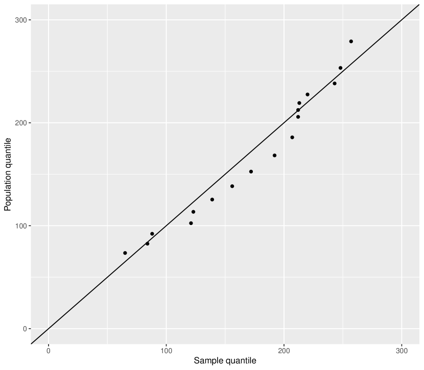
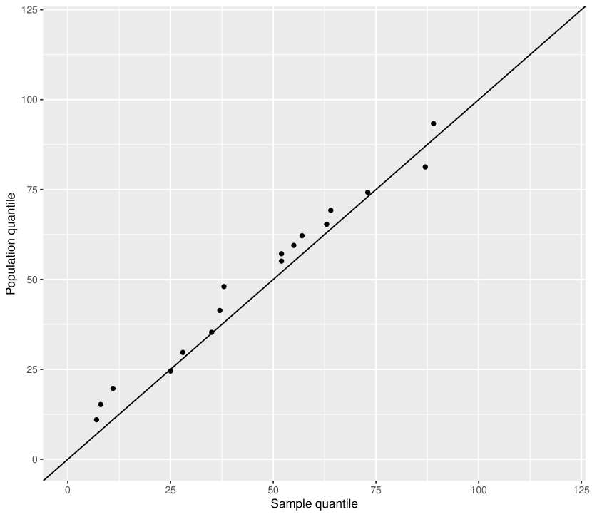
Sutar and Naik-Nimbalkar [34] observed that the load-sharing phenomenon existed for the systems considered in this dataset. Asha et al. [2] assumed Weibull lifetimes for the components. From the Weibull Q-Q plots for the lifetimes of motor A and B reported in Asha et al. [2], it was observed that although the Weibull model assumption for the lifetimes of motor B was reasonable, the lifetimes of motor A did not follow a Weibull distribution. This motivated us to consider the PLA-based modelling approach for the lifetimes of the load-sharing systems in this case.

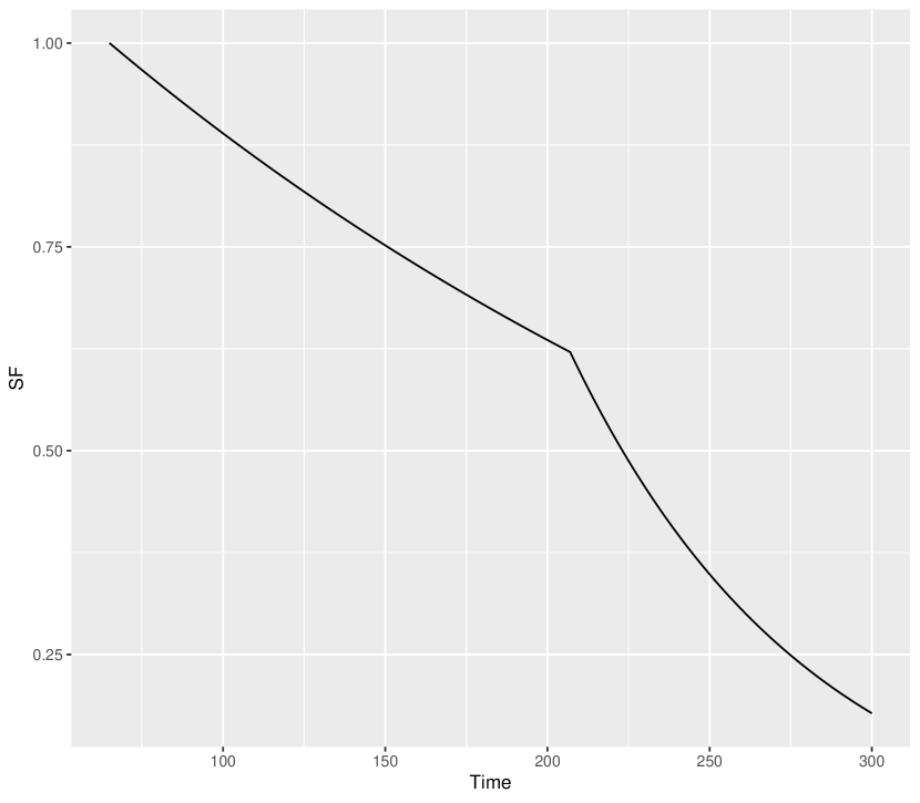
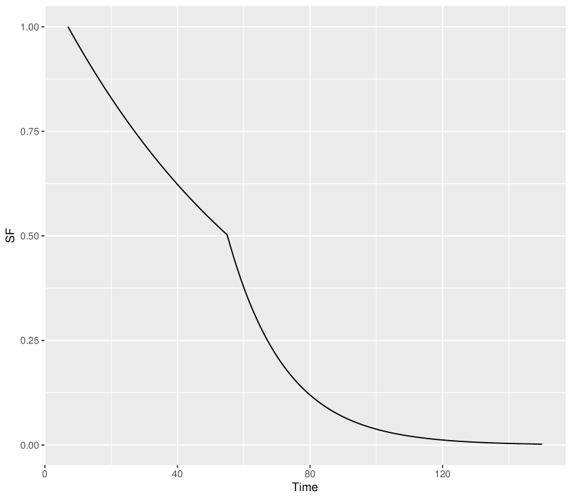
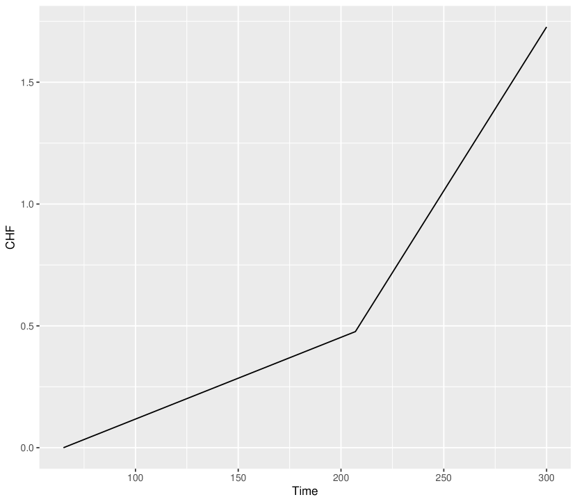
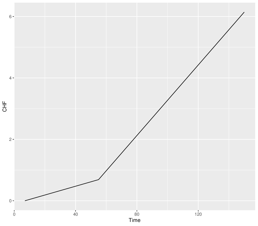
The dataset is reproduced in Table 1 for ready reference of the readers. The average and standard deviation of first component failure times are 178.61 and 62.75, respectively, while those of the lifetime between first and second component failures are 49.72 and 29.45, respectively. We consider three cut points for the PLA-based model (i.e., $N=2$ ). The estimates of the model parameters are reported in Table 2. The Q-Q plots for $Y^{(0)}$ and $Y^{(1)}$ are given in Figures 1(a) and 1(b), respectively. The plots of the estimated SF and CHF are given in Figures 2 and 3, respectively. These figures indicate that the PLA-based model fits the data quite adequately.

A Kolmogorov-Smirnov type test has been performed to test the following hypotheses:

\begin{array}[]{c}H_{0}:\text{ True model is specified by Eqs.\leavevmode\nobreak\ \eqref{eq:model1} and \eqref{eq:model2}}\\ \text{against}\\ H_{1}:\text{ True model is not specified by Eqs.\leavevmode\nobreak\ \eqref{eq:model1} and \eqref{eq:model2}}\end{array}

based on the test statistics

\displaystyle T_{n}=\max_{1\leq i\leq n}\left|\widehat{G}^{(0)}\left(Y^{(0)}_{i:n}\right)-\frac{i}{n}\right|+\max_{1\leq i\leq n}\left|\widehat{G}^{(1)}\left(Y^{(1)}_{i:n}\right)-\frac{i}{n}\right|,

where $\widehat{G}^{(j)}(\cdot)$ is the estimated cumulative distribution function corresponding to PLA-based model, and $Y^{(j)}_{i:n}$ is the $i$ -th order statistics corresponding to $Y^{(j)}_{i}$ , $j=0,\,1$ , $i=1,\,2,\,\ldots,\,n$ . The observed value of the test statistics $T_{n}$ is found to be 0.414 based on this data. The Monte Carlo estimate of the corresponding $p$ -value is 0.71. Therefore, the null hypothesis cannot be rejected at significance level 0.05, and we conclude that it is quite reasonable to use the PLA-based model for this data.

It may also be noted here that for this data, the value of the Akaike’s information criterion (AIC) for the model considered by Asha et al. [2] is 480.50, and that for the best model considered by Franco et al. [11] is 409.65. In contrast, the AIC value for the PLA-based model turns out to be 369.34, implying that the PLA-based model is more suitable for the two-motor load-sharing systems data considered here.

For the PLA-based model, the estimated value of $\gamma_{1}$ is 4.2712, which empirically implies that the load-sharing model is quite appropriate in this case. The same comment can also be made from the plots, by noting that the plot of the SF of the distribution of time between first and second failure component times diminishes to zero more quickly compared to that of first component failure times in Figure 2.

The reliability characteristics of the two-motor load-sharing systems are also estimated by using the expressions and techniques described in Section 4. The MTTF is calculated to be 221.36 days. Monte Carlo estimates of the MRT and RMT are calculated at different sample percentile points of the system failure times and are presented in Table 3.

6 Simulation Study

The accuracy of the proposed PLA-based model in fitting data from load-sharing systems is of utmost importance as the subsequent estimation of reliability characteristics depends on the PLA-based model. In this section, we present results of a Monte Carlo simulation study that examines the performance of the proposed PLA-based model in two directions. First, based on samples generated from a parent process with piecewise linear CHF, we assess the performance of the proposed estimation method that is presented in Section 3. Then, the efficacy of the PLA-based model in fitting data generated from a parent process represented by some parametric models is also assessed. The simulations are carried out by using R software. For the simulations, we consider two-component load-sharing systems.

6.1 Assessing performance of the estimation method

To assess the performance of the estimation methods, we consider an underlying cumulative hazard that is made up of two linear pieces. To this effect, we generate samples from the model specified by Eqs.(2.2) and (2.3) with $J=2$ and $N=2$ . The true parameter values are taken to be $b_{1}=0.01,\,0.05$ ; $b_{2}=0.1,\,0.5$ ; $\gamma_{1}=5$ ; $\tau_{1}^{(0)}=\frac{\ln 2}{2b_{1}}$ ; $\tau_{1}^{(1)}=\frac{\ln 2}{\gamma_{1}b_{1}}$ . The estimation is performed based on samples of size $n=100$ and 200. The average estimates (AE), mean square errors (MSE), variance (VAR) of the MLEs based on 5000 Monte Carlo replications are reported in Tables 4, 5, and 6. The coverage percentage (CP) and average lengths (AL) of 95% confidence intervals are also reported in the same tables.

From the Tables 4, 5 and 6, we observe that the average estimates of $\gamma_{1},\leavevmode\nobreak\ b_{1}$ and $b_{2}$ are very close to the true values, and the MSEs as well as VARs are quite small as desired. It is also noticed that the performance of all the constructed confidence intervals is satisfactory. These results demonstrate that the proposed inferential techniques can accurately estimate the parameters of the PLA-based model.

Table 4: Performance measures for estimates of

\gamma_{1}

$n$	$b_{1}$	$b_{2}$	AE	MSE	VAR	Asymptotic		Percentile bootstrap		Bootstrap
$n$	$b_{1}$	$b_{2}$	AE	MSE	VAR	CP	AL	CP	AL	CP	AL
	0.01	0.1	5.0231	0.3388811	0.3384155	94.38	2.2566	99.94	2.2012	83.58	2.2156
	0.01	0.5	5.0178	0.2880872	0.2878297	95.84	2.2509	99.94	2.1278	86.68	2.1993
100	0.05	0.1	5.0209	0.3556721	0.3553026	93.98	2.2711	98.52	2.3093	88.60	2.3226
	0.05	0.5	5.0231	0.3388811	0.3384155	94.38	2.2566	99.94	2.2012	83.58	2.2156
	0.01	0.1	5.0144	0.1472563	0.1470773	96.20	1.5963	99.90	1.5000	85.06	1.5093
	0.01	0.5	5.0127	0.1373738	0.1372388	96.64	1.5949	99.86	1.4395	84.42	1.4476
200	0.05	0.1	5.0145	0.1698002	0.1696241	94.84	1.6037	98.56	1.6165	89.56	1.6246
	0.05	0.5	5.0144	0.1472563	0.1470773	96.20	1.5963	99.90	1.5000	85.06	1.5093

Table 5: Performance measures for estimates of

b_{1}

$n$	$b_{1}$	$b_{2}$	AE	MSE	VAR	Asymptotic		Percentile bootstrap		Bootstrap
$n$	$b_{1}$	$b_{2}$	AE	MSE	VAR	CP	AL	CP	AL	CP	AL
	0.01	0.1	0.0108	0.0000022	0.0000016	87.24	0.0041	81.66	0.0052	92.88	0.0052
	0.01	0.5	0.0110	0.0000025	0.0000016	84.56	0.0042	68.70	0.0053	93.96	0.0054
100	0.05	0.1	0.0513	0.0000389	0.0000371	90.10	0.0201	95.96	0.0245	93.70	0.0246
	0.05	0.5	0.0528	0.0000457	0.0000376	89.18	0.0203	89.88	0.0252	92.70	0.0253
	0.01	0.1	0.0105	0.0000010	0.0000008	86.42	0.0029	81.74	0.0035	93.48	0.0036
	0.01	0.5	0.0106	0.0000011	0.0000008	84.74	0.0029	74.08	0.0036	94.56	0.0036
200	0.05	0.1	0.0508	0.0000186	0.0000180	90.06	0.0140	95.14	0.0169	93.08	0.0169
	0.05	0.5	0.0525	0.0000255	0.0000193	86.42	0.0143	81.74	0.0177	93.48	0.0178

Table 6: Performance measures for estimates of

b_{2}

$n$	$b_{1}$	$b_{2}$	AE	MSE	VAR	Asymptotic		Percentile bootstrap		Bootstrap
$n$	$b_{1}$	$b_{2}$	AE	MSE	VAR	CP	AL	CP	AL	CP	AL
	0.01	0.1	0.1006	0.0001691	0.0001688	92.70	0.0464	96.60	0.0534	94.00	0.0530
	0.01	0.5	0.5067	0.0038339	0.0037895	94.52	0.2344	97.12	0.2675	95.12	0.2676
100	0.05	0.1	0.1030	0.0001794	0.0001705	93.76	0.0472	95.46	0.0529	94.70	0.0532
	0.05	0.5	0.5028	0.0042337	0.0042268	92.68	0.2315	96.34	0.2650	94.00	0.2633
	0.01	0.1	0.1002	0.0000725	0.0000725	94.22	0.0325	96.72	0.0343	93.76	0.0345
	0.01	0.5	0.5030	0.0017348	0.0017261	95.06	0.1632	96.52	0.1665	93.60	0.1674
200	0.05	0.1	0.1011	0.0000780	0.0000768	93.84	0.0326	96.10	0.0351	94.08	0.0352
	0.05	0.5	0.5010	0.0018134	0.0018128	94.22	0.1623	96.72	0.1717	93.76	0.1725

Table 7: AIE based on SF and CHF for Weibull distribution with

k=3

\beta=1

$n$	$\alpha$	$AIE^{(0)}_{SF}$	$AIE^{(1)}_{SF}$	$AIE^{(0)}_{CHF}$	$AIE^{(1)}_{CHF}$
50	1.0	0.0379	0.0291	0.1503	0.2981
50	1.5	0.0436	0.0434	0.1329	0.2633
100	1.0	0.0266	0.0183	0.1282	0.2541
100	1.5	0.0326	0.0301	0.1231	0.2440

Table 8: AIE of the survival and cumulative hazard function of quadratic distribution for

\kappa_{1}=0.5,\leavevmode\nobreak\ \tilde{\kappa}_{1}=2\kappa_{1}=1,\leavevmode\nobreak\ \tilde{\kappa}_{2}>2\kappa_{2}

$n$	$\kappa_{2}$	$\tilde{\kappa}_{2}$	$AIE_{SF}^{(0)}$	$AIE_{SF}^{(1)}$	$AIE_{CHF}^{(0)}$	$AIE_{CHF}^{(1)}$
50	0.50	1.50	0.0380	0.0368	0.1262	0.2536
	0.50	2.00	0.0380	0.0389	0.1261	0.2555
	0.70	1.50	0.0389	0.0363	0.1261	0.2524
	0.70	2.00	0.0388	0.0383	0.1258	0.2539
100	0.50	1.50	0.0289	0.0262	0.1185	0.2506
	0.50	2.00	0.0289	0.0281	0.1178	0.2575
	0.70	1.50	0.0301	0.0257	0.1217	0.2465
	0.70	2.00	0.0299	0.0274	0.1206	0.2528

Table 9: AIE of the survival and cumulative hazard function of quadratic distribution for

\tilde{\kappa}_{1}>2\kappa_{1},\leavevmode\nobreak\ \kappa_{2}=0.5,\leavevmode\nobreak\ \tilde{\kappa}_{2}=2\kappa_{2}=1

$n$	$\kappa_{1}$	$\tilde{\kappa}_{1}$	$AIE_{SF}^{(0)}$	$AIE_{SF}^{(1)}$	$AIE_{CHF}^{(0)}$	$AIE_{CHF}^{(1)}$
50	0.50	1.50	0.0388	0.0313	0.1283	0.2570
	0.50	2.00	0.0397	0.0307	0.1309	0.2672
	0.70	1.50	0.0372	0.0314	0.1284	0.2567
	0.70	2.00	0.0377	0.0304	0.1301	0.2644
100	0.50	1.50	0.0306	0.0210	0.1265	0.2290
	0.50	2.00	0.0319	0.0206	0.1325	0.2285
	0.70	1.50	0.0278	0.0210	0.1184	0.2331
	0.70	2.00	0.0285	0.0198	0.1227	0.2271

6.2 Assessing efficacy of the PLA-based model in fitting data from other models

Now, we examine the robustness of the PLA-based model in the following manner. We generate load-sharing data from parametric models, and then fit the PLA-based model to the data. The model fit is then assessed with respect to an integrated measure that is suitably defined to reflect the quality of approximation provided by the PLA-based model. The measure, which we call the Absolute Integrated Error (AIE), is as follows. For $j=0,\,1$ , let $S^{(j)}_{TGP}(\cdot)$ and $H^{(j)}_{TGP}(\cdot)$ denote the SF and CHF of the lifetimes between $j$ -th and $(j+1)$ -st failures. Also, assume that the estimated SF and CHF based on PLA-based model are denoted by $\widehat{S}^{(j)}_{PLA}(\cdot)$ and $\widehat{H}^{(j)}_{PLA}(\cdot)$ , respectively. Then the AIE, based on the SF and CHF, respectively, are defined as

	$\displaystyle AIE_{SF}^{(j)}$	$\displaystyle=\frac{1}{R}\sum_{k=1}^{R}\frac{1}{y^{(j)}_{\max}-y^{(j)}_{\min}}\int_{y^{(j)}_{\min}}^{y^{(j)}_{\max}}\left\|S_{TGP}^{(j)}(t)-\widehat{S}_{PCA}^{(j)}(t)\right\|dt,$
	$\displaystyle AIE_{CHF}^{(j)}$	$\displaystyle=\frac{1}{R}\sum_{k=1}^{R}\frac{1}{y^{(j)}_{\max}-y^{(j)}_{\min}}\int_{y^{(j)}_{\min}}^{y^{(j)}_{\max}}\left\|H_{TGP}^{(j)}(t)-\widehat{H}_{PCA}^{(j)}(t)\right\|dt,$

where $y^{(j)}_{\min}=\min\left\{y^{(j)}_{1},\,y^{(j)}_{2},\,\ldots,\,y^{(j)}_{n}\right\}$ , $y^{(j)}_{\max}=\max\left\{y^{(j)}_{1},\,y^{(j)}_{2},\,\ldots,\,y^{(j)}_{n}\right\}$ , $j=0,\,1$ .

For generating load-sharing data from parametric models, two scenarios are considered:
(a) Case - 1: It is assumed that the lifetimes of each components of a two-component load-sharing system are independent and identically distributed as Weibull distribution with shape parameter $\alpha$ and scale parameter $\beta$ when both the components are working. After the first failure, the lifetime of the surviving component is assumed to follow a Weibull distribution with same shape parameter $\alpha$ , but a different scale parameter $k\beta$ , where $k>2$ is to ensure the increase of load on the surviving component. For $\beta=1$ , $k=3$ , we take $\alpha=1$ and 1.5.

(b) Case - 2: In the second scenario, the component lifetimes are assumed to be independent and identically distributed according to a distribution with quadratic CHF $\kappa_{1}t+\kappa_{2}t^{2}$ when both components are working. After the first failure, the lifetime of the surviving component is assumed to follow a quadratic CHF with different parameters $\tilde{\kappa}_{1}$ and $\tilde{\kappa}_{2}$ . We take several values of the parameters $\kappa_{1},\,\kappa_{2},\,\tilde{\kappa}_{1},$ and $\tilde{\kappa}_{2}$ ensuring the fact that the CHF increases after one component fails in the system.

The numerical results are reported in Tables 7, 8, and 9. For all cases, it is observed that the values of AIE based on SF and CHF are reasonably small, indicating that the PLA-based model provides quite a satisfactory approximation to the data generated from different parent populations.

7 Concluding Remarks

In this article, a PLA-based model for the CHF is proposed for data from load-sharing systems and then important reliability characteristics such as quantile function, RMT, MTTF, and MRT of load-sharing systems are estimated under the proposed model. The principal advantages of the model are that it is data-driven, and does not use strong parametric assumptions for the underlying lifetime variable. Likelihood inference for the proposed model is discussed in detail. It is observed that for two-component load-sharing systems, it is possible to obtain explicit expressions for the MLEs of parameters of the PLA-based model. Construction of confidence intervals using the Fisher information matrix and bootstrap approaches are also discussed. Derivations of the important reliability characteristics are provided in this setting.

A Monte Carlo simulation study is performed to examine (a) the performance of the methods of inference, and (b) the efficacy of the PLA-based model to fit load-sharing data in general. It is shown that the PLA-based model performs quite satisfactorily in both cases. Analysis of data pertaining to components lifetimes of a two-motor load-sharing system is provided as an illustration. It is illustrated that the PLA-based model is superior to the models that have been considered for this data in the literature of load-sharing systems. In summary, in this paper, an efficient PLA-based modelling framework using minimal assumptions for load-sharing systems is discussed, and estimates of important reliability characteristics for load-sharing systems in this setting are developed.

Funding information

•

The research of Ayon Ganguly is supported by the Mathematical Research Impact Centric Support (File no. MTR/2017/000700) from the Science and Engineering Research Board, Department of Science and Technology, Government of India.
•

The research of Debanjan Mitra is supported by the Mathematical Research Impact Centric Support (File no. MTR/2021/000533) from the Science and Engineering Research Board, Department of Science and Technology, Government of India.

References

[1] S.V. Amari and R. Bergman. Reliability analysis of $k$ -out-of- $n$ load-sharing systems. In Annual Reliability and Maintainability Symposium, pages 440–445, 2008.
[2] G Asha, AV Raja, and N. Ravishanker. Reliability modelling incorporating load share and frailty. Applied Stochastic Models in Business and Industry, 34:206–223, 2018.
[3] N. Balakrishnan, M. Koutras, F. Milienos, and S. Pal. Piecewise linear approximations for cure rate models. Methodology and Computing in Applied Probability, 18(4):937–966, 2016.
[4] C.D. Bernard. Time dependence of mechanical breakdown in bundles of fibers. I. constant total load. Journal of Applied Physics, 28(9):1058–1064, 1957.
[5] C.D. Bernard. Statistics and time dependence of mechanical breakdown in fibers. Journal of Applied Physics, 29(6):968–983, 1958.
[6] Z. W. Birnbaum and S. C. Saunders. A statistical model for life-length of materials. Journal of the American Statistical Association, 53(281):151–160, 1958.
[7] B. Brown, B. Liu, S. McIntyre, and M. Revie. Reliability analysis of load-sharing systems with spatial dependence and proximity effects. Reliability Engineering and System Safety, 2022.
[8] H. Che, S. Zeng, K. Li, and J. Guo. Reliability analysis of load-sharing man-machine systems subject to machine degradation, human errors, and random shocks. Reliability Engineering and System Safety, 2022.
[9] H.E. Daniels. The statistical theory of the strength of bundles of threads I. Proceedings of the Royal Society of London, 83:405–435, 1945.
[10] JV Deshpande, I. Dewan, and UV Naik-Nimbalkar. A family of distributions to model load sharing systems. Journal of Statistical Planning and Inference, 140:1441–1451, 2010.
[11] M Franco, JM Vivo, and D Kundu. A generalized Freund bivariate model for a two-component load sharing system. Reliability Engineering and System Safety, 2020.
[12] JE Freund. A bivariate extension of the exponential distribution. Journal of American Statistical Association, 56:971–976, 1961.
[13] D. G. Harlow and S. L. Phoenix. The chain-of-bundles probability model for the strength of fibrous materials I: analysis and conjectures. Journal of composite materials, 12(2):195–214, 1978.
[14] D. G. Harlow and S. L. Phoenix. Probability distributions for the strength of fibrous materials under local load sharing I: two-level failure and edge effects. Advances in Applied Probability, pages 68–94, 1982.
[15] M. Hollander and E. A. Pena. Dynamic reliability models with conditional proportional hazards. Lifetime Data Analysis, 1(4):377–401, 1995.
[16] H. Kim and P.H. Kvam. Reliability estimation based on system data with an unknown load share rule. Lifetime Data Analysis, 10:83–94, 2004.
[17] Y. Kong and Z. S. Ye. A cumulative-exposure-based algorithm for failure data from a load-sharing system. IEEE Transactions on Reliability, 65(2):1001–1012, 2016.
[18] H. P. Kvam and J. C. Lu. Load-sharing models. Math and Computer Science Faculty Publications, 2008.
[19] S. Lee, S. Durham, and J. Lynch. On the calculation of the reliability of general load sharing system. Journal of Applied Probability, 32:777–792, 1995.
[20] H.H. Lin, K.H. Chen, and R.T. Wang. A multivariant exponential shared-load model. IEEE Transactions on Reliability, 42(1):165–171, 1993.
[21] C. Luo, L. Chen, and A. Xu. Modelling and estimation of system reliability under dynamic operating environments and lifetime ordering constraints. Reliability Engineering and System Safety, 2022.
[22] J D Lynch. On the joint distribution of component failures for monotone load-sharing systems. Journal of Statistical Planning and Inference, 78:13–21, 1999.
[23] A. Mettas and P. Vassiliou. Application of quantitative accelerated life models on load sharing redundancy. In Annual Symposium Reliability and Maintainability, 2004-RAMS, pages 293–296. IEEE, 2004.
[24] R. Mohammad, A. Kalam, and S.V. Amari. Reliability evaluation of phased-mission systems with load-sharing components. In Proceedings Annual Reliability and Maintainability Symposium, pages 1–6. IEEE, 2012.
[25] C. H. Muller and R. Meyer. Inference of intensity-based models for load-sharing systems with damage accumulation. IEEE Transactions on Reliability, 71:539–554, 2012.
[26] E. Nezakati and M. Ramzakh. Reliability analysis of a load sharing $k$ -out-of- $n$ :f degradation system with dependent competing failures. Reliability Engineering and System Safety, 2020.
[27] C. Park. Parameter estimation for the reliability of load-sharing systems. IIE Transactions, 42:753–765, 2010.
[28] C. Park. Parameter estimation from load-sharing system data using the expectation-maximization algorithm. IIE Transactions, 45:147–163, 2013.
[29] B. W. Rosen. Tensile failure of fibrous composites. AIAA journal, 2(11):1985–1991, 1964.
[30] S.M. Ross. A model in which component failure rates depend on the working set. Naval research logistics quarterly, 31(2):297–300, 1984.
[31] Z. Schechner. A load-sharing model: The linear breakdown rule. Naval research logistics quarterly, 31(1):137–144, 1984.
[32] J. Shao and L.R. Lamberson. Modeling a shared-load $k$ -out-of- $n$ : G system. IEEE Transactions on Reliability, 40(2):205–209, 1991.
[33] A.V. Suprasad, M.B. Krishna, and P. Hoang. Tampered failure rate load-sharing systems: Status and perspectives. In Handbook of performability engineering, pages 291–308. Springer, 2008.
[34] S S Sutar and U V Naik-Nimbalkar. Accelerated failure time models for load sharing systems. IEEE Transactions on Reliability, 63:706–714, 2014.
[35] J. Zhang, Y. Zhao, and X. Ma. Reliability modeling methods for load-sharing $k$ -out-of- $n$ system subject to discrete external load. Reliability Engineering and System Safety, 2020.
[36] X. Zhao, B. Liu, and Y. Liu. Reliability modeling and analysis of load-sharing systems with continuously degrading components. IEEE Transactions on Reliability, 67:1096–1110, 2018.

Appendix A: Calculation of Fisher information matrix for two-component load sharing systems

For calculating $\mathbb{I}(\boldsymbol{\theta})$ , the required expectations are $E\left(N_{1}^{(0)}\right),E\left(N_{2}^{(0)}\right),E\left(N_{1}^{(1)}\right),E\left(N_{2}^{(1)}\right),\\ E\left(\displaystyle\sum_{i\in I_{1}^{(1)}}Y_{i}^{(1)}\right)$ and $E\left(\displaystyle\sum_{i\in I_{2}^{(1)}}Y_{i}^{(1)}\right)$ .
Note that

N_{k}^{(0)}\sim Bin(n,p_{k}^{(0)}),\quad N_{k}^{(1)}\sim Bin(n,p_{k}^{(1)}),

with

p_{k}^{(0)}=P\bigg{(}Y_{i}^{(0)}\in[\tau_{k-1}^{(0)},\tau_{k}^{(0)})\bigg{)},\quad p_{k}^{(1)}=P\bigg{(}Y_{i}^{(1)}\in[\tau_{k-1}^{(1)},\tau_{k}^{(1)})\bigg{)},\quad k=1,2.

In case of a two-component load-sharing system, PDF of $Y_{i}^{(j)}$ , $j=1,2$ , is given by

\displaystyle g_{Y_{i}^{(j)}}(y)=(2-j)\lambda^{(j)}(y)e^{-(2-j)\int_{0}^{y}\lambda^{(j)}(u)du}.

Hence,

\displaystyle p_{1}^{(0)}=\int_{0}^{\tau_{1}^{(0)}}g_{Y_{i}^{(0)}}(y)dy=1-e^{-2b_{1}\tau_{1}^{(0)}},\quad p_{1}^{(1)}=\int_{0}^{\tau_{1}^{(1)}}g_{Y_{i}^{(1)}}(y)dy=1-e^{-\gamma_{1}b_{1}\tau_{1}^{(1)}}.

Then, $p_{2}^{(0)}=1-p_{1}^{(0)}=e^{-2b_{1}\tau_{1}^{(0)}}$ and $p_{2}^{(1)}=1-p_{1}^{(1)}=e^{-\gamma_{1}b_{1}\tau_{1}^{(1)}}$ . Therefore,

E(N_{1}^{(0)})=1-e^{-2b_{1}\tau_{1}^{(0)}},\quad E(N_{2}^{(0)})=e^{-2b_{1}\tau_{1}^{(0)}},\quad E(N_{1}^{(1)})=1-e^{-\gamma_{1}b_{1}\tau_{1}^{(1)}},\quad E(N_{2}^{(1)})=e^{-\gamma_{1}b_{1}\tau_{1}^{(1)}}.

Now,

E\left(\sum_{i\in I_{1}^{(1)}}Y_{i}^{(1)}\right)=E\left(E\left(\sum_{i\in I_{1}^{(1)}}Y_{i}^{(1)}|N_{1}^{(1)}=n_{1}^{(1)}\right)\right).

For $i\in I_{1}^{(1)}$ , $Y_{i}^{(1)}$ follows a right truncated exponential distribution with PDF $\frac{\gamma_{1}b_{1}e^{-\gamma_{1}b_{1}y}}{1-e^{-\gamma_{1}b_{1}\tau_{1}^{(1)}}}$ for $0<y<\tau_{1}^{(1)}$ . Hence, for $i\in I_{1}^{(1)}$ ,

E\left(Y_{i}^{(1)}\right)=\int_{0}^{\tau_{1}^{(1)}}y\frac{\gamma_{1}b_{1}e^{-\gamma_{1}b_{1}y}}{1-e^{-\gamma_{1}b_{1}\tau_{1}^{(1)}}}dy=\frac{1}{\gamma_{1}b_{1}}\left[\frac{1-(1+\gamma_{1}b_{1}\tau_{1}^{(1)})e^{-\gamma_{1}b_{1}\tau_{1}^{(1)}}}{1-e^{-\gamma_{1}b_{1}\tau_{1}^{(1)}}}\right].

Therefore,

	$\displaystyle E\left(\sum_{i\in I_{1}^{(1)}}Y_{i}^{(1)}\right)$	$\displaystyle=\frac{1}{\gamma_{1}b_{1}}\left[\frac{1-(1+\gamma_{1}b_{1}\tau_{1}^{(1)})e^{-\gamma_{1}b_{1}\tau_{1}^{(1)}}}{1-e^{-\gamma_{1}b_{1}\tau_{1}^{(1)}}}\right]E(N_{1}^{(1)})$
		$\displaystyle=\frac{1}{\gamma_{1}b_{1}}\left[\frac{1-(1+\gamma_{1}b_{1}\tau_{1}^{(1)})e^{-\gamma_{1}b_{1}\tau_{1}^{(1)}}}{1-e^{-\gamma_{1}b_{1}\tau_{1}^{(1)}}}\right]\left(1-e^{-\gamma_{1}b_{1}\tau_{1}^{(1)}}\right)$
		$\displaystyle=\frac{1}{\gamma_{1}b_{1}}\left[{1-(1+\gamma_{1}b_{1}\tau_{1}^{(1)})e^{-\gamma_{1}b_{1}\tau_{1}^{(1)}}}\right].$

Similarly,

E\left(\sum_{i\in I_{2}^{(1)}}Y_{i}^{(1)}\right)=E\left(E\left(\sum_{i\in I_{2}^{(1)}}Y_{i}^{(1)}|N_{2}^{(1)}=n_{2}^{(1)}\right)\right).

For $i\in I_{2}^{(1)}$ , $Y_{i}^{(1)}$ follows a left truncated exponential distribution with PDF $\frac{\gamma_{1}b_{2}e^{-\gamma_{1}b_{2}y}}{e^{-\gamma_{1}b_{2}\tau_{1}^{(1)}}}$ for $y>\tau_{1}^{(1)}$ . Hence,

E\left(Y_{i}^{(1)}\right)=\int_{\tau_{1}^{(1)}}^{\infty}y\frac{\gamma_{1}b_{2}e^{-\gamma_{1}b_{2}y}}{e^{-\gamma_{1}b_{2}\tau_{1}^{(1)}}}dy=\frac{1}{\gamma_{1}b_{2}}+\tau_{1}^{(1)}.

Therefore,

E\left(\sum_{i\in I_{2}^{(1)}}Y_{i}^{(1)}\right)=\left(\frac{1}{\gamma_{1}b_{2}}+\tau_{1}^{(1)}\right)E(N_{2}^{(1)})=\left(\frac{1}{\gamma_{1}b_{2}}+\tau_{1}^{\prime}\right)e^{-\gamma_{1}b_{1}\tau_{1}^{(1)}}.

Appendix B: Calculations of some important reliability characteristics

Derivation of the quantile function:

Denote $p=G^{(j)}(y)$ for $y\in\left[\tau_{k-1}^{(j)},\tau_{k}^{(j)}\right)$ ; then, $y=\eta(p)$ for $p\in\left[G^{(j)}(\tau_{k-1}^{(j)}),G^{(j)}(\tau_{k}^{(j)})\right)$ , $k=1,2,\ldots,N.$ Now,

	$\displaystyle p$	$\displaystyle=1-e^{-(J-j)\gamma_{j}\left[\sum_{\ell=1}^{k-1}b_{\ell}\left(\tau_{\ell}^{(j)}-\tau_{\ell-1}^{(j)}\right)+b_{k}\left(y-\tau_{k-1}^{(j)}\right)\right]}$
	$\displaystyle\implies$	$\displaystyle b_{k}\left(y-\tau_{k-1}^{(j)}\right)=-\frac{\log(1-p)}{(J-j)\gamma_{j}}-\sum_{\ell=1}^{k-1}b_{\ell}\left(\tau_{\ell}^{(j)}-\tau_{\ell-1}^{(j)}\right)$
	$\displaystyle\implies$	$\displaystyle y=\tau_{k-1}^{(j)}-\frac{\log(1-p)}{(J-j)\gamma_{j}b_{k}}-\frac{1}{b_{k}}\sum_{\ell=1}^{k-1}b_{\ell}\left(\tau_{\ell}^{(j)}-\tau_{\ell-1}^{(j)}\right),\text{ if }p\in\left[G^{(j)}(\tau_{k-1}^{(j)}),G^{(j)}(\tau_{k}^{(j)})\right),$
		$\displaystyle\hskip 256.0748ptk=1,2,\ldots,N.$

If $y\in\left[\tau_{N}^{(j)},\infty\right)$ , then $y=\eta(p)$ for $p\in\left[G^{(j)}(\tau_{N}^{(j)}),1\right)$ .
Therefore,

	$\displaystyle p$	$\displaystyle=1-e^{-(J-j)\gamma_{j}\left[\sum_{\ell=1}^{N-1}b_{\ell}\left(\tau_{\ell}^{(j)}-\tau_{\ell-1}^{(j)}\right)+b_{N}\left(y-\tau_{N-1}^{(j)}\right)\right]}$
	$\displaystyle\implies$	$\displaystyle y=\tau_{N-1}^{(j)}-\frac{\log(1-p)}{(J-j)\gamma_{j}b_{N}}-\frac{1}{b_{N}}\sum_{\ell=1}^{N-1}b_{\ell}\left(\tau_{\ell}^{(j)}-\tau_{\ell-1}^{(j)}\right),\text{ if }p\in\left[G^{(j)}(\tau_{N}^{(j)}),1\right).$

Derivation of MTTF:

MTTF of the system lifetime $T$ is given by $E(T)=E\left(\displaystyle\sum_{j=0}^{J-1}Y^{(j)}\right)=\displaystyle\sum_{j=0}^{J-1}E(Y^{(j)})$ , where

E(Y^{(j)})=\int_{0}^{\infty}P(Y^{(j)}>y)dy=\int_{0}^{\tau_{N-1}^{(j)}}e^{-(J-j)\Lambda^{(j)}(y)}dy+\int_{\tau_{N-1}^{(j)}}^{\infty}e^{-(J-j)\Lambda^{(j)}(y)}dy=I_{1}+I_{2}\;(\textrm{say}).

Here,

	$\displaystyle I_{1}$	$\displaystyle=\int_{0}^{\tau_{N-1}^{(j)}}e^{-(J-j)\gamma_{j}\sum_{k=1}^{N}\left[\sum_{\ell=1}^{k-1}b_{\ell}\left(\tau_{\ell}^{(j)}-\tau_{\ell-1}^{(j)}\right)+b_{k}\left(y-\tau_{k-1}^{(j)}\right)\right]\boldsymbol{1}_{[\tau^{(0)}_{k-1},\,\tau^{(0)}_{k})}\left(y\right)}dy$
		$\displaystyle=\sum_{s=1}^{N-1}\int_{\tau_{s-1}^{(j)}}^{\tau_{s}^{(j)}}e^{-(J-j)\gamma_{j}\left[\sum_{\ell=1}^{s-1}b_{\ell}\left(\tau_{\ell}^{(j)}-\tau_{\ell-1}^{(j)}\right)+b_{s}\left(y-\tau_{s-1}^{(j)}\right)\right]}dy$
		$\displaystyle=\sum_{s=1}^{N-1}\left\{e^{-(J-j)\gamma_{j}\sum_{\ell=1}^{s-1}b_{\ell}\left(\tau_{\ell}^{(j)}-\tau_{\ell-1}^{(j)}\right)}\int_{\tau_{s-1}^{(j)}}^{\tau_{s}^{(j)}}e^{-(J-j)\gamma_{j}b_{s}\left(y-\tau_{s-1}^{(j)}\right)}dy\right\}$
		$\displaystyle=\sum_{s=1}^{N-1}\left\{e^{-(J-j)\gamma_{j}\sum_{\ell=1}^{s-1}b_{\ell}\left(\tau_{\ell}^{(j)}-\tau_{\ell-1}^{(j)}\right)}\left[\frac{1-e^{-(J-j)\gamma_{j}b_{s}\left(\tau_{s}^{(j)}-\tau_{s-1}^{(j)}\right)}}{(J-j)\gamma_{j}b_{s}}\right]\right\}$
		$\displaystyle=\sum_{s=1}^{N-1}\left\{\frac{e^{-(J-j)\gamma_{j}\sum_{\ell=1}^{s-1}b_{\ell}\left(\tau_{\ell}^{(j)}-\tau_{\ell-1}^{(j)}\right)}-e^{-(J-j)\gamma_{j}\sum_{\ell=1}^{s}b_{\ell}\left(\tau_{\ell}^{(j)}-\tau_{\ell-1}^{(j)}\right)}}{(J-j)\gamma_{j}b_{s}}\right\}$

and

	$\displaystyle I_{2}$	$\displaystyle=\int_{\tau_{N-1}^{(j)}}^{\infty}e^{-(J-j)\gamma_{j}\sum_{k=1}^{N}\left[\sum_{\ell=1}^{k-1}b_{\ell}\left(\tau_{\ell}^{(j)}-\tau_{\ell-1}^{(j)}\right)+b_{k}\left(y-\tau_{k-1}^{(j)}\right)\right]\boldsymbol{1}_{[\tau^{(0)}_{k-1},\,\tau^{(0)}_{k})}\left(y\right)}dy$
		$\displaystyle=\int_{\tau_{N-1}^{(j)}}^{\infty}e^{-(J-j)\gamma_{j}\left[\sum_{\ell=1}^{N-1}b_{\ell}\left(\tau_{\ell}^{(j)}-\tau_{\ell-1}^{(j)}\right)+b_{N}\left(y-\tau_{N-1}^{(j)}\right)\right]}dy$
		$\displaystyle=e^{-(J-j)\gamma_{j}\sum_{\ell=1}^{N-1}b_{\ell}\left(\tau_{\ell}^{(j)}-\tau_{\ell-1}^{(j)}\right)}\int_{\tau_{N-1}^{(j)}}^{\infty}e^{-(J-j)\gamma_{j}b_{N}\left(y-\tau_{N-1}^{(j)}\right)}dy$
		$\displaystyle=e^{-(J-j)\gamma_{j}\sum_{\ell=1}^{N-1}b_{\ell}\left(\tau_{\ell}^{(j)}-\tau_{\ell-1}^{(j)}\right)}\left[\frac{1}{(J-j)\gamma_{j}b_{N}}\right]$
		$\displaystyle=\frac{e^{-(J-j)\gamma_{j}\sum_{\ell=1}^{N-1}b_{\ell}\left(\tau_{\ell}^{(j)}-\tau_{\ell-1}^{(j)}\right)}}{(J-j)\gamma_{j}b_{N}}.$

Therefore,

\displaystyle E(Y^{(j)})=\sum_{s=1}^{N}\left\{\frac{e^{-(J-j)\gamma_{j}\sum_{\ell=1}^{s-1}b_{\ell}\left(\tau_{\ell}^{(j)}-\tau_{\ell-1}^{(j)}\right)}-e^{-(J-j)\gamma_{j}\sum_{\ell=1}^{s}b_{\ell}\left(\tau_{\ell}^{(j)}-\tau_{\ell-1}^{(j)}\right)}}{(J-j)\gamma_{j}b_{s}}\right\}.

From here, the results follows immediately.

Derivation of moment generating function of system lifetime:

Note that the system lifetime MGF of $T$ is $T=\displaystyle\sum_{j=0}^{J-1}Y^{(j)}$ , where $Y^{(j)}$ ’s are independent for $j=0,1,\ldots,(J-1)$ . Therefore, the MGF of $T$ is $\phi_{T}(t)=\displaystyle\prod_{j=0}^{J-1}\phi_{Y^{(j)}}(t)$ . Now,

		$\displaystyle\phi_{Y^{(j)}}(t)$	$\displaystyle=E(e^{tY^{(j)}})=\int_{0}^{\infty}e^{ty}g_{Y^{(j)}}(y)dy$
			$\displaystyle=\int_{0}^{\tau_{N-1}^{(j)}}e^{ty}(J-j)\lambda^{(j)}(y)e^{-(J-j)\Lambda^{(j)}(y)}dy+\int_{\tau_{N-1}^{(j)}}^{\infty}e^{ty}(J-j)\lambda^{(j)}(y)e^{-(J-j)\Lambda^{(j)}(y)}dy$
			$\displaystyle=I_{1}+I_{2}\text{ (say) },$

where $g_{Y^{(j)}}(y)=(J-j)\lambda^{(j)}(y)e^{-(J-j)\Lambda^{(j)}(y)}.$ For $t\in\mathbb{R}$ ,

	$\displaystyle I_{1}$	$\displaystyle=\int_{0}^{\tau_{N-1}^{(j)}}e^{ty}(J-j)\gamma_{j}\sum_{k=1}^{N}b_{k}\boldsymbol{1}_{[\tau^{(j)}_{k-1},\,\tau^{(j)}_{k})}\left(y\right)e^{-(J-j)\gamma_{j}\sum_{k=1}^{N}\left[\sum_{\ell=1}^{k-1}b_{\ell}\left(\tau_{\ell}^{(j)}-\tau_{\ell-1}^{(j)}\right)+b_{k}\left(y-\tau_{k-1}^{(j)}\right)\right]}dy$
		$\displaystyle=\sum_{s=1}^{N-1}(J-j)b_{s}\gamma_{j}\int_{\tau_{s-1}^{(j)}}^{\tau_{s}^{(j)}}e^{-\left\{(J-j)\gamma_{j}\left[\sum_{\ell=1}^{s-1}b_{\ell}\left(\tau_{\ell}^{(j)}-\tau_{\ell-1}^{(j)}\right)+b_{s}\left(y-\tau_{s-1}^{(j)}\right)\right]-ty\right\}}dy$
		$\displaystyle=\sum_{s=1}^{N-1}\left\{(J-j)b_{s}\gamma_{j}e^{-(J-j)\gamma_{j}\sum_{\ell=1}^{s-1}b_{\ell}\left(\tau_{\ell}^{(j)}-\tau_{\ell-1}^{(j)}\right)}\int_{\tau_{s-1}^{(j)}}^{\tau_{s}^{(j)}}e^{-\left\{(J-j)\gamma_{j}b_{s}\left(y-\tau_{s-1}^{(j)}\right)-ty\right\}}dy\right\}$
		$\displaystyle=\sum_{s=1}^{N-1}\left\{(J-j)b_{s}\gamma_{j}e^{-(J-j)\gamma_{j}\sum_{\ell=1}^{s-1}b_{\ell}\left(\tau_{\ell}^{(j)}-\tau_{\ell-1}^{(j)}\right)}\left[\frac{e^{t\tau_{s-1}^{(j)}}-e^{-\left\{(J-j)\gamma_{j}b_{s}\left(\tau_{s}^{(j)}-\tau_{s-1}^{(j)}\right)-t\tau_{s}^{(j)}\right\}}}{(J-j)\gamma_{j}b_{s}-t}\right]\right\}$
		$\displaystyle=\sum_{s=1}^{N-1}\frac{(J-j)b_{s}\gamma_{j}}{(J-j)b_{s}\gamma_{j}-t}\left\{e^{-\left\{(J-j)\gamma_{j}\sum_{\ell=1}^{s-1}b_{\ell}\left(\tau_{\ell}^{(j)}-\tau_{\ell-1}^{(j)}\right)-t\tau_{s-1}^{(j)}\right\}}\right.$
		$\displaystyle\hskip 170.71652pt\left.-e^{-\left\{(J-j)\gamma_{j}\sum_{\ell=1}^{s}b_{\ell}\left(\tau_{\ell}^{(j)}-\tau_{\ell-1}^{(j)}\right)-t\tau_{s}^{(j)}\right\}}\right\}.$

For $t<(J-j)\gamma_{j}b_{N}$ ,

	$\displaystyle I_{2}$	$\displaystyle=\int_{\tau_{N-1}^{(j)}}^{\infty}e^{ty}(J-j)\gamma_{j}\sum_{k=1}^{N}b_{k}\boldsymbol{1}_{[\tau^{(j)}_{k-1},\,\tau^{(j)}_{k})}\left(y\right)e^{-(J-j)\gamma_{j}\sum_{k=1}^{N}\left[\sum_{\ell=1}^{k-1}b_{\ell}\left(\tau_{\ell}^{(j)}-\tau_{\ell-1}^{(j)}\right)+b_{k}\left(y-\tau_{k-1}^{(j)}\right)\right]}dy$
		$\displaystyle=(J-j)b_{N}\gamma_{j}\int_{\tau_{N-1}^{(j)}}^{\infty}e^{ty-(J-j)\gamma_{j}\left[\sum_{\ell=1}^{N-1}b_{\ell}\left(\tau_{\ell}^{(j)}-\tau_{\ell-1}^{(j)}\right)+b_{N}\left(y-\tau_{N-1}^{(j)}\right)\right]}dy$
		$\displaystyle=(J-j)b_{N}\gamma_{j}e^{-(J-j)\gamma_{j}\sum_{\ell=1}^{N-1}b_{\ell}\left(\tau_{\ell}^{(j)}-\tau_{\ell-1}^{(j)}\right)}\int_{\tau_{N-1}^{(j)}}^{\infty}e^{-\left\{(J-j)\gamma_{j}b_{N}\left(y-\tau_{N-1}^{(j)}\right)-ty\right\}}dy$
		$\displaystyle=(J-j)b_{N}\gamma_{j}e^{-(J-j)\gamma_{j}\sum_{\ell=1}^{N-1}b_{\ell}\left(\tau_{\ell}^{(j)}-\tau_{\ell-1}^{(j)}\right)}\left[\frac{e^{t\tau_{N-1}^{(j)}}}{{(J-j)\gamma_{j}b_{N}-t}}\right]$
		$\displaystyle=(J-j)b_{N}\gamma_{j}\cdot\frac{e^{t\tau_{N-1}^{(j)}-(J-j)\gamma_{j}\sum_{\ell=1}^{N-1}b_{\ell}\left(\tau_{\ell}^{(j)}-\tau_{\ell-1}^{(j)}\right)}}{(J-j)b_{N}\gamma_{j}-t}.$

Therefore, for $t<(J-j)\gamma_{j}b_{N}$ ,

	$\displaystyle\phi_{Y^{(j)}}(t)=$	$\displaystyle\sum_{s=1}^{N}\frac{(J-j)b_{s}\gamma_{j}}{(J-j)b_{s}\gamma_{j}-t}\left\{e^{-\left\{(J-j)\gamma_{j}\sum_{\ell=1}^{s-1}b_{\ell}\left(\tau_{\ell}^{(j)}-\tau_{\ell-1}^{(j)}\right)-t\tau_{s-1}^{(j)}\right\}}\right.$
		$\displaystyle\hskip 142.26378pt\left.-e^{-\left\{(J-j)\gamma_{j}\sum_{\ell=1}^{s}b_{\ell}\left(\tau_{\ell}^{(j)}-\tau_{\ell-1}^{(j)}\right)-t\tau_{s}^{(j)}\right\}}\right\}.$

From here the result follows immediately.