Relativistic Wind Farm Effect: Possibly Turbulent Flow of a Charged, Massless Relativistic Fluid in Graphene

Graphene is a sheet of graphite, one carbon atom thick, with interesting physical and electrical properties. Its provides an excellent experimental platform to observe electric transport properties and test theories on conductivity at moderately high temperatures. The two-dimensional solid is made of carbon atoms arranged in a honeycomb lattice, showing a high conductivity through a simple band structure. Of focused interest is the charge neutral state where each carbon atom contains exactly one electron so that half of the energy levels are occupied. In this state the band gap disappears at points on the Fermi surface called Dirac points, and the dispersion relation is nearly linear surrounding the points and form a conical Fermi surface at low energies. Deviations from the linear dispersion begin to appear at a very high temperature, $\approx 10^{5}K$, validated experimentally in [1][2]. The electric charge is transported through the conical band structure by highly mobile, massless chiral quasi-particles [3] referred to as Dirac particles. The number density of the quasi-particles is determined using electrical properties such as the Hall resistance, which normally assumes an integer value in a two-dimensional solid, but in graphene is found in multiples of $1/2$, known as the fractional Quantum Hall Effect [4]. In the presence of a strong magnetic field the wave functions of the quasi-particles behave like simple quantum harmonic oscillators that take on discrete energy levels based on the strength of the magnetic field. This effect, called the Shubnikov-De Haas effect, is used to determine the effective mass of the charge carrying quasi-particles.

The dynamics of the quasi-particles constituting the electric current can be described collectively with hydrodynamics, but since the quasi-particles have no mass and are subject to Dirac’s equation their collective velocity distribution cannot be given by a Maxwell-Boltzmann distribution. Hence, despite having typical velocities much less than the speed of light, the flow of these particles is better described with relativistic hydrodynamics. Because of this the study of the electric current in graphene can also be applicable to some astrophysical systems such as gamma ray bursts, supernovae or the flow of particles around the event horizon of a black hole. These systems share the property of a relativistic hydrodynamic flow, but are of course, much less accessible to experiment. See [5] [6] for recent textbooks on relativistic hydrodynamics.

The transport of the charge carrying quasi-particles within graphene demonstrates a high conductivity that stays above a minimum value, even when carrier concentrations approach zero [3]. Additionally, the viscosity to entropy ratio is determined to be very small; smaller than that of superfluid helium [7]. A sample of graphene will contain impurities embedded within the honeycomb lattice structure or within the supporting substrate that will affect the current based on their number density, size, placement and electric properties. In a hydrodynamic flow, if the average fluid speed around these obstructions is large enough compared to the viscous damping effect, a turbulent flow is possible.

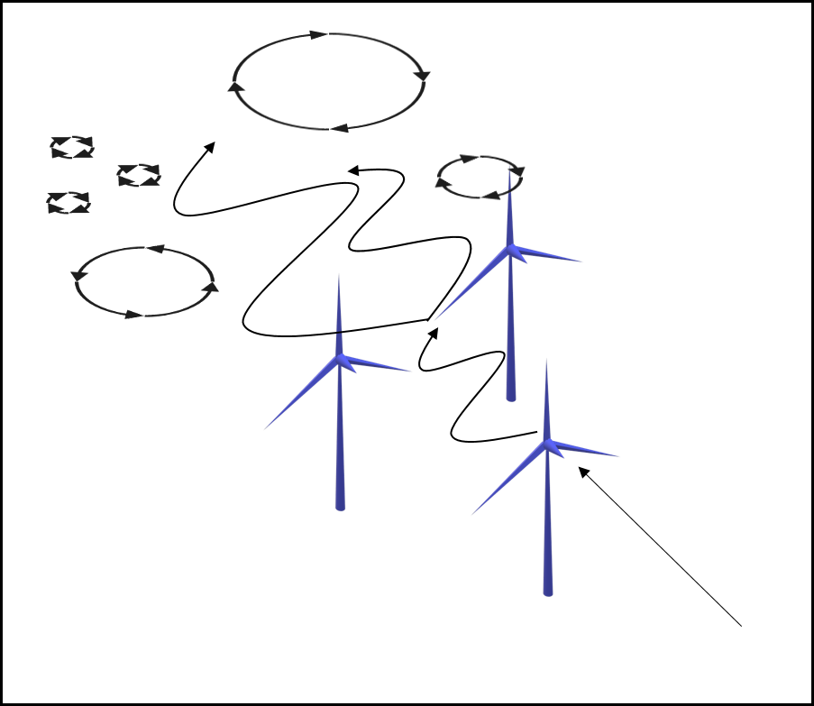
In the present study we note a dependency of turbulence in the Dirac fluid in graphene on the position of an obstruction relative to other impurities present in the sample. The effect is similar to the susceptibility of a wind farm to turbulence based on the placement of the turbines. An engineer must take into account the effect the wake a turbine has on downwind turbines when determining their placement. At high wind velocities a single turbine can create a vortex street, or regularly sized and spaced vortices, within the flow of its wake (fig. 1 left). If another turbine is placed relatively close to its upstream neighbor near its wake, a turbulent flow is shown to be possible (fig. 1 right) which will affect the efficiency of the farm [8].

Turbulence is a non-linear, chaotic flow disruption that results in the creation of vortices that can cause fluctuations in the current. It is difficult to identify the presence of turbulence qualitatively. The Reynolds number is the unitless ratio of the characteristic length $L$ and average (macroscopic) fluid speed of the system $U$ to the viscous damping term $\nu$; $Re=\frac{LU}{\nu}$. It is commonly used to identify the boundary between a turbulent flow and a simple chaotic or Laminar flow. A large ratio indicates an over-matched damping term, and turbulence is thought to be present when it is larger than $5000$. If the ratio is smaller than that threshold, but larger than $10$ or $100$, the flow is thought to be in the preturbulent regime. Any flow with a Reynolds number below that is not believed to be turbulent or preturbulent. Though charge neutral graphene is an exceptionally conductive material and the charged quasi-particles are able to obtain a large velocity compared to the viscosity, it is believed that it is unlikely to be capable of producing a turbulent flow [9].

However, a recent study by Mendoza, Herrmann, and Succi [10] modeled a $5\mu m$ impurity obstructing a quasi-particle flow of velocity $10^{5}$ $m/s$ using a two-dimensional relativistic hydrodynamic numerical model. They noted a pattern of vortex shedding, a phenomenon of preturbulence, by direct observation and through fluctuations in the current density. They calculate a Reynolds number on the order of $100$ and proposed that, under these circumstances, graphene could potentially produce a flow in the preturbulent range.

The present report employs a similar hydrodynamic modeler based on the lattice Boltzmann method to reproduce the flow of a charged Dirac fluid in an experimentally realistic sample of graphene, incorporating impurities embedded within the honeycomb lattice (or in the substrate). Using experimentally realistic parameters, though the estimate for the Reynolds number in this work is smaller, we find a signal of possible preturbulent flow, corroborating the results of [10]. What is new in this work is that we also consider multiple impurities in a single sample and investigate if a relativistic flow around these can give rise to turbulent (as opposed to preturbulent) flow signals.

A turbulent flow is characterized by chaotic changes in pressure and velocity throughout the fluid as a result of large kinetic energy in parts of the fluid that overcome the viscous damping. The Reynolds number provides the most commonly accepted metric to predict the presence of turbulence. Classically the Reynolds number is determined, as stated, using the kinematic viscosity $\nu$ defined as the ratio of the dynamic viscosity $\eta$ to the fluid’s mass density $\rho$; $\nu=\frac{\eta}{\rho}$. For fluid systems consisting of massless particles, formulations of the Reynolds number commonly replace the mass density with the entropy density $s$. Therefore, the expression for the dimensionless viscosity is $\frac{\eta}{s}$, and the Reynolds number is expressed as $Re=\frac{UL}{(c^{2}/T)(\eta/s)}$, where $\frac{c^{2}}{T}$ balances the units. The Reynolds number found in [10] is determined with this formulation. Alternatively, one is able to retain the classical expression of kinematic viscosity for a fluid of massless particles by defining the mass density in terms of the number density of the quasi-particles and their “effective” mass; $\rho=nm_{e}$. The number density is determined experimentally using techniques such as the measurement of the Hall resistance, while the effective electron mass is determined through methods such as the Shubnikov-De Haas effect. The resulting Reynolds number is a ratio incorporating the velocity of a volume of massless particles with respect to inertial mass to the kinematic viscosity defined in terms of the effective mass with respect to the particles’ electric properties. This more classical form of the Reynolds number is more readily compared to that of traditional fluids.

Turbulence can also be identified through its effect on fluctuations in the current density. Through non-linear dynamics a turbulent flow creates self-organizing vortices within the fluid, and its effects on the current density are characterized by the emergence of multiple traveling modes in Fourier space. The non-linear effects in the flow can produce a breaking of the longitudinal symmetry in a Laminar flow causing vortices to spontaneously emerge. The vortex structures cohere to each other, clockwise rotating structures to other clockwise structures, and counterclockwise to counterclockwise. The structures eventually detach at larger scales, shedding away from the vortex at periodic intervals. This is referred to as vortex shedding. When the vortices begin this pattern of coherence and shedding, the flow creates fluctuations in the current density with a defining spectral signal in frequency space and in wave number space. When the flow reaches a state of turbulence, the modes migrate from a few initial prominent modes and the spectrum becomes broadband. If the broadband signal is present in both frequency space and in k-space the flow is considered turbulent as well as chaotic [11]. However, if the signal is narrow banded in either space, that is, the modes do not migrate temporally or spatially, then the flow (though still potentially chaotic) is not considered turbulent. Note that while the k-space spectrum is easily determined in a modeled system where the data is directly sampled, it is more difficult to assess the wavenumber of the current density on a real sample.

To explore the possibility of a turbulent flow of the charged quasi-particles in a sample of graphene under realistic conditions we simulate the hydrodynamic equations of motion using an adaptation of the relativistic lattice Boltzmann method described by Romatschke, Mendoza and Succi [12]. The Relativistic Lattice Boltzmann Model (RLBM) is a hydrodynamic numerical modeler based on kinetic theory [13] [14]. It is a variation of the popular Lattice Boltzmann Method (LBM) which is derived from a discretized form of the Boltzmann equation that describes the time evolution of the number density of a group of particles as a probability distribution function $f(x,v,t)$. The function represents the probability that a given particle is in a particular state in phase space, and the equation is an expression of the conservation of particle number, momentum and energy. The collision term employed in a lattice Boltzmann model is a greatly simplified version of the collision term defined in Boltzmann’s equation using the probability distribution function’s relaxation to equilibrium. In the RLBM, the probability distribution function for a fluid in local equilibrium follows a Jüttner distribution instead of a Maxwell-Boltzmann distribution.

In this work the RLBM model reproduces a two-dimensional quasi-particle flow in a $40\mu m$ by $10\mu m$ sample of graphene with one or two rigid impurities obstructing the flow. The sample is simulated with a $1024\times 256$ node lattice with a spacing of $0.038\mu m$. Initial tests incorporate a single circular impurity with a diameter $D$ of $0.5\mu m$ placed within the sample in a region near the inflow boundary, referred to as the “obstruction region”. Subsequent tests are conducted with a second impurity placed at controlled distances from the first within the same region. At normal temperatures the impurities within a graphene sample are believed to be charged, creating charge puddles in the surrounding region that affect the electric flow. The impurities are largely sourced from the substrate [15] [16], but can also be embedded within the sample itself. The size of the impurities can vary greatly depending on the foreign material, but they typically stay below approximately $0.5\mu m$ [9]. The size and placement of the impurities are difficult to control in an experimental setting, but the model seeks to simulate the effects of one or two quasi-isolated impurities on the current density in ideal but realistic conditions in order to determine if the detection of a turbulent signal is possible. Therefore the diameter of the obstacle is chosen to maximize its turbulence producing potential while maintaining a realistic size. The velocity of the charged flow in the Dirac liquid can be relatively high owing to a large effective electric coupling constant. Flow speeds on the order of $10^{2}$ $m/s$ are common [17] [18], but the flow can approach velocities as large as 10% of the Fermi velocity, $v_{F}\approx 1.1\times 10^{6}m/s$ [9]. In order to maximize the possibility of a turbulent signal, the model introduces the largest realizable fluid velocity of $10^{5}$ $m/s$ ($0.1$ $v_{F}$) into the sample at the same magnitude along the inflow border. The borders that are perpendicular to the inflow border use periodic boundary conditions, effectively simulating an infinitely wide sample with multiple, regularly placed obstacles, but at a distance where the wakes created by the obstacles cannot affect each other. Each lattice node in a region occupied by an impurity implements bounce-back boundary conditions.

The Reynolds number is determined for each test to predict the presence of turbulence using the kinematic viscosity based on the number density as described. The kinematic viscosity in graphene is found to be $0.000132$ $\frac{\hbar c^{2}}{eV}$ in natural units ($c=k_{B}=\hbar=1$) [7], readily obtained from the value of the diffusion constant for momentum $\eta=2.633\times 10^{3}\frac{eV^{2}}{c^{2}\hbar}$ found in [7], the number density $n=38.93\frac{eV^{2}}{\hbar^{2}c^{2}}$ determined in [19], and the effective mass of a charged Dirac quasi-particle participating in the electric flow, usually given in terms of the mass of an electron $m_{e}$, where $m_{e}=5.11\times 10^{5}\frac{eV}{c^{2}}$. The effective electron mass is taken here to be $1.0$ $m_{e}$. The diameter of the embedded impurity is the most appropriate choice for the system’s characteristic length for the Reynolds number formulation; $U=D$.

The state data for each node in the lattice is collected throughout the simulation and the local macroscopic moments are determined and recorded. The current density $\bm{j}$ is calculated along the lattice nodes at the outflow border, and the frequency of the fluctuations is determined in Fourier space against time. The spatial fluctuation of the current density is determined along the lattice nodes in the region of the sample down stream from the current inflow referred to as the “current density sampling region”. The spectrum of the current density fluctuations in frequency space and in k-space are recorded and plotted for qualitative inspection to look for evidence of mode generation and migration, indicative of a turbulent flow.

To summarize, we were able to detect a potential turbulent flow in the relativistic hydrodynamics of massless charged quasi-particles in an ultra pure, idealized sample of graphene. Though the Reynolds number of the modeled systems were on the lower edge of the preturbulent range, evidence of turbulence emerges as a result of interactions in the wake of multiple obstacles placed in the sample. For two similarly sized impurities a signal of turbulence is dependent upon their separation and position, while apparently independent of size or shape. This dependence creates a more complex formulation of turbulence that cannot be represented by the Reynolds number metric alone, and has consequences for the conductivity of graphene. The sensitivity to turbulence based on impurity placement is similar to the sensitivity of the placement of wind turbines in a wind farm. A notable difference, though, is the importance of higher altitudes above the turbines on the air flow through the farm. The electric flow within two-dimensional graphene is not affected by out of plane effects.

A preturbulent signal was detected in a test modeled after [10], in agreement with the findings of that work. Further investigation is needed to study the effect of semi-rigid obstacles and momentum relaxation on the production of a turbulent signal. The resonance of a semi-rigid obstacle caused by the flow would amplify the current density fluctuations, and the effect would likely be multiplied by the presence of additional semi-rigid obstacles. However, the effect would be balanced or mitigated by momentum relaxation effects caused by the obstacle and the lattice itself. The lattice structure of another two-dimensional solid such as a Kagome metal should also be investigated with the employed RLBM numerical modeler. The two-dimensional molecular lattice of a Kagome metal creates a linear dispersion relation at low energies, similar to that of graphene, but it has a much stronger electric coupling constant that enables a faster Dirac fluid flow [20]. With a similar viscosity, this implies a higher likelihood of detecting a preturbulent or perhaps a turbulent flow.

We thank Paul Romatschke for his instruction, helpful discussions and expertise on RLBM modeling. We would also like to thank Andrew Lucas and Mark Hoefer for their helpful comments and insight. This material is based upon work supported by the U.S. Department of Energy, Office of Science, Office of Nuclear Physics program under Award Number DE-SC-0017905. All simulations were run on the Eridanus cluster at the University of Colorado Boulder.

The data that support the findings of this study are available from the corresponding author upon reasonable request.

References

- [1] Yuanbo Zhang, Yan-Wen Tan, Horst L. Stormer, and Philip Kim. Experimental observation of the quantum hall effect and berry’s phase in graphene. Nature, 438:201–204, January 2005.
- [2] R. Krishna Kumar, D. A. Bandurin, F. M. D. Pellegrino, Y. Cao, A. Principi, H. Guo, G. H. Auton, M. Ben Shalom, L. A. Ponomarenko, G. Falkovich, K. Watanabe, T. Taniguchi, I. V. Grigorieva, L. S. Levitov, M. Polini, and A. K. Geim. Superballistic flow of viscous electron fluid through graphene constrictions. Nature Physics, 13:1182–1185, January 2017.
- [3] K. S. Novoselov, A. K. Geim, S. V. Morozov, D. Jiang, M. I. Katsnelson, I. V. Grigorieva, S. V. Dubonos, and A. A. Firsov. Two-dimensional gas of massless dirac fermions in graphene. Nature, 438:197–200, Nov 2005.
- [4] R. Willett, J. P. Eisenstein, H. L. Störmer, D. C. Tsui, A. C. Gossard, and J. H. English. Observation of an even-denominator quantum number in the fractional quantum hall effect. Phys. Rev. Lett., 59:1776–1779, Oct 1987.
- [5] Luciano Rezzolla and Olindo Zanotti. Relativistic hydrodynamics. Oxford University Press, 2013.
- [6] Paul Romatschke and Ulrike Romatschke. Relativistic fluid dynamics in and out of equilibrium: and applications to relativistic nuclear collisions. Cambridge University Press, 2019.
- [7] Markus Müller, Jörg Schmalian, and Lars Fritz. Graphene: A nearly perfect fluid. Phys. Rev. Lett., 103:025301, Jul 2009.
- [8] Richard JAM Stevens and Charles Meneveau. Flow structure and turbulence in wind farms. Annual review of fluid mechanics, 49:311–339, 2017.
- [9] Andrew Lucas and Kin Chung Fong. Hydrodynamics of electrons in graphene. Journal of Physics: Condensed Matter, 30(5):053001, Jan 2018.
- [10] M. Mendoza, H. J. Herrmann, and S. Succi. Preturbulent regimes in graphene flow. Phys. Rev. Lett., 106:156601, Apr 2011.
- [11] Mark Hoefer. personal communication.
- [12] P. Romatschke, M. Mendoza, and S. Succi. Fully relativistic lattice Boltzmann algorithm. Physical Review C, 84(3):034903, Sep 2011, 1106.1093.
- [13] Sauro Succi. The lattice Boltzmann equation: for fluid dynamics and beyond. Oxford university press, 2001.
- [14] Roberto Benzi, Sauro Succi, and Massimo Vergassola. The lattice boltzmann equation: theory and applications. Physics Reports, 222(3):145–197, 1992.
- [15] Kentaro Nomura and A. H. MacDonald. Quantum transport of massless dirac fermions. Phys. Rev. Lett., 98:076602, Feb 2007.
- [16] Shaffique Adam, E. H. Hwang, V. M. Galitski, and S. Das Sarma. A self-consistent theory for graphene transport. Proceedings of the National Academy of Sciences, 104(47):18392–18397, 2007, https://www.pnas.org/content/104/47/18392.full.pdf.
- [17] Inanc Meric, Melinda Y. Han, Andrea F. Young, Barbaros Ozyilmaz, Philip Kim, and Kenneth L. Shepard. Current saturation in zero-bandgap, top-gated graphene field-effect transistors. Nature Nanotechnology, 3(11):654–659, 2008.
- [18] Vincent E. Dorgan, Myung-Ho Bae, and Eric Pop. Mobility and saturation velocity in graphene on sio2. Applied Physics Letters, 97(8):082112, 2010, https://doi.org/10.1063/1.3483130.
- [19] Daniel E. Sheehy and Jörg Schmalian. Quantum critical scaling in graphene. Phys. Rev. Lett., 99:226803, Nov 2007.
- [20] Domenico Di Sante, Johanna Erdmenger, Martin Greiter, Ioannis Matthaiakakis, Rene Meyer, David Rodriguez Fernand ez, Ronny Thomale, Erik van Loon, and Tim Wehling. Turbulent hydrodynamics in strongly correlated Kagome metals. arXiv e-prints, page arXiv:1911.06810, Nov 2019, 1911.06810.