Relative Equilibria of Magnetic Micro-Swimmers
Abstract
We revisit the dynamics of a permanent-magnetic rigid body submitted to a spatially-uniform steadily-rotating magnetic field in Stokes flow. We propose an analytical parameterisation of the full set of equilibria depending on two key experimental parameters, and show how it brings further understanding that helps to optimise magnetisation and operating parameters. The system is often bistable when it reaches its optimal swimming velocity. A handling strategy is proposed that guarantees that the correct equilibrium is reached.
1 Introduction
Over the past three decades, the engineering community has imagined, built, and tested artificial micro-swimmers inspired by micro-organisms equipped with propelling helical flagella (Honda et al., 1996; Dreyfus et al., 2005; Bell et al., 2007; Ebbens and Howse, 2010). These devices are destined to various environmental and biomedical applications (Nelson et al., 2010; Gao and Wang, 2014; Yan et al., 2017; Bente et al., 2018), including water decontamination (Mushtaq et al., 2015), targeted drug delivery (Felfoul et al., 2016), and enhanced sperm motility (Medina-Sánchez et al., 2016).
The main idea is to rotate a helical body about its helical axis, and to count on the fluid-structure interaction (in the Stokes limit) to obtain a net translation of the chiral shape along its helical axis. To achieve this, the swimmer is often magnetised in a direction that is perpendicular to its helical axis (Ghosh and Fischer, 2009; Tottori et al., 2012; Ghosh et al., 2012; Peyer et al., 2013). To obtain motion in a fixed lab direction , an external magnetic field is applied perpendicularly to and then rotated about . If the rotation rate of the external field is slow enough, the magnetic moment has time to align with and to follow it as it rotates about . If all goes well, the helical axis spontaneously aligns with and translation in that direction does occur.
The Mason number is the key nondimensional parameter that is proportional to the angular velocity of the external field. It turns out that if rotates too slowly, the swimmers tumbles instead of swimming (Tottori et al., 2012; Ghosh et al., 2012, 2013; Morozov and Leshansky, 2014), namely the helical axis does not align with and the axial velocity remains small. The dependance of the wobbling angle between the helical axis and was studied in detail by Man and Lauga (2013) and Morozov and Leshansky (2014). As one increases , a bifurcation occurs to the swimming mode for which is small, and good axial velocities can be achieved. If is increased further, a secondary bifurcation occurs, where the magnetic moment of the swimmer can no longer follow the external field, a phenomenon that is referred to as step-out (Mahoney et al., 2014). The swimming mode breaks down and the axial velocity falls sharply with further increase of beyond step-out.
Although the classical setup described above provides a successful solution for driving the swimmer, it does face some practical limitations. In particular, it is difficult to precisely control the magnetisation of swimmers – see Morozov and Leshansky (2014) for a discussion. Even if the magnetisation was exactly controlled, because experiments deal with finite helices exhibiting rough surfaces, the optimal magnetisation is rarely exactly perpendicular to the helical axis. Whenever the magnetisation is not perpendicular to the easy-rotation axis, it is not clear that the external field should rotate perpendicularly to the intended direction of translation. In fact, we will show that it should not. Furthermore, it is well known that non helical swimmers can also be made to swim (Meshkati and Fu, 2014; Fu et al., 2015; Vach et al., 2015; Morozov et al., 2017). It is particularly remarkable that Morozov et al. (2017) showed both that a deformed helix swims faster than an actual helix and that it is possible to make mirror-symmetric (zero chirality) objects swim. In all those cases, there is no reason to limit to being perpendicular to . To our knowledge, Meshkati and Fu (2014) presented the only investigation (besides the present text) that examined an arbitrary angle between and .
The present study considers a rigid, neutrally buoyant swimmer of arbitrary shape that is a permanent magnet driven by a spatially uniform magnetic field that rotates and at constant angle from a fixed direction . We provide the first fully analytic parameterisation of the set of relative equilibria of the system. It allows to prove that this system has almost always 0, 4 or 8 relative equilibria (in practice we find that at most two are stable). It also yields an explicit parameterisation of the achievable axial velocities of a given shape with a specified magnetisation. It then becomes particularly easy to optimise the driving parameters and so as to achieve maximal axial velocity, which is often found for well away from the habitual . Furthermore, precise optimal results on the magnetisation are also discussed. Finally, the swimming regime often occurs when the system is bistable. We propose three experimental strategies to guarantee that the swimmer ends up in the faster stable equilibrium.
The document is structured as follows. In section 2, we revisit a derivation of the equations of movement. It is included here because there is a pleasant symmetry between these magnetic swimmers, which are driven by a constant torque (at relative equilibrium), and the sedimentation problem studied by Gonzalez et al. (2004), where the object is driven by a constant force (at relative equilibrium). The resulting differential problem is summarised in equations (21-20). It consists in a nonlinear ODE on that is equivalent to the problem studied by Meshkati and Fu (2014). Section 3, contains the analytical treatment mentioned above. Section 4 showcases the tools developed so far by studying two helical swimmers in details. Section 5 revisits the three-beads cluster to offer a comparison with other studies and in particular with the results of Meshkati and Fu (2014) and Morozov et al. (2017). More examples are also available in the thesis of Rüegg-Reymond (2019).
2 Modelling the Dynamics
2.1 Rigid Body Kinematics and Dynamics
The configuration of an arbitrary rigid body is given by its position and its orientation, represented by a right-handed, orthonormal and material frame - the body frame. The kinematic of the body is specified by and which are respectively its linear and angular velocities:
| (1) |
Note that the second equation in (1) can also be casted in the form for .
The linear and angular momenta about the centre of mass are
| (2) |
where is the mass of the body and its inertia tensor with respect to the centre of mass; it is constant in the body frame.
The rigid body dynamic is governed by the balance of linear and angular momenta
| (3) |
where and are respectively the resultant force and torque acting upon the body. In our case, and arise from hydrodynamic drag, applied magnetic field, gravity and buoyancy. We first focus on the role played by the drag.
We make the assumption that the body is in an unbounded fluid at low Reynolds number. This implies in particular that the loads due to hydrodynamic drag depend linearly on the velocities:
| (4) |
where is the symmetric and positive definite drag tensor the components of which are constant in the body frame (Happel and Brenner, 1983).
We gather all forces and torques from effects other than drag respectively in and and expand (3) in the body frame:
| (5) | ||||
where the sans-serif letter denotes the triple , the entries of are , and so on. In particular, the matrices appearing in (5) are constant.
We will later focus on the specific case where the loads and arise from gravity, buoyancy, and an interplay between a magnetic moment of the body and an external magnetic field. Note however that (5) is valid for arbitrary external loads and so is the dimensional analysis carried out in section 2.2.
2.2 Dimensional Analysis
The relevant scales for our problem are a characteristic body length , mass and volume , the dynamic viscosity of the fluid , its mass density , and the magnitude of the applied force . The characteristic time scale for the resulting settling phenomenon is then (see Gonzalez et al. (2004) for a discussion).
We made the assumption that the Reynolds number ; accordingly, is small and we can rewrite (6) as
| (7) | ||||||||
where . Note that the limit corresponds to the Stokes flow limit . The limit could also be satisfied without , in a thin rod for example. However, hydrodynamic loads defined by equation (4) require to be valid.
The parameter is defined such that if the external loads arise solely from buoyancy, the body sinks if , floats if , and is neutrally buoyant if . In principle, the limit could be studied, and the inertial effects would then need to be taken into account. In practice however, even for swimmers made of a metallic alloy, i.e. swimmers that have a high density compared to the density of the fluid, the order of magnitude of the swimmer’s density will not exceed about , so that is of order . Then, one must require to ensure that so that inertial effects can be neglected.
Note that consistently with the small parameter expressed in Gonzalez et al. (2004). In writing it this way, we implicitly aim at comparing the impact of loads arising from gravity and buoyancy in comparison to other external loads.
2.3 Leading-order Solution
The system of differential equation (7) is singular. Standard singular perturbation techniques (Hinch, 1991) are used to find a uniform leading order solution:
| (8) |
where , and , are the initial conditions to (7). This solution is valid as long as the loadings and vary slowly compared to the timescale of the initial layer. That is we assume and .
2.4 Loads Due to a Uniform Magnetic Field
System (5) was studied by Gonzalez et al. (2004) for the particular case where the external loads arise from a constant force, namely the resultant of gravity and buoyancy. Here we treat a complementary case where the external force is and the external torque is periodic and has a simple expression: the loads are due to a spatially uniform magnetic field rotating at constant angular velocity about a fixed axis of rotation in the lab frame, and the body subjected to it is a permanent magnet so that its magnetic moment is constant in the body frame. The force and torque are then
| (9) |
Without loss of generality, we can choose the lab frame so that the basis vector corresponds with the axis of rotation of the magnetic field and that lies in the -plane at time , so that can be explicitly written as
| (10) |
where is the magnitude of the magnetic field, and is the angle between and its axis of rotation . Note that the lab frame is chosen so that is the axis of rotation of the magnetic field, and not the direction of gravity.
We non-dimensionalise by substituting , where is the magnitude of the magnetic moment. The torque due to magnetism is then rewriten in the body frame as
| (11) |
where all the dependencies in are written explicitly, and is the Mason number (Man and Lauga, 2013) given by
| (12) |
We define the magnetic frame so that it is aligned with the lab frame at and rotates with the magnetic field. Namely, the magnetic frame is given by the columns of the matrix . We observe in (11) that the torque applied by the field on the swimmer depends on the rotation matrix
| (13) |
that applies the body frame onto the magnetic frame: .
2.5 Modelling Gravity and Buoyancy
Our study will focus on neutrally buoyant bodies. Nevertheless, this assumption is never strictly achieved in experiments. Therefore, we pause to discuss under which conditions this assumption can be expected to hold. Let be the force due to gravity (constant in the lab frame) and the misalignment between the centre of mass and the centre of volume (constant in the body frame). We can then write the loads due to gravity and buoyancy as
| (15) |
The corresponding non-dimensionalised quantities in the body frame are , and , where is the gravitational acceleration on earth. Defining the constant , we rewrite (7) as
| (16) | ||||||||||
In the following, we focus on the case of a neutrally buoyant body whose centre of mass and centre of buoyancy coincide, that is and . These strict equalities cannot be achieved experimentally; however we expect our conclusions to be a good approximation when . See Rüegg-Reymond (2019) for a study of cases where these hypotheses are relaxed.
2.6 Governing Equations
2.7 Long-time Behaviour
In the particular case of the problem (17, 18), the solution (8) becomes
| (19) |
where and are 3-by-3 blocks of the mobility matrix
which is constant in the body frame.
In order for (19) to be a valid leading order solution, we need . We expect that it represents accurately the dynamics of our system in the outer layer, i.e. for , in the limit . In the inner layer however, the leading-order solution may be inaccurate for any (see Gonzalez et al. (2004) and Kim and Karrila (2013)).
In the outer layer, the first term in (19) can be neglected and substituting the first two equations of (18) therein, the problem (17, 18) becomes
| (20) | ||||
where
| (21) | ||||||
Finally, substituting (21) in (20), we find the following closed form system of ODEs
| (22) | |||||
| (23) |
where is a constant matrix that only depends on the shape and the magnetisation of the swimmer. Propositions 3.1 and 3.2 of Gonzalez et al. (2004) can be straightforwardly adapted to show that the solutions of (22, 23) completely determine the long-time behaviour of the leading-order solution of (17, 18).
3 Analysis of Governing Equations
In this section, we analyse the dynamical system (22, 23). In particular, we study how the number of relative equilibria of the system and their stability depend on two parameters that can be changed during an experiment: the Mason number given by (12) and the angle between the magnetic field and its axis of rotation. The equation (23) is studied in sections 3.1, 3.2 and 3.3. The swimmers trajectories in the lab frame are then recovered in section 3.4 by studying (22).
3.1 The set of relative equilibria of a given magnetic swimmer
The swimmer is at relative equilibrium when is a steady state solution of the differential equation in (23): the orientation of the swimmer is fixed in the magnetic frame. Accordingly, relative equilibria occur if and only if
| (24) |
Instead of working directly with the rotation matrix , we will work with the body frame components of two vectors: and . In this picture, finding relative equilibria (i.e. respecting (24)) amounts to finding pairs such that
| (25) |
for given parameters and . Note that an equivalent set of equations can be found in Meshkati and Fu (2014); Fu et al. (2015) where they were solved numerically. The version that we propose here enables the determination of all solutions analytically.
Although experimentally, one wants to fix and and then find all the solutions of (25) for these parameters, it is mathematically expedient to consider (25) as a system of 6 equations of the 8 unknown . We will show that the complete set of solutions is then a two dimensional surface that can be parameterised by a single map. That is, each pair of values of the parameters to be described here under corresponds to a single equilibrium of the system. This is in contrast with the experimental viewpoint where for a given and there can be up to 8 different solutions of (25).
We first consider the singular value decomposition of the matrix . Let be the singular values of with corresponding right-singular vectors , , and and left-singular vectors , , and . Recall that we have the relations
| (26) |
and that the two sets of singular vectors can be chosen so that they each form a right-handed and orthonormal basis.
The first equilibrium condition in (25) constrains to lie in the span of , that is in the -plane. Therefore, an angle exists such that
| (27) |
Next, we expand in the -basis as for and . Substituting in (25) and using (26), we find that
-
•
there is a one-to-one correspondence between and so that rewrites as
(28) and
-
•
and are also fixed by and :
| (29a) | ||||
| (29b) | ||||
where , , , and .
As a result, the angles and are smooth coordinates on the set of relative equilibria. That is a value is in one-to-one correspondence with a unique relative equilibrium.
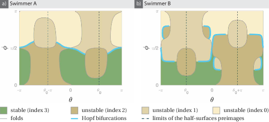
The level sets of and are shown in figure 1 for the helical swimmer A described in section 4 and shown in figure 6. Figure 1 can be used to find all the equilibria occurring for any given values of the experimental parameters. The arrows indicating increasing values of are valid on the upper border of the figure. The bold curves highlight the particular level sets corresponding to and . For these parameter values, the full and dashed lines have 8 intersections corresponding to 8 different relative equilibria at these values of the parameters. Once the pair () is found for a particular equilibrium, the orientation of the body can be inferred by computing and from (27) and (28). Note that this map also proves that there are relative equilibria for all orientations of (not all of them stable, more on this in section 3.3) but not for all orientations of : at equilibrium, the rotation axis is in a plane orthogonal to .
The maximal for which a given swimmer has any relative equilibria is equal to the largest singular value of the matrix (see equation (29a)). It is straightforward to show that for a swimmer of a given shape, the maximal value of is obtained by magnetising the body in a direction perpendicular to the "easy rotation axis" – i.e. perpendicular to the eigenvector of corresponding to its largest eigenvalue.
Finally, note that by definition (27), all functions of can be extended to the real line by imposing periodicity modulo . In particular, it will help to wrap figure 1 on a cylinder by identifying the borders at .

3.2 Symmetry of the rotational dynamic
The solutions of the ODE (23) come in symmetric pairs. Indeed, if the function is a solution, then so is
With obvious notations, one finds that in the body frame , , and .
In the magnetic frame, the equations of motion are autonomous. At any instant, if the body is oriented according to (w.r.t. the magnetic frame) and has angular velocity with respect to the magnetic frame, then the symmetric solution is rotated by through the axis perpendicular to both and and the angular velocity is the reflection of through the plane containing both and .
At relative equilibria, the body is locked in the magnetic frame () and symmetric solutions are obtained by rotations through with respect to the axis perpendicular to both and . Accordingly, one finds
| (30) |
The corresponding symmetry of figure 1 consists in a reflection through the line at followed by a horizontal translation by (making use of the -periodicity).
3.3 Stability
The linear stability of relative equilibria of (20) is given by the sign of the real part of the eigenvalues of the linearised dynamics matrix
| (31) |
where and are taken at that equilibrium. They are therefore explicit functions of and . Each equilibrium is thus associated with an index defined as the number of eigenvalues of with strictly negative real parts (counting multiplicities). An equilibrium is therefore unstable whenever its index is strictly less than . If the index is 3, it is stable (see figure 2).
We remark that the linearised dynamics matrices of symmetric pairs of relative equilibria (in the sense of section 3.2) have opposite eigenvalues. So if one equilibrium of the pair is stable, then the other is necessarily unstable with index 0.
As we move on the set of relative equilibria, stability changes only at bifurcation points of the dynamical system (23) (Kuznetsov, 2004). In this system almost all bifurcations are either folds or Hopf bifurcations.
 \phantomsubcaption\phantomsubcaption
3.3.1 Folds
Fold points are generically points where one real eigenvalue of is , so . At a fold, the linearised system admits a line of equilibria. This occurs when the parameterisation of the plane by looses regularity, that is when the Jacobian
| (32) |
vanishes. This condition makes them easy to track since we have the explicit parameterisation (29).
Finally, folds also correspond to the values of the experimental parameters and for which the number of equilibria changes. Therefore folds occur when the level sets of and in figure 1 are tangent333For fixed values of and , points of tangency of the level curves go by pair because of the symmetry described in section 3.2..
3.3.2 Hopf Bifurcations
Hopf bifurcations are points where has a pair of purely imaginary conjugate eigenvalues . Accordingly, relative equilibria on both sides of the Hopf bifurcation have indices differing by .
To find the Hopf bifurcations of (23), we apply the technique described in Kuznetsov (2004) and compute the bialternate product
| (33) |
where is the identity matrix in and are the elements of . By construction, the eigenvalues of are the three sums of pairs of eigenvalues of . The Hopf bifurcations are therefore obtained as the zero-level curve of . Note that also cancels when has two opposite real eigenvalues; these are removed in post-processing.
Hopf bifurcations also give rise to branches of periodic orbits. We used numerical continuation techniques to explore them and the results are exposed in section 4.3.
3.4 Translational trajectories corresponding to specific relative equilibria
By definition, the trajectory corresponding to a relative equilibrium has constant linear and angular velocities and in the body frame and is therefore helical. The axis of the helix is given by while its pitch and radius are given by (Crenshaw, 1993).
| (34) |
Substituting the equilibrium condition (25) in the equation for the outer layer behaviour (21) yields
| (35) |
Further substituting (35) in (34), we obtain
The swimmer evolves along a helix the axis of which is parallel to the axis of rotation of the external field (see eq. (35)). The so called chirality matrix is studied in details in Morozov et al. (2017) including a discussion of how the off-diagonal terms of Ch allow some non-chiral objects to nevertheless transform their rotational dynamic into translational motion.
3.4.1 Optimal and for maximal axial velocity of a magnetic swimmer
 \phantomsubcaption\phantomsubcaption
The axial velocity is the component of the velocity along the axis of rotation of the magnetic field:
| (36) |
Substituting the parametrisation (27, 29) to express and in terms of and allows to find the maximal axial velocity admissible for relative equilibrium trajectories as
| (37) |
3.4.2 Optimal magnetisation for large axial velocity
To optimally magnetise a swimmer of a given shape to achieve maximal axial velocity, we make use of to obtain
Noting that for some unit vector , we consider the expression
| (38) |
Let be the absolute maximizer of
| (39) |
over the unit vectors.
Next, we show that optimal magnetisation is achieved by picking orthogonal to . Note that while it is clear that (38) is optimised by picking and , at this point, is an upper bound on the maximal axial velocity of a swimmer of a given shape. We still need to show that there exists a such that . To this intent, remember from the previous section that for a given magnetisation, optimal axial velocity is indeed obtained at . In this case, by varying , we can pick to be any unit vector that is perpendicular to . In particular, it is possible to choose such that : the optimal velocity is reached for those values of .
Note that we are left with a one parameter family of magnetisations for which it is possible to find an equilibrium with . This degree of freedom may be used to try to bring the optimal equilibrium close to the stable region ( is itself expected to be neutrally stable at best).
Let parametrise the unit circle in the plane as . For each , compute the eigenvalues of the matrix (31)
Look for such that has a pair of purely imaginary eigenvalues. If such an exists, set the swimmer’s magnetic moment direction as . Then the two equilibria maximise the axial velocity with parameter values and , and at least one of them has stable relative equilibria in its neighbourhood.
Indeed the two pairs are then Hopf bifurcations of the system, and their respective stability matrices are opposite. So the unique real eigenvalue of one of the stability matrix is non-positive, while the pair of purely imaginary eigenvalues have zero real part. Therefore, at least one of these two Hopf bifurcation has stable relative equilibria in its neighbourhood.
An example where is chosen as to maximise the axial velocity on stable equilibria is presented in section 4.
3.5 There are almost always 0, 4, or 8 relative equilibria
 \phantomsubcaption\phantomsubcaption\phantomsubcaption\phantomsubcaption\phantomsubcaption\phantomsubcaption
We have seen is section 3.1 that the set of relative equilibria forms a 2-dimensional surface in the eight dimensional space . To visualise it we project it in by considering the function
| (40) |
and defining the surface as the image set of . Furthermore is extended to by asking that it be -periodic in .
The graph of , or equivalently the surface , is shown in figure 4 with the colour encoding the stability index (green is stable). Close inspection of equations (29) reveals that is not injective (see appendix B for details). One of the self-intersection of is found along the coordinate line with where for all . Furthermore, the two restrictions
| (41) | ||||
are symmetric in the sense of section 3.2: the symmetric equilibrium to a state in is in and vice-versa. This same symmetry also implies that has a mirror symmetry about the plane .
Because of the mirror symmetry between and , the number of relative equilibria for fixed parameters and is even. We now show that it is generically , , or . Using (29a) to express in terms of and , and substituting in (29b), we find
For fixed values of the parameters and , this is a trigonometric polynomial of degree 4 in ; it has therefore at most 8 roots (Powell, 1981).
does not have boundaries. Indeed, the mapping is continuous, and therefore any boundary would arise on the borders of the chart . However has no boundary at : for all , we have , and for fixed in , the curve is closed. Furthermore, has no boundary at : for , equation (29a) yields , so that for , the closed curve is reduced to the segment travelled twice, thereby sealing the boundaries at . By symmetry, does not have boundaries either.
Looking for relative equilibria for fixed parameter values and is equivalent to looking for intersections between and the straight line in -space with and . Since has no boundaries, slicing at gives a closed curve in the -plane. The straight line intersects this curve twice, except at folds or self-intersections of the curve. Since each relative equilibrium is uniquely parametrised by in the chosen intervals by equations (27, 28), self-intersections still count for two distinct relative equilibria. This eventually implies that the parameter space is cut by folds into regions with either 0, 4, or 8 corresponding equilibria (cf. fig. 4-4).
Further geometric properties of surface are studied in appendix B.
3.6 Experimental regimes diagram
 \phantomsubcaption\phantomsubcaption
Projecting the surface on the plane, and keeping track of the number of sheets projected on any given point, we obtain a diagram on which one can read of the number of equilibria (see figures 4 and 5). The general shape of this diagram is consistent across different swimmers: we found at most five different regimes that cover various regions of the plane. These regions vary in shape and sizes with the shape and magnetisation of a swimmer. However, their general arrangement is consistent as well as their broad features. For instance, the triangular region of the regime 2/8 (standing for 8 equilibria, 2 of which are stable) remains triangular even though it can be of very different proportions for different swimmers. The notable exception is the regime 0/4 present on the wings at large for swimmer B and absent for swimmer A. Some swimmers have it and some don’t. When that regime exists, we always found it at similarly large .
4 Helical swimmers and how to operate them
 \phantomsubcaption\phantomsubcaption
As stated in the introduction, the principal application motivating our study is the motion of rigid, helical and magnetic microswimmers. We therefore focus on two examples the bodies of which are helical rods with a circular cross-section, capped with half-spheres at the two ends: the swimmers A and B shown in fig. 6. We analyse many more examples in Rüegg-Reymond (2019). To compute the drag matrices of these helices, we use a code presented in Gonzalez (2009); Li and Gonzalez (2013); Gonzalez and Li (2015) and provided to us by the authors. The outer surface of the helical rod is discretised by one quadrature point in each patch defined by the mesh shown in fig. 6. The direction of the magnetic moment is chosen so that it is not aligned with the helix central axis. Lengths are scaled using the radius of gyration as the characteristic length . The numerical data for and corresponding to our examples can be found in appendix A.
4.1 Experimental regimes diagrams
The experimental parameters diagrams of both swimmers are shown in figure 5. We find 4 regions of parameters exhibiting relative equilibria. It is worth noting that there exist relative equilibria for a much wider range of experimental parameters for swimmer B than for swimmer A, with ranging from to and up to compared to and for swimmer A. The different range of mason numbers is readily understood by the analysis of section 3.1: the maximal Mason admitting a relative equilibrium is given by which is much larger for swimmer B than for swimmer A. Note that this is a property of the matrix and not of the chirality matrix. We do not have an analytical understanding of the range of .
Moreover the regimes diagram 5 that corresponds to the longer helix is more symmetric about the axis than that of the shorter helix 5. It is actually not exactly symmetric. We conjecture that for long helices the diagram will be very close to symmetric regardless of the direction of magnetic moment .
The other major difference between both diagrams is that swimmer B admits a regime for which relative equilibria exist but are all unstable (regime 0/4). The parameter regions corresponding to this regime are located at the extremal tips of the set of equilibria and are bounded by curves of Hopf bifurcations that have no counterparts for swimmer A.
Finally, remembering from section 3.6 that these diagrams are obtained by projecting the three-dimensional surfaces, we also include the corresponding surface from swimmer B in figure 19 in the appendix B. Note that for both swimmers, all the stable equilibria are bound to the region , in accordance with the intuition that the magnetic moment tries to align with the magnetic field .
Although these diagrams are useful to predict maximal Mason before step-out as well as the number of possible behaviours at given and , they also suggest a number of interesting questions. What happens when the system is multistable? How does the system behave when there are 4 equilibria but none of them are stable? In the simpler case where there exists a single stable equilibrium, are we sure that the system will always collapse to it? How to optimally handle the swimmer to get it where we want it to go?
To address these questions, we will both apply the techniques developed in section 3 and perform numerical experiments.
4.2 Numerical conditioning and quaternion formulation
We first cast (23) in a form that both allows for easier numerical integration and enables numerical continuations e.g. follow branches of periodic solutions sprouting from Hopf bifurcations as described in section 3.3.2.
Since the unknown in (23) is a rotation matrix, numerical treatment of the system can be eased by using a parametrisation of the group of rotations. Here we parameterise by quaternions which can be treated as 4-vectors by numerical integrators. The quaternion formulation of (23) is (Dichmann et al., 1996)
| (42) |
where
and , with
| (43) |
and , given as in (21). This parametersiation of rotations by quaternions is independent of the norm of the quaternion. Accordingly, the Jacobian of the right-hand side of (42) is singular, and this poses a problem for numerical continuation. To circumvent this issue, we use the modified system
| (44) |
This modified system ensures that the solutions are unit quaternions and the stability is the same as for the original system, both for steady states and periodic solutions.
4.3 Periodic solutions
 \phantomsubcaption\phantomsubcaption
Because the system displays Hopf bifurcation, we expect that it has periodic orbits for some regions of the experimental parameters and . We tracked these solutions with the Matlab package MatCont (Dhooge et al., 2008) applied to the ODE (44). The stability index of these periodic orbits is obtained from the Floquet multipliers (Kuznetsov, 2004) which are part of the code output. The starting points for continuations are chosen on the curves of Hopf bifurcations (drawn in blue in all figures). Each point on those curves is associated with a period depending on the purely imaginary eigenvalue of the stability matrix at that point. Then we chose to continue by finding the and that keep the period of the periodic orbit constant. By this process, each point on the curves of Hopf bifurcation gives rise to a curve of periodic orbits in the plane. We found that these curves both start and end at Hopf bifurcations. Gathering these curves of periodic orbits into a set forms a sheet of periodic orbits as shown in red (if unstable) and green (if stable) in figure 7. These sheets are obtained by interpolation of the darker lines, which represent branches obtained by numerical continuation of system (44) with period kept constant.
Note that at the beginning of this process, each point along a curve of Hopf bifurcations is associated with a period. In our system, all curves of Hopf bifurcations were found to begin and end at folds. This implies that the associated period goes to infinity making accurate numerical continuations difficult in the vicinity of these points. This is why the foils shown in figure 7 are incomplete.
For both swimmers A and B, the foil originating from the Hopf curve bordering the 2/4 regime seems to fill the very domain of that regime (we could not have a definite answer because of the numerical issue mentioned above). In our examples, all periodic solutions existing for regime 2/4 are unstable.
For swimmer B, the foil originating from the Hopf curve bordering the 0/4 regime seems to fill the domain of that regime but it is not limited to it. We note that some of these periodic orbits are stable and some are unstable. It is noteworthy that this foil is not restricted to the 0/4 regime as some of the unstable branches extend into the 1/4 regime.
There also exist other types of stable periodic orbits that do not connect to Hopf bifurcations. In particular, we study stable periodic orbits in regions which are well away in the 0/0 region and in the , and limits in a separate paper (Rüegg-Reymond and Lessinnes, 2018). These results are also described in the thesis of Rüegg-Reymond (2019).
In conclusion, as long as we stay in the regimes where there exist stable equilibria and well away from large , we systematically observed that all periodic orbits were unstable.
 \phantomsubcaption\phantomsubcaption
4.4 Phase portrait and basins of attraction
For both swimmers A and B, we study phase portraits of the dynamical system (42) obtained by integrating it numerically with many initial conditions for various parameter values . Showing quaternion dynamic is not geometrically straightforward as we have to project a four-dimensional dynamic onto a 2D sheet. The matter is simplified by the fact that the parameterisation 43 is independent of the norm of the quaternion: we can therefore drop one degree of freedom. The unit quaternions are represented in 3D by their three vector components , , and , and since opposed quaternions represent the same rotation, we have the convention that the scalar part . This representation is the 4D equivalent of representing the upper hemisphere of the sphere by flattening it onto the unit disc. Due to the equivalence of opposite quaternions, antipodal points on the outer boundary are equivalent. The phase portraits displayed in figure 8 show the vector part of the quaternions so that the dynamic is actually a dynamic in the unit ball.
Regime 1/4 is the only observed regime for which there is a unique stable steady state. We observed two different behaviours with numerical experiments in this regime. In most cases, there is no other stable special solution, and all trajectories obtained by numerical integration of (44) reach the stable steady state after some time, suggesting that it is globally attractive. For some swimmers, a stable periodic orbit coexists with a stable steady state for parameter regime 1/4. Each stable solution then has its own attraction basin. This second behaviour is studied in more detail in (Rüegg-Reymond, 2019).
In figure 8, we look closely at two particular examples of phase portraits for parameter values corresponding to cases where there are two stable relative equilibria: we picked a 2/8 regime for swimmer A ( and ) and a 2/4 regime for swimmer B ( and ). In both cases, all trajectories were found to tend to one or the other stable relative equilibrium which indicates that the union of their basins of attraction is likely to cover almost all of the possible initial orientations. Note that the trajectories are coloured according to the equilibrium that is reached so the blue and red shapes effectively draw out these basins of attraction. In regime 2/8 for swimmer A (fig. 8) we can observe that the two relative equilibria lie on two different accumulations of lines prefiguring the existence of two heteroclinic orbits, each linking together four relative equilibria. In regime 2/4 for swimmer B (fig. 8) the four relative equilibria coexist with two unstable periodic orbits found by numerical continuation from Hopf bifurcations (cf. section 4.3).
4.5 Optimising the magnetisation
Following the procedure described in section 3.4.2, we look for a magnetisation direction that maximises the axial velocity over relative equilibria for swimmers with the same shapes as the helical swimmers A and B (cf. fig. 6). Results are summarised in table 1. The optimal magnetic moment direction is given with respect to the basis described in appendix A – the third director is aligned with the helix axis. Axial velocities as functions of for various values of of the optimally magnetised versions of swimmers A and B are shown in figure 9.
| Swimmer geometry | Experimental parameters | |||
|---|---|---|---|---|
| (rad) | ||||
| Similar to swimmer A | 0.0333 | 1.5708 | ||
| Similar to swimmer B | 0.9880 | 1.5708 | ||
 \phantomsubcaption\phantomsubcaption
4.6 How to operate bistable swimmers?
We observe that for arbitrary magnetisations, optimal experimental parameters are typically found in the bistable regime. Furthermore, we provided examples in section 4.4 for which the basins of attraction of the two stable relative equilibria (almost) fill the full phase space. In practice, it would therefore not do to simply switch on the external field at the optimal and . Indeed by doing so, one would sometimes reach the optimal regime and sometimes reach the other stable equilibrium. Here we discuss how to systematically bring the swimmer in one chosen relative equilibrium.
We present two strategies shown in figure 10. In all cases, they should work without requiring detailed knowledge of the particular swimmer. The first strategy is to use the fact that the region of stability of the two equilibria are in most cases different. Hence, a simple try is to keep constant and to change slowly until the current branch is destabilised. Then, we can slowly bring back to its original value: if no further jump is observed then the swimmer is now at the (only) other equilibrium – see the panel 10) in figure 10.
The other strategy is based on the following observations. First, in all examples presented here and in Rüegg-Reymond (2019), we found that the stable region of the plane is simply connected (when accounting for the -periodicity in ). This means that it must be possible to smoothly transform any stable equilibrium in another equilibrium by smoothly changing and or equivalently by smoothly changing and . Next, direct inspection of (29) shows that one can qualitatively understand the transition from one to two stable equilibria by considering the low and limits (keeping in mind that stable equilibria are found only for . In the first case, is small and the first term dominates in (29b): there is a two-to-one relation from to . But in the second case, is large and the second term dominates in (29b): there is a four-to-one relation from to . In practice, we have systematically observed that only one of the two equilibria at is ever stable and that two of the equilibria at are stable.
Therefore, at low , we have low444That is because the second factor in (29a) is bounded from below by (the smaller non-vanishing singular value of ). Hence . and in that region, there is a one-to-one relation between and the unique stable equilibria existing at that value of555Note that the range can be very narrow for some swimmers and fairly broad for others. For example, for swimmer we have while for swimmer B we have . That is for swimmer A, equilibria will be found at low provided that deviates from by no more than . While for swimmer B, can deviate from by up to . .
The second strategy is therefore as follows (see also panels 10-10) of figure 10):
-
Step 1 :
Study the swimmer at low . Starting at which is always stable, slowly increase up to the loss of stability: this defines the boundary of the interval above.
-
Step 2 :
Bring well on one side of the interval (there is no need to be on the boundary).
-
Step 3 :
Slowly increase , then optimise and by trial and errors. Note the optimal values and . At this stage there is no guarantee that we are at the optimal equilibrium: the other stable one might be better.
-
Step 4 :
Slowly bring back to zero and then slowly decrease back to small values.
-
Step 5 :
Set to the other side of (as compared to the choice made at step 1).
-
Step 6 :
Slowly increase back to , then slowly bring back to and compare the axial velocity obtained in this final state to that which was obtained at step 3.
-
Step 7 :
If the last axial velocity is greatest then locally optimise and again and you found the optimum. If the axial velocity of step 4 was higher, then come back to that state by following backward the sequence 4 to 6.
 \phantomsubcaption\phantomsubcaption\phantomsubcaption
5 Axial velocity of the three beads cluster
 \phantomsubcaption\phantomsubcaption
 \phantomsubcaption\phantomsubcaption
Many studies report experimentally and/or numerically on the dependance of the axial velocity (up to scaling choices) on the Mason number (up to scaling choices) at constant angle between the external field and its axis of rotation. The parameterisations of the axial velocity (37) and of and (29) proposed here provide an analytical expression of that relation. Indeed, the curve is recovered by looking up the values of and along a level curve of the function . In this section, we use this new tool to revisit swimmers that were used as examples in Meshkati and Fu (2014) and in Morozov et al. (2017). It consists in three contiguous spherical beads arranged so that the lines joining their centres form a angle.
To compute, we rescale the mobility matrices provided in the original studies as described section 2.2. The resulting non-dimensional matrices are listed in appendix A. Our results are gathered in figures 11 and 13, where we systematically provide two sets of axes: all the starred quantities correspond to the scaling choices of the original authors while the plain ones are as defined in the present document. A bold line indicates the presence of a branch of stable equilibria, while a thin line shows unstable equilibria. To understand the number of equilibria in the system, it is important to note that the axial velocity of an equilibrium and of its symmetric twin (in the sense of section 3.2) are equal (see equation (36) together with the fact that at equilibria, ). Hence every point on these plots correspond to a pair of equilibria. As already mentioned at most one equilibrium of a symmetric pair can be stable.
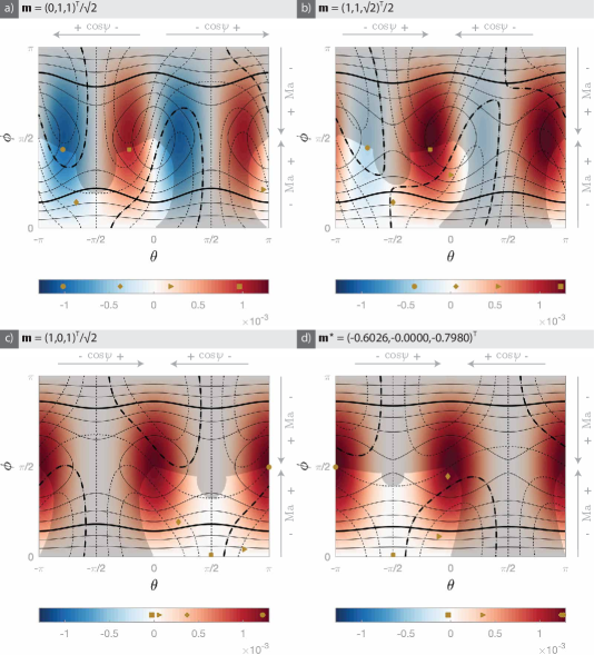
Figures 12 and 14 show the corresponding experimental regime diagrams from which one can readily read the number of (stable) equilibria for any pairs of experimental parameters values of and , while figures 12 and 15 display the -plane with axial velocity and level curves of and .
Generally, Morozov et al. (2017) studied the axial velocity as a function of the shape and magnetisation of the swimmer. In particular, they showed that for the same geometry, different magnetisation orientation can produce vastly different responses: for some, increasing the Mason number provokes a linear increase of the swimmer’s velocity (e.g. the curve replicated on fig. 13), while for others, the response is not linear (e.g. the curve replicated on fig. 13, see also Fu et al. (2015)). The authors also discussed the optimisation of both the shape and the magnetisation in some specific cases. However their analysis was focused on the case of . It turns out that faster axial motion can be achieved by relaxing the constraint.
 \phantomsubcaption\phantomsubcaption\phantomsubcaption\phantomsubcaption
 \phantomsubcaption\phantomsubcaption\phantomsubcaption\phantomsubcaption
 \phantomsubcaption\phantomsubcaption\phantomsubcaption\phantomsubcaption
Meshkati and Fu (2014) are to our knowledge the only other authors studying cases with . They obtained an algebraic system of equations for the relative equilibria equivalent to our (25) and proceeded to solve it numerically. Interestingly, they reported gaps in the curves which they attributed to numerical issues with their root finding algorithm. The present study indicates that the branch of equilibria does exist but that these equilibria are actually unstable precisely in the gaps where their algorithm failed. Hence the axial velocities in those gaps are not achievable in actual experiments.
The axial velocities obtained with the mobility matrix computed by Meshkati and Fu (2014, 2017) are shown in figure 11 in a way that can be straightforwardly compared with figure 11 of Meshkati and Fu (2014). We keep their characteristic length , chosen as the distance between the two furthest bead centres, expressed in terms of the radius of one bead as . Because the authors used the inverse axial velocity of the magnetic field as a characteristic timescale, their non-dimensional axial velocity is proportional to our pitch . There is also a sign difference between their axial velocity and our pitch . It might be due to different sign conventions, but we have not been able to pinpoint the exact cause. Both scales are shown on fig. 11 to make comparison with their figure 11 easier. Note that the dimensional axial velocity of the swimmer can be recovered from our non-dimensional axial velocity as , and from their non-dimensional axial velocity as , while the dimensional trajectory pitch is recovered from the non-dimensional trajectory pitch as .
Morozov et al. (2017) report using the same algorithm as Meshkati and Fu (2014) to compute the mobility matrix of the three bead swimmer, without explicitly presenting their result. To compare our results, we transformed the mobility matrix given by Meshkati and Fu (2014) according to the conventions of Morozov et al. (2017) (cf. appendix A. We report the corresponding axial velocities in figure 13 for a few choices of magnetisation. This figure is to be compared with figures 7 and 9 of Morozov et al. (2017). To make comparison straightforward, we indicated both the scales we use, and the scales they chose. The dimensional axial velocity can be recovered from our non-dimensional velocity as , where , with the radius of one bead, or from their non-dimensional axial velocity as , where and are defined as in appendix A. The dimensional angular velocity of the magnetic field is recovered from their non-dimensional axial velocity as – note it can also be computed from the Mason number using formula 12.
It is well worth noting that for a given magnetisation, the optimal axial velocities are often obtained for values of well away from . In particular, for (fig. 13), the extremal non-dimensional axial velocities, which are obtained for and , are 26% larger (in absolute value) than the extremal axial velocities reached with the constraint . Similarly, for (fig. 13), the maximal non-dimensional axial velocity, reached with and , is 13% larger than the maximal axial velocity reached with . The last panel of figure 13 showcases the optimal magnetisation obtained by our method of section 3.4.2.
 \phantomsubcaption\phantomsubcaption
 \phantomsubcaption\phantomsubcaption
Morozov et al. (2017) also investigated how to optimise the axial velocity by varying the shape of swimmers. In particular, they studied three beads clusters with different vertex angles between the lines joining their centres, and found that the axial velocity is optimised for a vertex angle of . Using the mobility matrix they reported for this optimal swimmer (cf. appendix A), we show in figure 16 the axial velocity as a function of the Mason number at different values of for two distinct magnetisation directions: , and the optimal magnetisation direction . Note that the largest axial velocity is reached for with the optimal magnetisation direction, but an axial velocity only 2% smaller is reached with for the non optimal magnetisation direction . The corresponding experimental regimes diagram are provided in figure 17, and figure 18 shows the axial velocity and level sets of and as functions of the mapping parameters and .
 \phantomsubcaption\phantomsubcaption
6 Conclusions
For all examples presented here, we did observe that when the magnetisation is optimal, the optimal angle between the external field and its rotation axis was indeed . In that case, we also observed a linear relation between the axial velocity and the Mason number (which linearly parameterises the angular velocity of the external field) over the range of Mason numbers on which the swimmer is bistable: the optimal equilibrium being reached just before step-out. Note that we do not know of a proof of this feature as a general result.
However, it is practically difficult to accurately control the magnetisation direction. For arbitrary magnetisation directions, optimal driving parameters were often found both well away from step-out and well away from . In those cases, the relation between and is strongly nonlinear. The good news however is that the optimal axial velocities achieved for all magnetisations were comparable in order of magnitude to those obtained with optimal magnetisation. The conclusion is therefore that in practice, we do not have to magnetise the swimmer optimally provided that we learn how to pinpoint optimal and .
Furthermore, optimal driving parameters were always found in a bistable regime. It would be very interesting to have an experimental verification of the practicality of the methods proposed here for systematically reaching the faster equilibrium.
Note that we have studied a non-dimensional version of the axial velocity. By plugging the dimensions back in, it is straightforward to show that the dimensional axial velocity is proportional to the angular velocity of the external field (and not to ). Therefore, in practice, given a stable equilibrium, we can always multiply the axial velocity by a factor by increasing both and the magnitude of the external field the same factor . By doing so, we stay on the exact same non-dimensional equilibrium.
Finally, the mobility matrix of a given experimental swimmer and its magnetisation are not easy to measure in practice. We believe that an interesting line of enquiry would be to make use of the formal parameterisation of the equilibria proposed here to reverse engineer the broad features of the experimental parameters diagram. One could for instance infer the outer boundary of the region of existence of stable equilibria by tracking and at step-out. It should then be possible to recover interesting informations about the matrix of the swimmer a posteriori. Note for instance that can be directly inferred from the maximal mason number for which there exists an equilibrium. The shape of the curve could also be used to infer properties of . Once these are known, the methods of section 3 can be used to infer optimal driving parameters of this particular swimmer.
Acknowledgements
We thank Oscar Gonzalez for providing the code used for computing the drag matrices, and John H. Maddocks for his support. This work was funded by the Swiss National Science Foundation (SNF) project number 200021-156403.
Declaration of interest. The authors report no conflict of interest.
 \phantomsubcaption\phantomsubcaption\phantomsubcaption\phantomsubcaption\phantomsubcaption\phantomsubcaption
Appendix A Numerical Data of Examples
In section 4, swimmers A and B are helical rods with geometry and magnetisation directions as specified in table 2. The magnetisation directions are given in the basis in which the helical centreline of the rod is parametrised as
where , is the helix radius, and is the helix pitch, so that the third basis direction corresponds to the helix axis. The total arc-length listed in table 2 is the length of the helical centreline of the rod, and this rod is additionally capped by two half spheres with the same radius as the cross-section (cf. fig. 6).
| Helical swimmer | helix radius | helix pitch | total arc-length | cross-section radius | magnetisation direction () |
|---|---|---|---|---|---|
| Swimmer A | |||||
| Swimmer B |
The drag matrices obtained from this information using Gonzalez’ code (Gonzalez, 2009; Li and Gonzalez, 2013; Gonzalez and Li, 2015) are respectively
| and | |||
Since these results are not exactly symmetric, we correct this by using in our computations. Relevant material parameters are listed in table 3.
| Swimmer | (rad) | ||||||
|---|---|---|---|---|---|---|---|
| Swimmer A | 0.0333 | 0.0241 | -0.0027 | 0.0091 | -1.3871 | ||
| Swimmer B | 0.9244 | 0.0497 | 0.3243 | 0.8160 | -1.5680 | ||
| Meshkati and Fu (2014) | 0.1858 | 0.1274 | -0.0377 | 0.0095 | -0.0012 | 0.0549 | 1.2170 |
| Morozov et al. (2017) | |||||||
| Vertex angle: 90∘ | |||||||
| 0.1761 | 0.1190 | 0.0363 | 0.0533 | 1.5708 | |||
| 0.1735 | 0.1271 | 0.0397 | -0.0105 | -0.0014 | 0.0422 | 1.2253 | |
| 0.1698 | 0.1360 | 0.0448 | -0.0278 | -1.5708 | |||
| 0.1575 | 0.1360 | -0.0431 | -0.0156 | 1.5708 | |||
| Vertex angle: 122.7∘ | |||||||
| 0.2177 | 0.1148 | 0.0853 | -0.0026 | 0.0854 | 1.5122 | ||
| 0.1792 | 0.1172 | -0.0779 | -0.0442 | 1.5708 |
Three beads cluster with a vertex angle of 90∘ (taken from Meshkati and Fu (2014) and scaled taking m ( is the radius of one bead) and assuming that the fluid viscosity is Pa s):
Appendix B More on the Geometry of the Surface of Equilibria
 \phantomsubcaption\phantomsubcaption\phantomsubcaption
In order to better understand the geometry of the surface described in section 3.1, we give here a detailed account of all its self-intersections. The surface is parametrised by variables and . In section 3.5 we indicated the self-intersection at , where depends only on the swimmer, and used it to split the surface into two symmetric halves and . Upon close inspection of the parametrisation (29) we find that the self-intersections of are given by
| (45a) | |||||
| (45b) | |||||
| (45c) | |||||
| (45d) | |||||
We can see by comparing the different panels of figures 4 and 19 that the two halves and intersect each other at multiple locations. A crucial question to understand the visualisation is whether there are self-intersections within the same half. We can readily see that there are on fig. 4. Intersection (45c) defines the splitting between and while (45d) is necessarily an intersection between the two halves by definition of and . Therefore self-intersections within the same half are either in the family (45a) or (45b).
 \phantomsubcaption\phantomsubcaption\phantomsubcaption
Figure 20 shows all the self-intersections of the surface for swimmer A. On figure 20, the type (45a) intersection curve is symmetric about and , while the type (45b) intersection curve is symmetric about . Two points of either intersection curve in the -plane coincide on if they have the same height . This results in self-intersections within the same half-surface if those two points lie within the same region of the -plane delimited by the and vertical lines (taking -periodicity of the parametrisation into account), and in intersections between and otherwise.
Self-intersections of type (45a) of a half-surface occur when is such that : the closer is to or , the smaller the set of such . Type (45b) self-intersections of arise for such that : the closer is to , the smaller the set of such . For swimmer A, is quite close to (cf fig. 20); therefore type (45b) self-intersections within the same half are indiscernible on figure 20-20). A larger set of satisfy the condition for type (45a) self-intersections to occur within the same half .
Knowing how the surface self-intersects helps understanding how the half surfaces and join, and how the stability index is continuous across the two halves. We illustrate this by showing curves obtained as sections of at constant values of for swimmer A in fig. 21.
References
- Bell et al. [2007] D. J. Bell, S. Leutenegger, K. M. Hammar, L. X. Dong, and B. J. Nelson. Flagella-like Propulsion for Microrobots Using a Nanocoil and a Rotating Electromagnetic Field. In Proceedings 2007 IEEE International Conference on Robotics and Automation, pages 1128–1133, Apr. 2007. doi: 10.1109/ROBOT.2007.363136.
- Bente et al. [2018] K. Bente, A. Codutti, F. Bachmann, and D. Faivre. Biohybrid and Bioinspired Magnetic Microswimmers. Small, 14(29):1704374, July 2018. ISSN 1613-6829. doi: 10.1002/smll.201704374.
- Crenshaw [1993] H. C. Crenshaw. Orientation by Helical Motion–I. Kinematics of the Helical Motion of Organisms with up to six Degrees of Freedom. Bulletin of Mathematical Biology, 55(1):197–212, 1993.
- Dhooge et al. [2008] A. Dhooge, W. Govaerts, Y. A. Kuznetsov, H. G. E. Meijer, and B. Sautois. New features of the software MatCont for bifurcation analysis of dynamical systems. Mathematical and Computer Modelling of Dynamical Systems, 14(2):147–175, Apr. 2008. ISSN 1387-3954. doi: 10.1080/13873950701742754.
- Dichmann et al. [1996] D. J. Dichmann, Y. Li, and J. H. Maddocks. Hamiltonian Formulations and Symmetries in Rod Mechanics. Mathematical Approaches to Biomolecular Structure and Dynamics, IMA Volumes in Mathematics and Its Applications, 82:71–113, 1996.
- Dreyfus et al. [2005] R. Dreyfus, J. Baudry, M. L. Roper, M. Fermigier, H. A. Stone, and J. Bibette. Microscopic artificial swimmers. Nature, 437(7060):862–865, Oct. 2005. ISSN 1476-4687. doi: 10.1038/nature04090.
- Ebbens and Howse [2010] S. J. Ebbens and J. R. Howse. In pursuit of propulsion at the nanoscale. Soft Matter, 6(4):726–738, 2010. doi: 10.1039/B918598D.
- Felfoul et al. [2016] O. Felfoul, M. Mohammadi, S. Taherkhani, D. de Lanauze, Y. Z. Xu, D. Loghin, S. Essa, S. Jancik, D. Houle, M. Lafleur, L. Gaboury, M. Tabrizian, N. Kaou, M. Atkin, T. Vuong, G. Batist, N. Beauchemin, D. Radzioch, and S. Martel. Magneto-aerotactic bacteria deliver drug-containing nanoliposomes to tumour hypoxic regions. Nature Nanotechnology, 11(11):941–947, Nov. 2016. ISSN 1748-3395. doi: 10.1038/nnano.2016.137.
- Fu et al. [2015] H. C. Fu, M. Jabbarzadeh, and F. Meshkati. Magnetization directions and geometries of helical microswimmers for linear velocity-frequency response. Physical Review E, 91(4):1–13, 2015. doi: 10.1103/PhysRevE.91.043011.
- Gao and Wang [2014] W. Gao and J. Wang. The Environmental Impact of Micro/Nanomachines: A Review. ACS Nano, 8(4):3170–3180, Apr. 2014. ISSN 1936-0851. doi: 10.1021/nn500077a.
- Ghosh and Fischer [2009] A. Ghosh and P. Fischer. Controlled Propulsion of Artificial Magnetic Nanostructured Propellers. Nano Letters, 9(6):2243–5, June 2009. doi: 10.1021/nl900186w.
- Ghosh et al. [2012] A. Ghosh, D. Paria, H. J. Singh, P. L. Venugopalan, and A. Ghosh. Dynamical configurations and bistability of helical nanostructures under external torque. Physical Review E, 86(3), Sept. 2012. doi: 10.1103/PhysRevE.86.031401.
- Ghosh et al. [2013] A. Ghosh, P. Mandal, S. Karmakar, and A. Ghosh. Analytical theory and stability analysis of an elongated nanoscale object under external torque. Physical Chemistry Chemical Physics, 15(26):10817–10823, 2013. doi: 10.1039/C3CP50701G.
- Gonzalez [2009] O. Gonzalez. On stable, complete, and singularity-free boundary integral formulations of exterior Stokes flow. SIAM Journal on Applied Mathematics, 69(4):933–958, 2009.
- Gonzalez and Li [2015] O. Gonzalez and J. Li. A convergence theorem for a class of Nyström methods for weakly singular integral equations on surfaces in R3. Mathematics of Computation, 84(292):675–714, 2015.
- Gonzalez et al. [2004] O. Gonzalez, A. B. A. Graf, and J. H. Maddocks. Dynamics of a Rigid Body in a Stokes Fluid. Journal of Fluid Mechanics, 519:133–160, 2004.
- Happel and Brenner [1983] J. Happel and H. Brenner. Low Reynolds Number Hydrodynamics: With Special Applications to Particulate Media. Mechanics of Fluids and Transport Processes. Springer Netherlands, 1983. ISBN 978-90-247-2877-0.
- Hinch [1991] E. J. Hinch. Perturbation Methods. Cambridge University Press, 1991.
- Honda et al. [1996] T. Honda, K. I. Arai, and K. Ishiyama. Micro Swimming Mechanisms Propelled by External Magnetic Fields. IEEE Transactions on Magnetics, 32(5):5085–5087, 1996.
- Kim and Karrila [2013] S. Kim and S. J. Karrila. Microhydrodynamics: Principles and Selected Applications. Courier Corporation, 2013.
- Kuznetsov [2004] Y. A. Kuznetsov. Elements of Applied Bifurcation Theory. Number 112 in Applied Mathematical Sciences. Springer, New York, NY, 3. ed edition, 2004. ISBN 978-1-4419-1951-9. OCLC: 815949776.
- Li and Gonzalez [2013] J. Li and O. Gonzalez. Convergence and conditioning of a Nyström method for Stokes flow in exterior three-dimensional domains. Advances in Computational Mathematics, 39(1):143–174, 2013. doi: 10.1007/s10444-012-9272-1.
- Mahoney et al. [2014] A. W. Mahoney, N. D. Nelson, K. E. Peyer, B. J. Nelson, and J. J. Abbott. Behavior of rotating magnetic microrobots above the step-out frequency with application to control of multi-microrobot systems. Applied Physics Letters, 104(14):1–5, 2014. doi: 10.1063/1.4870768.
- Man and Lauga [2013] Y. Man and E. Lauga. The wobbling-to-swimming transition of rotated helices. Physics of Fluids, 25(7):071904, July 2013. ISSN 1070-6631. doi: 10.1063/1.4812637.
- Medina-Sánchez et al. [2016] M. Medina-Sánchez, L. Schwarz, A. K. Meyer, F. Hebenstreit, and O. G. Schmidt. Cellular Cargo Delivery: Toward Assisted Fertilization by Sperm-Carrying Micromotors. Nano Letters, 16(1):555–561, Jan. 2016. ISSN 1530-6984. doi: 10.1021/acs.nanolett.5b04221.
- Meshkati and Fu [2014] F. Meshkati and H. C. Fu. Modeling rigid magnetically rotated microswimmers: Rotation axes, bistability, and controllability. Physical Review E, 90(6):1–11, 2014. doi: 10.1103/PhysRevE.90.063006.
- Meshkati and Fu [2017] F. Meshkati and H. C. Fu. Erratum: Modeling rigid magnetically rotated microswimmers: Rotation axes, bistability, and controllability [Phys. Rev. E 90 , 063006 (2014)]. Physical Review E, 95(6), June 2017. ISSN 2470-0045, 2470-0053. doi: 10.1103/PhysRevE.95.069904.
- Morozov and Leshansky [2014] K. I. Morozov and A. M. Leshansky. The chiral magnetic nanomotors. Nanoscale, 6(3):1580–1588, 2014. doi: 10.1039/C3NR04853E.
- Morozov et al. [2017] K. I. Morozov, Y. Mirzae, O. Kenneth, and A. M. Leshansky. Dynamics of arbitrary shaped propellers driven by a rotating magnetic field. Physical Review Fluids, 2(4):044202, Apr. 2017. doi: 10.1103/PhysRevFluids.2.044202.
- Mushtaq et al. [2015] F. Mushtaq, M. Guerrero, M. S. Sakar, M. Hoop, A. M. Lindo, J. Sort, X. Chen, B. J. Nelson, E. Pellicer, and S. Pané. Magnetically driven Bi 2 O 3 /BiOCl-based hybrid microrobots for photocatalytic water remediation. Journal of Materials Chemistry A, 3(47):23670–23676, 2015. doi: 10.1039/C5TA05825B.
- Nelson et al. [2010] B. J. Nelson, I. K. Kaliakatsos, and J. J. Abbott. Microrobots for Minimally Invasive Medicine. Annual Review of Biomedical Engineering, 12:55–85, Aug. 2010. doi: 10.1146/annurev-bioeng-010510-103409.
- Peyer et al. [2013] K. E. Peyer, L. Zhang, and B. J. Nelson. Bio-Inspired Magnetic Swimming Microrobots for Biomedical Applications. Nanoscale, 5(4):1259–72, Feb. 2013. doi: 10.1039/c2nr32554c.
- Powell [1981] M. J. D. Powell. Approximation Theory and Methods. Cambridge University Press, 1981.
- Rüegg-Reymond [2019] P. Rüegg-Reymond. On the Dynamics of Magnetic Micro-Swimmers. PhD thesis, EPFL, 2019.
- Rüegg-Reymond and Lessinnes [2018] P. Rüegg-Reymond and T. Lessinnes. Asymptotic Dynamics of Magnetic Micro-Swimmers. arXiv:1807.09059, 2018.
- Tottori et al. [2012] S. Tottori, L. Zhang, F. Qiu, K. K. Krawczyk, A. Franco-Obregón, and B. J. Nelson. Magnetic helical micromachines: Fabrication, controlled swimming, and cargo transport. Advanced Materials, 24(6):811–816, Feb. 2012. doi: 10.1002/adma.201103818.
- Vach et al. [2015] P. J. Vach, P. Fratzl, S. Klumpp, and D. Faivre. Fast Magnetic Micropropellers with Random Shapes. Nano Letters, 15(10):7064–7070, Oct. 2015. ISSN 1530-6984. doi: 10.1021/acs.nanolett.5b03131.
- Yan et al. [2017] X. Yan, Q. Zhou, M. Vincent, Y. Deng, J. Yu, J. Xu, T. Xu, T. Tang, L. Bian, Y.-X. J. Wang, K. Kostarelos, and L. Zhang. Multifunctional biohybrid magnetite microrobots for imaging-guided therapy. Science Robotics, 2(12):eaaq1155, Nov. 2017. ISSN 2470-9476. doi: 10.1126/scirobotics.aaq1155.