Reinforcement Learning with Adaptive Curriculum Dynamics Randomization
for Fault-Tolerant Robot Control
Abstract
This study is aimed at addressing the problem of fault tolerance of quadruped robots to actuator failure, which is critical for robots operating in remote or extreme environments. In particular, an adaptive curriculum reinforcement learning algorithm with dynamics randomization (ACDR) is established. The ACDR algorithm can adaptively train a quadruped robot in random actuator failure conditions and formulate a single robust policy for fault-tolerant robot control. It is noted that the hard2easy curriculum is more effective than the easy2hard curriculum for quadruped robot locomotion. The ACDR algorithm can be used to build a robot system that does not require additional modules for detecting actuator failures and switching policies. Experimental results show that the ACDR algorithm outperforms conventional algorithms in terms of the average reward and walking distance.
I Introduction
Robots are being increasingly applied in a wide range of fields such as factory automation and disaster assessment and rescue. In the existing approaches, the control law for robots are manually defined. However, in the presence of significant uncertainties in operating environments, the control law and states to be considered may not be easily identifiable, rendering such manual description challenging. To address these issues, reinforcement learning has attracted attention as a promising method that can automatically establish the control law without a clear description of how to realize a task of interest. A reinforcement learning framework learns, by trial and error, a policy that maximizes the reward, which is a measure of the goodness of the behavior in a certain environment. To realize reinforcement learning, it is necessary to only specify a task to be performed and design an appropriate reward function for the task.
Notably, to implement reinforcement learning in the real world, trial and error processes must be performed in real time. However, this approach may pose safety risks for the robot and surrounding environment. To ensure safety and cost effectiveness, robots are often trained in simulation environments before being applied in real world (Sim2Real). Reinforcement learning in simulation environments has achieved human-level performance in terms of the Atari benchmark [1] and robot control [2, 3]. However, Sim2Real is often ineffective owing to the gap between the simulation and real world, named reality gap, which can be attributed to the differences in physical quantities such as friction and inaccurate physical modeling. A straightforward approach to solve this problem is system identification, in which mathematical models or computer simulators of dynamical systems are established via measured data. However, the development of a realistic simulator is extremely costly. Even if system identification can be realized, many real-world phenomena associated with failure, wear, and fluid dynamics cannot be reproduced by such simulators. A typical approach to bridge the reality gap is domain randomization [4]. Domain randomization randomizes the parameters of the simulators to expose a model of interest to various environments. The model is expected to learn a policy that is effective in various environments, thereby narrowing the reality gap. Domain randomization has been used to successfully apply Sim2Real for the visual servo control of robot arms [4, 5] and locomotion control of quadruped robots [6].

|

|
Notably, reinforcement learning involves certain limitations. Figure 1 shows that even though a quadruped robot can walk owing to reinforcement learning (top row), the robot may turn over owing to the actuator failure of one leg (bottom row). In this context, fault-tolerant control is critical for robots working in remote or extreme environments such as disaster sites [7] because such robots can often not be repaired onsite. Several researchers have focused on fault-tolerant robot control based on reinforcement learning [8, 9]. However, these studies assume that the robots can detect internal failures and switch their policies according to the failures. Such robots require an additional module for diagnosing internal failures along with a module for control. In this context, robot systems designed for detecting all possible failures may be prohibitively complex [10]. To address this aspect, in this study, we establish a reinforcement learning algorithm for fault-tolerant control of quadruped robots against actuator failure. In this framework, the control law can ensure the locomotion of quadruped robots even if several actuators in the robot legs fail. Furthermore, we develop a fault-tolerant control system that does not include any self-diagnostic modules for actuator failures. To this end, an adaptive curriculum dynamics randomization (ACDR) algorithm is proposed that can learn a single robust control policy against actuator failures by randomizing the dynamics of quadruped robots with actuator failures. In addition, we develop a curriculum learning algorithm that adaptively trains the quadruped robots to achieve an enhanced walking ability. It is noted that the hard2easy curriculum, in which the training is initiated in difficult conditions that progressively becomes easier, is more effective than an easy2hard curriculum, which is commonly used. Experiments are conducted to demonstrate the effectiveness of the ACDR algorithm in comparison with conventional algorithms.
The key contributions of this study can be summarized as follows:
-
•
We establish a reinforcement learning algorithm to address the problem of fault tolerance of quadruped robots to actuator failures and realize fault-tolerant control.
-
•
The ACDR algorithm to proposed effectively learn a single robust control policy against actuator failures. The ACDR algorithm does not require any self-diagnosis modules for detecting internal failures, which must be implemented in conventional systems.
-
•
We demonstrate that the ACDR algorithms outperform conventional algorithms in terms of the average reward and walking distance.
-
•
For fault-tolerance control of quadruped robots, we find that the hard2easy curriculum is effective than the easy2hard curriculum.
II Related work
Domain randomization [4, 11] is aimed at enhancing generalization performance of the policy identified in simulations. Domain randomization requires a prescribed set of dimensional simulation parameters, , to randomize and the corresponding sampling interval. The -th element of is sampled from the uniform distribution on the closed interval . Using a set of the parameters , we can realize robot learning in various simulation environments. This randomization is expected to bridge the reality gap between the simulation and real world. Tobin et al. [4] successfully applied Sim2Real for visual robot control by randomizing the visual rendering of the environments. Moreover, Sim2Real has been successfully applied to control a robot arm [5] and quadruped robot [6] by randomizing physical parameters such as the robot mass and floor friction coefficient. In particular, we refer to the physical parameter randomization [5, 6] as dynamics randomization, thereby distinguishing it from visual domain randomization [4]. To implement dynamics randomization, the interval must be carefully determined, as an inappropriate interval is likely to result in failure to learn [12], a policy with considerable variance [13], or a conservative policy [14].
For reinforcement learning, it is effective to start with an easy task in order to succeed in a difficult task. Curriculum learning [15] is a learning process in which the difficulty of a task is gradually increased during training. Curriculum learning is mainly applied in navigation [16] and pickup tasks involving robot arms[17]. Luo et al. [18] proposed a precision-based continuous curriculum learning (PCCL) strategy that adjusts the required accuracy in a sequential manner during learning for a robot arm and can accelerate learning and increase the task accuracy. In general, it is difficult to determine the appropriate level of difficulty of a task in curriculum learning. Consequently, approaches that adaptively adjust the difficulty level for the agent through the learning process are attracting attention. Wang et al. [19] proposed a paired open-ended trailblazer (POET) strategy, which ensures an appropriate level of difficulty by co-evolving the environment and policies, and enables walking in difficult terrain. Moreover, curriculum learning in which the randomization interval is adaptively varied can help realize domain randomization [13, 20]. Xie et al. [20] considered a stepping-stone walking task with constrained scaffolding. The authors estimated the agent performance on each grid of the random parameters and adaptively varied the difficulty by decreasing and increasing the probability of occurrence of grids with high and low performance values, respectively. This algorithm can enhance the performance and robustness of the model. In general, the design of the environment and curriculum considerably influence the performance of learning to work [21]. To realize natural walking behavior, it is necessary to limit the torque. To this end, a curriculum that starts with a higher value, such as x, in the early stages of learning and gradually reduces the torque to the target value is considered to be effective [14].
To realize fault-tolerant robot control, Yang et al. [8] considered the joint damage problem in manipulation and walking tasks. The authors established a method to model several possible fault states in advance and switch among them during training. When the system encountered a failure, the method increased the robustness against joint damage by switching the policy. Kume et al. [9] proposed a method for storing failure policies in a multidimensional discrete map in advance. When the robot recognized a failure, it retrieved and applied these policies, thereby exhibiting a certain adaptability to robot failure. Notably, the existing failure-aware learning methods assumed that the robot can recognize its damage state. It remains challenging to develop a system that can achieve high performance with a single policy regardless of whether the robot is in a normal or failed state, even if the robot does not recognize the exact damage state.
III Method
To realize fault-tolerant robot control without additional modules, we propose an ACDR algorithm for reinforcement learning. The objective is to formulate a single robust policy that can enable a robot to perform a walking task even if actuator failure occurs. We assume that the quadruped robot cannot recognize its damage state. The ACDR algorithm can adaptively change the interval of the random dynamics parameter to efficiently train the robot.
III-A Reinforcement Learning
We focus on the standard reinforcement learning problem [22], in which an agent interacts with its environment according to a policy to maximize a reward. The state space and action space are expressed as and , respectively. For state and action at timestep , the reward function provides a real number that represents the desirability of performing a certain action in a certain state. The goal of the agent is to maximize the multistep return after steps, where is the discount coefficient, which indicates the importance of the future reward relative to the current reward. The agent decides its action based on the policy . The policy is usually modeled using a parameterized function with respect to . Thus, the objective of learning is to identify the optimal as
| (1) |
where is the expected return defined as
| (2) |
where
| (3) |
represents the joint probability distribution on the series of states and actions under policy .
III-B Definition of Actuator Failure
The actuator failure is represented through the variation in the torque characteristics of the joint actuators. By denoting as the actuator output at timestep , we simply represent the output value of the failure state, , as follows:
| (4) |
where is a failure coefficient. Failure coefficients of and indicate that the actuator is in the normal or failed state, respectively. A larger deviation of from corresponds to a larger degree of robot failure, and means that the actuator cannot be controlled. Figure 1 illustrates an example of failure of an 8-DOF robot that had learned to walk. The top row in Fig. 1 shows a normal robot with , and the bottom row in Fig. 1 shows a failed robot (red leg damaged) with . Because the conventional reinforcement learning does not take into account environmental changes owing to robot failures, the robot falls in the middle of the task and cannot continue walking, as shown in the bottom row in Fig. 1.
III-C Adaptive Curriculum Dynamics Randomization
To implement fault-tolerant robot control the ACDR algorithm employs dynamics randomization by randomly sampling the failure coefficient and curriculum learning by adaptively changing the interval of . The process flow of the ACDR algorithm is presented as Algorithm 1 and can be described as follows.
For dynamics randomization, one leg of the quadruped robot is randomly chosen as
| (5) |
where is the discrete uniform distribution on the possible leg index set of the quadruped robot. The leg is broken at the beginning of each training episode, and the failure coefficient is randomly chosen as
| (6) |
where is the continuous uniform distribution on the interval . According to Eq. (4), the broken actuator of the leg outputs in each training episode. As the actuator output changes, the dynamics model also changes during training. This dynamics randomization means that a policy can be learned under varying dynamics models instead of being learned for a specific dynamics model. Under dynamics randomization, the expected return is determined by taking the expectation over , as indicated in Eq. (2), as
| (7) |
By maximizing this expected return, the agent can learn a policy to adapt to the dynamics changes owing to robot failures.
For curriculum learning, the interval in Eq. (6) is adaptively updated according to the return earned by the robot in training. As mentioned previously, a large interval is likely to result in a policy with large variance [13] or a conservative policy [14]. Thus, a small interval is assigned to Algorithm 1 as the initial value. The interval is updated as follows: First, a trajectory of states and actions is generated based on a policy , where is the policy parameter optimized using a proximal policy optimization (PPO) algorithm [23]. Subsequently, the return of the trajectory is calculated by accumulating the rewards as
| (8) |
By repeating the parameter optimization and return calculation times, the average value of the returns can be determined. This value is used to evaluate the performance of the robot and determine whether the interval must be updated. If the average exceeds a threshold , the interval is updated, i.e., the robot is trained with the updated failure coefficients.
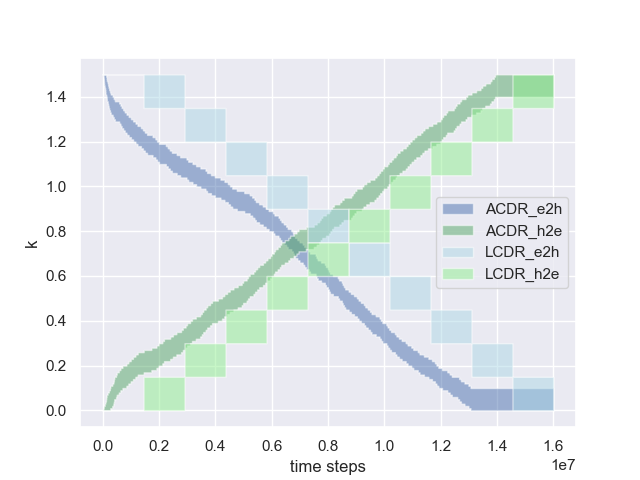
In this study, we consider two methods to update the interval . The manner in which the interval is updated during curriculum learning is illustrated in Fig. 2. In the first method, the upper and lower bounds of the interval gradually decrease as
| (9) |
given the initial interval . In all experiments, we set . This decrease rule represents an easy2hard curriculum because smaller values of and correspond to a higher walking difficult. For example, when , the leg does not move. The second method pertains to a hard2easy curriculum, i.e.,
| (10) |
We set the initial interval as . In this state, the robot cannot move the broken leg, and its ability to address this failure is gradually enhanced. Notably, although the easy2hard curriculum is commonly used in curriculum learning, the hard2easy curriculum is more effective than the easy2hard configuration in accomplishing the task. The difference between the two frameworks is discussed in Section IV-D.
III-D Reward function
In the analysis, we introduce a slightly modified reward function instead of using the commonly applied function described in [24], because the existing reward function [24] is likely to result in a conservative policy in which the robot does not walk but remains in place. The existing reward function [24] can be defined by
| (11) |
where is the walking speed, is the vector of joint torques, and is the contact force. The reward function in Eq. (11) yields a reward of even when the robot falls or remains stationary without walking. Therefore, this reward function is likely to lead to a conservative policy. To ensure active walking of the robot, we modify the reward function as
| (12) |
where
| (13) |
Preliminary experiments demonstrate that the modified reward function in Eq. (12) can ensure more active walking of the robots.
IV Experiments
We conduct experiments in the Ant-v2 environment provided by OpenAI Gym [25]. This environment runs on the simulation software MuJoCo [26], and the task is aimed at realizing rapid advancement of the quadruped robot, as shown in Fig. 1. To realize reinforcement learning, we use the PPO algorithm [23], which is suitable for high-dimensional continuous action environments.
IV-A Experiment setup
For reinforcement learning, we employ the actor and critic network consisting of two hidden layers of and neurons with activation. All networks use the Adam optimizer [27]. The related hyperparameters are listed in Table I.
| Parameter | Value |
|---|---|
| Learning rate | |
| Horizon | |
| Minibatch size | |
| epochs | |
| Clipping parameter | |
| Discount | |
| GAE parameter | |
| VF coefficient | |
| Entropy coefficient |
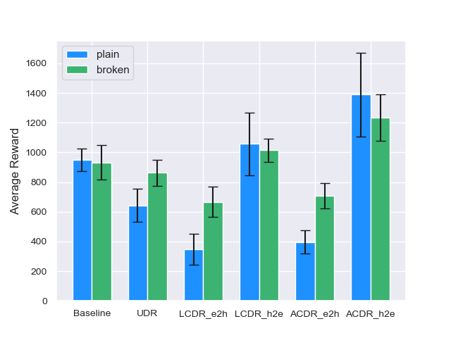
The ACDR algorithm is compared to the following three algorithms. Baseline: The baseline is a basic reinforcement learning algorithm for normal robots that implements neither dynamics randomization nor curriculum learning. Uniform Dynamics Randomization (UDR): UDR is a dynamics randomization algorithm that is based on the uniform distribution and does not implement curriculum learning. Linear Curriculum Dynamics Randomization (LCDR): In the LCDR algorithm, the interval is linearly updated. Detail of the LCDR can be found in A. Similar to the ACDR, the LCDR uses the easy2hard and hard2easy curricula. The progress of the two curricula, the legends of which are ”LCDR_e2h” and ”LCDR_h2e”, is shown in Fig. 2.
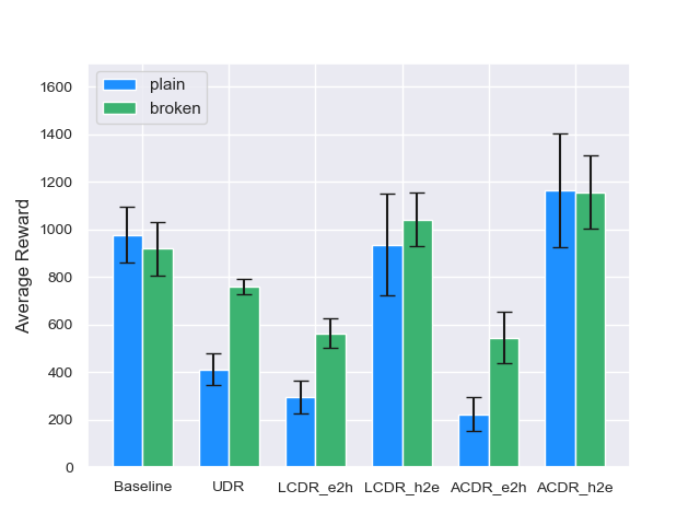
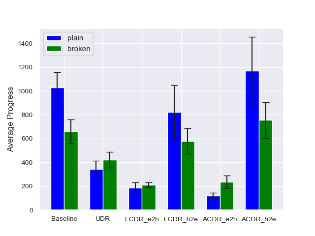
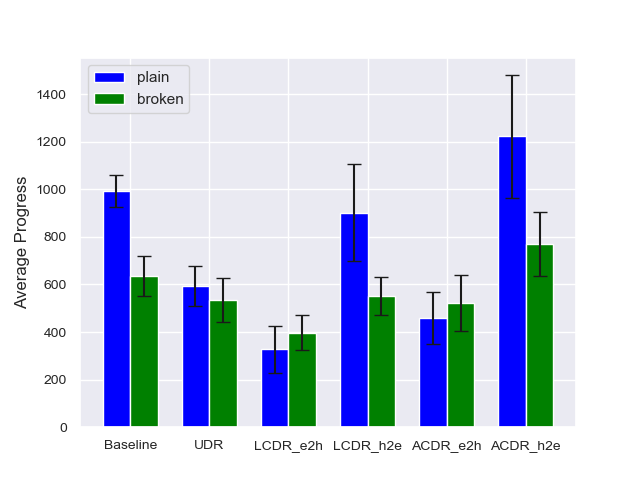
We evaluate the algorithms in terms of the average reward and average walking distance in two conditions: plain and broken. In the plain, the robots function normally, i.e., the failure coefficient is fixed at . In the broken, the robots are damaged, and randomly takes a value in . We implement each algorithm on the two conditions, with five random seeds for each framework. The average reward and average walking distance are calculated as the average of 100 trials for each seed. The average walking distance is one that is suitable for evaluating the walking ability of the robot.
IV-B Comparative evaluation with conventional algorithms
The average reward and average walking distance for all algorithms are shown in Fig. 3 and Fig. 4, respectively. In both the plain and broken conditions, UDR is inferior to the Baseline, which does not consider robot failures. This result indicates that the simple UDR cannot adapt to robot failures. The hard2easy curriculum of LCDR, denoted by LCDR_h2e, outperforms the Baseline in terms of the average reward, as shown in Fig. 3. However, LCDR_h2e corresponds to an inferior walking ability compared to that of the Baseline for both plain and broken conditions, as shown in Fig. 4. This result indicates that LCDR_h2e implements a conservative policy that does not promote walking as active as that generated by the Baseline. For both LCDR and ACDR, the hard2easy curriculum outperforms the easy2hard curriculum, as discussed in Section IV-D. Moreover, ACDR_h2e achieves the highest performance in all cases. This finding indicates that ACDR_h2e can avoid the formulation of a conservative policy by providing tasks with difficulty levels that match the progress of the robot.
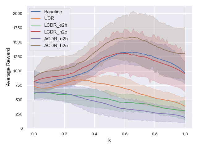
Figure 5 shows the average reward for each failure coefficient in the interval . ACDR_h2e earns the highest average reward for any , and ACDR_h2e achieves the highest performance in any failure state. Moreover, the performance of UDR, LCDR_e2h, and ACDR_e2h, deteriorate as increases. This result indicates that the robots implementing these strategies cannot learn to walk. Therefore, even when increases and it is easy to move the leg, the robots fall and do not earn rewards.
IV-C Comparative evaluation with non-curriculum learning
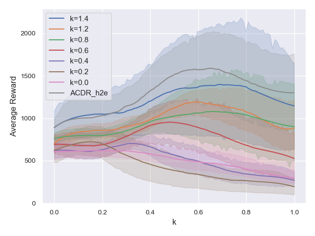
The experiment results show that the hard2easy curriculum is effective against robot failures. To evaluate whether the hard2easy curriculum contributes to an enhanced performance, we compare this framework with a non-curriculum algorithm in which the robot is trained with a fixed failure coefficient . The values of are varied as . For each , Fig. 6 shows the average reward earned by the robot on interval of the failure coefficient. ACDR_h2e still achieves the highest performance over the interval . Therefore, the hard2easy curriculum can enhance the robustness against robot failures.
IV-D Comparative evaluation between easy2hard and hard2easy curricula
The hard2easy curriculum gradually decreases the degree of robot failure and makes it easier for the robot to walk. In contrast, the easy2hard curriculum gradually increases the degree of difficulty, and eventually, the leg stops moving. Figures 3 and 4 show that the hard2easy curriculum is more effective than the easy2hard curriculum. We discuss the reason below.
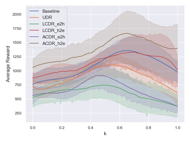
Figure 6 shows that the average reward tends to increase as increases and deteriorates as decreases. For example, corresponds to the highest average reward over the interval , whereas or yield low rewards. This result suggests that it is preferable to avoid training at to allow the robot to walk even under failure. Hence, we can hypothesize that the easy2hard curriculum, in which training is performed at at the end of training, deteriorates the robot’s ability to walk. To verify this hypothesis, we perform the same comparison as described in Section IV-B for robots trained on the interval ; in particular, in this framework, the robots are not trained at . Figures 7 and 8 show the average reward and average walking distance, respectively, and Fig. 9 shows the average reward for each over the interval . Comparison of these results with those presented in Figs. 3, 4, and 5, demonstrates that by avoiding training in the proximity of , the average rewards of LCDR_e2h and ACDR_e2h are increased. In summary, the easy2hard curriculum deteriorates the learned policy owing to the strong degree of robot failure introduced at the end of training, whereas the hard2easy curriculum does not.
Furthermore, the average rewards of UDR, LCDR_h2e, and ACDR_h2e increase, as shown in Figs. 7, 8, and 9. These results indicate that training in the proximity of is not necessary to achieve fault-tolerant robot control. Thus, interestingly, the robot can walk even when one of the legs cannot be effectively moved, without being trained under the condition.
V Conclusion
This study was aimed at realizing fault-tolerant control of quadruped robots against actuator failures. To solve the problem, we propose a reinforcement learning algorithm with adaptive curriculum dynamics randomization, abbreviated as ACDR. We apply domain randomization to fault-tolerant robot control toward Sim2Real in robotics. Furthermore, we developed an adaptive curriculum learning framework to enhance the effectiveness of domain randomization. The ACDR algorithm could formulate a single robust policy to realize fault-tolerant robot control. Notably, the ACDR algorithm can facilitate the development of a robot system that does not require any self-diagnostic modules for detecting actuator failures.
Experiment results demonstrate that the combination of curriculum learning and dynamics randomization is more effective than non-curriculum learning or non-randomization of dynamics. In addition, the hard2easy curriculum is noted to be more effective than the easy2hard curriculum. This finding suggests that it is preferable to train quadruped robots in the order of difficulty opposite to that implemented in standard curriculum learning. In future work, there are several possible research directions of improving the ACDR algorithm. A combination of automatic curriculum design (e.g. [28]) and domain randomization can be a promising direction.
Acknowledgment
This work was supported by JSPS KAKENHI Grant Number JP19K12039.
References
- [1] Volodymyr Mnih, Koray Kavukcuoglu, David Silver, Andrei A Rusu, Joel Veness, Marc G Bellemare, Alex Graves, Martin Riedmiller, Andreas K Fidjeland, Georg Ostrovski, et al. Human-level control through deep reinforcement learning. nature, 518(7540):529–533, 2015.
- [2] John Schulman, Sergey Levine, Pieter Abbeel, Michael Jordan, and Philipp Moritz. Trust region policy optimization. In International conference on machine learning, pages 1889–1897. PMLR, 2015.
- [3] Sergey Levine, Chelsea Finn, Trevor Darrell, and Pieter Abbeel. End-to-end training of deep visuomotor policies. The Journal of Machine Learning Research, 17(1):1334–1373, 2016.
- [4] Josh Tobin, Rachel Fong, Alex Ray, Jonas Schneider, Wojciech Zaremba, and Pieter Abbeel. Domain randomization for transferring deep neural networks from simulation to the real world. In 2017 IEEE/RSJ International Conference on Intelligent Robots and Systems (IROS), pages 23–30. IEEE, 2017.
- [5] Xue Bin Peng, Marcin Andrychowicz, Wojciech Zaremba, and Pieter Abbeel. Sim-to-real transfer of robotic control with dynamics randomization. In 2018 IEEE international conference on robotics and automation (ICRA), pages 1–8. IEEE, 2018.
- [6] Jie Tan, Tingnan Zhang, Erwin Coumans, Atil Iscen, Yunfei Bai, Danijar Hafner, Steven Bohez, and Vincent Vanhoucke. Sim-to-real: Learning agile locomotion for quadruped robots. arXiv preprint arXiv:1804.10332, 2018.
- [7] Ivana Kruijff-Korbayová, Francis Colas, Mario Gianni, Fiora Pirri, Joachim de Greeff, Koen Hindriks, Mark Neerincx, Petter Ögren, Tomáš Svoboda, and Rainer Worst. Tradr project: Long-term human-robot teaming for robot assisted disaster response. KI-Künstliche Intelligenz, 29(2):193–201, 2015.
- [8] Fan Yang, Chao Yang, Di Guo, Huaping Liu, and Fuchun Sun. Fault-aware robust control via adversarial reinforcement learning. arXiv preprint arXiv:2011.08728, 2020.
- [9] Ayaka Kume, Eiichi Matsumoto, Kuniyuki Takahashi, Wilson Ko, and Jethro Tan. Map-based multi-policy reinforcement learning: enhancing adaptability of robots by deep reinforcement learning. arXiv preprint arXiv:1710.06117, 2017.
- [10] Muhamad Azhar, A Alobaidy, Jassim Abdul-Jabbar, and Saad Saeed. Faults diagnosis in robot systems: A review. Al-Rafidain Engineering Journal (AREJ), 25:164–175, 12 2020.
- [11] Nicolas Heess, Dhruva TB, Srinivasan Sriram, Jay Lemmon, Josh Merel, Greg Wayne, Yuval Tassa, Tom Erez, Ziyu Wang, SM Eslami, et al. Emergence of locomotion behaviours in rich environments. arXiv preprint arXiv:1707.02286, 2017.
- [12] Wataru Okamoto and Kazuhiko Kawamoto. Reinforcement learning with randomized physical parameters for fault-tolerant robots. In 2020 Joint 11th International Conference on Soft Computing and Intelligent Systems and 21st International Symposium on Advanced Intelligent Systems (SCIS-ISIS), pages 1–4, 2020.
- [13] Bhairav Mehta, Manfred Diaz, Florian Golemo, Christopher J Pal, and Liam Paull. Active domain randomization. In Conference on Robot Learning, pages 1162–1176. PMLR, 2020.
- [14] Farzad Abdolhosseini. Learning locomotion: symmetry and torque limit considerations. PhD thesis, University of British Columbia, 2019.
- [15] Yoshua Bengio, Jérôme Louradour, Ronan Collobert, and Jason Weston. Curriculum learning. In Proceedings of the 26th annual international conference on machine learning, pages 41–48, 2009.
- [16] Diego Rodriguez and Sven Behnke. Deepwalk: Omnidirectional bipedal gait by deep reinforcement learning. In 2021 IEEE International Conference on Robotics and Automation (ICRA), pages 3033–3039, 2021.
- [17] Ozsel Kilinc and G. Montana. Follow the object: Curriculum learning for manipulation tasks with imagined goals. ArXiv, abs/2008.02066, 2020.
- [18] Sha Luo, Hamidreza Kasaei, and Lambert Schomaker. Accelerating reinforcement learning for reaching using continuous curriculum learning. In 2020 International Joint Conference on Neural Networks (IJCNN), pages 1–8. IEEE, 2020.
- [19] Rui Wang, Joel Lehman, Jeff Clune, and Kenneth O. Stanley. Paired open-ended trailblazer (POET): endlessly generating increasingly complex and diverse learning environments and their solutions. CoRR, abs/1901.01753, 2019.
- [20] Zhaoming Xie, Hung Yu Ling, Nam Hee Kim, and Michiel van de Panne. Allsteps: Curriculum-driven learning of stepping stone skills. In Proc. ACM SIGGRAPH / Eurographics Symposium on Computer Animation, 2020.
- [21] Daniele Reda, Tianxin Tao, and Michiel van de Panne. Learning to locomote: Understanding how environment design matters for deep reinforcement learning. CoRR, abs/2010.04304, 2020.
- [22] Richard S Sutton and Andrew G Barto. Reinforcement learning: An introduction. MIT press, 2018.
- [23] John Schulman, Filip Wolski, Prafulla Dhariwal, Alec Radford, and Oleg Klimov. Proximal policy optimization algorithms. arXiv preprint arXiv:1707.06347, 2017.
- [24] John Schulman, Philipp Moritz, Sergey Levine, Michael Jordan, and Pieter Abbeel. High-dimensional continuous control using generalized advantage estimation. arXiv preprint arXiv:1506.02438, 2015.
- [25] Greg Brockman, Vicki Cheung, Ludwig Pettersson, Jonas Schneider, John Schulman, Jie Tang, and Wojciech Zaremba. Openai gym. arXiv preprint arXiv:1606.01540, 2016.
- [26] Emanuel Todorov, Tom Erez, and Yuval Tassa. Mujoco: A physics engine for model-based control. In 2012 IEEE/RSJ International Conference on Intelligent Robots and Systems, pages 5026–5033. IEEE, 2012.
- [27] Diederik P. Kingma and Jimmy Ba. Adam: A method for stochastic optimization. In Yoshua Bengio and Yann LeCun, editors, 3rd International Conference on Learning Representations, ICLR 2015, San Diego, CA, USA, May 7-9, 2015, Conference Track Proceedings, 2015.
- [28] Michael Dennis, Natasha Jaques, Eugene Vinitsky, Alexandre Bayen, Stuart Russell, Andrew Critch, and Sergey Levine. Emergent complexity and zero-shot transfer via unsupervised environment design. In H. Larochelle, M. Ranzato, R. Hadsell, M. F. Balcan, and H. Lin, editors, Advances in Neural Information Processing Systems, volume 33, pages 13049–13061. Curran Associates, Inc., 2020.
Appendix A Linear Curriculum Dynamics Randomization
The LCDR updates the interval at the discrete timestep , where is defined as
| (14) |
where is the predetermined total learning time, and is the floor function. We set in the experiments. Similar to the ACDR, the LCDR implements two curricula: easy2hard and hard2easy. Given the initial interval , the easy2hard curriculum updates the interval as
| (15) |
where the update amount is defined as
| (16) |
where is the maximum value of the failure coefficient. In addition, the hard2easy curriculum updates the interval as
| (17) |
given the initial interval