Regularizing Nighttime Weirdness: Efficient Self-supervised Monocular Depth Estimation in the Dark
Abstract
Monocular depth estimation aims at predicting depth from a single image or video. Recently, self-supervised methods draw much attention since they are free of depth annotations and achieve impressive performance on several daytime benchmarks. However, they produce weird outputs in more challenging nighttime scenarios because of low visibility and varying illuminations, which bring weak textures and break brightness-consistency assumption, respectively. To address these problems, in this paper we propose a novel framework with several improvements: (1) we introduce Priors-Based Regularization to learn distribution knowledge from unpaired depth maps and prevent model from being incorrectly trained; (2) we leverage Mapping-Consistent Image Enhancement module to enhance image visibility and contrast while maintaining brightness consistency; and (3) we present Statistics-Based Mask strategy to tune the number of removed pixels within textureless regions, using dynamic statistics. Experimental results demonstrate the effectiveness of each component. Meanwhile, our framework achieves remarkable improvements and state-of-the-art results on two nighttime datasets. Code is available at https://github.com/w2kun/RNW.
1 Introduction
Monocular depth estimation is a fundamental topic in computer vision as it has wide range of applications in augmented reality [35], robotics [11] and autonomous driving [34], etc. It often needs dense depth maps to learn the mapping from color images to the depth maps in supervised settings [12, 47, 50]. However, high-quality depth data are costly collected in a broad range of environments by using expensive depth sensors (e.g. LiDAR and TOF). Hence, many efforts have been made to develop self-supervised approaches [14, 54, 24, 52], which train a depth network to estimate depth maps by exploring geometry cues in videos, i.e., reconstructing a target view (or frame) from another view, instead of utilizing high-quality depth data. Furthermore, their performances are comparable to the supervised methods in well-lit environments, such as KITTI [13] and Cityscapes [10]. Unfortunately, there are a very few works to handle with more challenging nighttime scenarios. Thus we focus on nighttime self-supervised depth estimation.
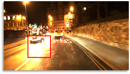
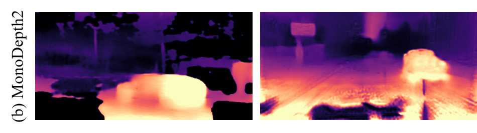
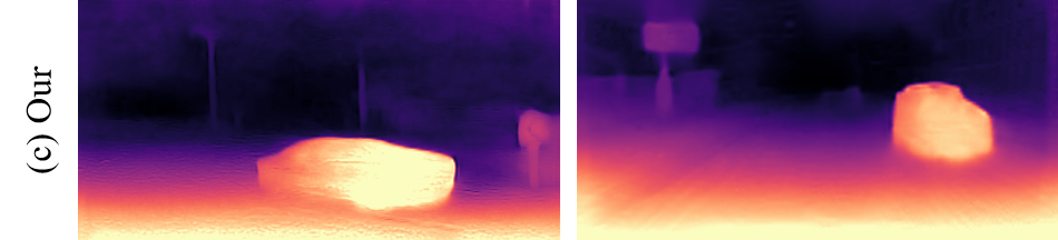
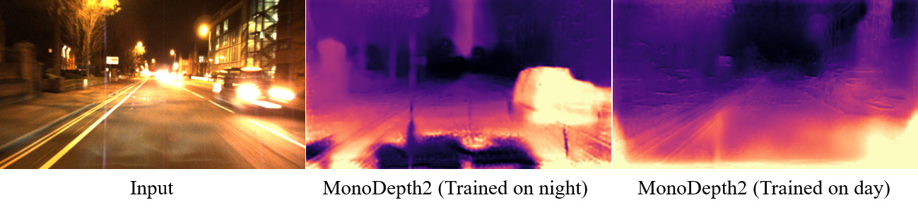
Actually, the nighttime scenario includes two important problems, low visibility and varying illuminations, resulting in that most of the existing self-supervised methods (e.g., MonoDepth2 [15]) produce a weird depth output (see Fig.1). 1) Low visibility usually creates textureless areas. For example, the cyan dashed box in the left of Fig.1 shows a dark region with indistinguishable visual texture. This textureless aggravates depth maps with big holes in the left of Fig. 1, though they may be used to correctly reconstruct the target view by sampling nearby pixels with similar brightness. 2) Varying illuminations from flickering streetlights or moving cars, undermine the brightness consistency assumption in the right of Fig.1, where the two image patches with different brightness are cropped from the same place of two temporally adjacent frames. This inconsistency brings an imperfect reconstruction of the target view, that is, a high training loss, which also produces non-smooth depth map in the right of Fig. 1. Clearly, the incorrect depth prediction (e.g., non-smoothness and big holes) indicates a failure of training the depth network.
To address these two problems, in this paper we propose an efficient nighttime self-supervised framework for depth estimation with three improvements. Firstly, we introduce Priors-Based Regularization (PBR) module to constrain the incorrect depth in neighborhoods of depth references, and prevent the depth network from being incorrectly trained. This constraint is implemented by learning prior depth distribution from unpaired references in an adversarial manner. Furthermore, 2D coordinates are encoded as an additional input of PBR to find useful depth distribution, which is related with its pixel location. Secondly, we leverage Mapping-Consistent Image Enhancement (MCIE) module to deal with the low visibility. Although image enhancement methods, e.g., Contrast Limited Histogram Equalization (CLHE) [37], can be used to achieve remarkable results on low-light images [9, 23], they are difficult to handle the correspondence among video frames, which is essential to self-supervised depth estimation. Thus, we extend the CLHE method to keep brightness consistency while enhancing low-visible video frames. Finally, we present Statistics-Based Mask (SBM) to tackle textureless regions. Though Auto-Mask [15] is a widely used strategy to efficiently choose textureless regions, its dependence on photometric loss makes it unable to adjust the numbers of removed pixels. To compensate this weakness, we introduce SBM to better handle nighttime scenarios by flexibly tuning masked pixels using dynamic statistics. In short, our contributions can be summarized as three-fold:
-
•
We propose Priors-Based Regularization module to learn distribution knowledge from unpaired references and prevent model from being incorrectly trained.
-
•
We leverage Mapping-Consistent Image Enhancement module to deal with low visibility in the dark and maintain brightness consistency.
-
•
We present Statistics-Based Mask to better handle textureless regions, by using dynamic information. Together, these contributions yield state-of-the-art performance in nighttime depth estimation task and efficiently reduce the weirdness in depth outputs.
2 Related Work
Self-supervised Depth Learning from Videos. SfMLearner [54] is a pioneering work in this task. It jointly learns to predict depth and relative pose of the camera, which is supervised by reconstruction of target frame. This process is based on the assumption of static scene while moving objects violate it. To address this problem, previous works have employed optical flow [56, 48, 38] and pre-trained segmentation models [16, 33, 7] to compensate and mask pixels within moving objects, respectively. Occlusion is also a challenge. MonoDepth2 has provided a minimum reprojection loss
to deal with it. Besides, approaches with geometry priors, such as normal [46, 29] and geometry consistency [2] have been exploited for better performance. Recently, PackNet [18] has proposed a novel network architecture to learn detail-preserving representations. FM [41] have leveraged more informative feature metric loss to address the problem of textureless regions. These methods offer ideas to improve the performance of self-supervised depth estimation in daytime environments but think little of more challenging nighttime scenarios.
Nighttime Self-supervised Learning Methods. Nighttime self-supervised depth estimation is a relatively under-explored topic as a result of its numerous challenges. Existing works have explored approaches to predict depth from thermal images [25, 30]. However, thermal images have less texture details and limited resolution. Thermal cameras are also expensive. Defeat-Net [42] has been proposed to simultaneously learn cross-domain feature representation and depth estimation to acquire a more robust supervision. Nevertheless, it is unable to tackle the low visibility and varying illuminations. ADFA [43] considers this problem as one of domain adaption and has adapted a network trained on daytime data to work for nighttime images. It aims to transfer knowledge from daytime to nighttime data.
Different from ADFA, we only use prior depth distribution from daytime data as regularization and directly exploit depth estimation knowledge from nighttime scenes.
Domain Adaptation in Depth Estimation. Domain adaptation (DA) [44], as a subproject of transfer learning [55], aims to efficiently leverage prior knowledge learned from source domain. In depth estimation, an important application is to close the gap [1, 53, 17] between synthetic [4, 3] and real-world data, for mitigating the need for large-scale real-world ground truth. For better use of geometry structure, GASDA [51] has been performed to exploit epipolar geometry of stereo images. CoMoDA [27] has been applied to continuously adapt a pre-trained model on test videos. The prior knowledge is also employed in our framework but is to regularize training.
Low-light Image Enhancement. Image enhancement is a resultful approach to improve the brightness and contrast of images. Retinex [28] decomposes an image into reflectance and illumination. Histogram equalization based methods (e.g. CLHE [37]) readjustment the brightness level of pixels. Recently, methods [9, 49] combining Retinex with Convolutional Neural Network (CNN) have shown impressive results. Previous learning-based works [6, 8] require paired data. To address this problem, efforts have been put into exploring approaches with unpaired inputs [23] or zero-reference [19]. Although these methods have proven to be effective, they pay no attention to the brightness correspondence among frames which is essential for self-supervised training of depth estimation.
3 Method
In this section, we propose a novel self-supervised framework to learn depth estimation from nighttime videos. Before presenting it, we first introduce a basic self-supervised training with necessary notations.
3.1 Self-supervised Training
In self-supervised depth estimation, the learning problem is considered as a view-synthesis process. It reconstructs target frame from the viewpoint of each source image by performing a reprojection using depth and relative pose . In the setting of monocular training, and are predicted by two neural networks via and , respectively. The camera intrinsic parameter is also required for projection operations. With the above variables, we can acquire a per-pixel correspondence between an arbitrary point in and another point in by
| (1) |
After that, can be reconstructed from with differentiable bilinear sampling [22] operation :
| (2) |
The model learning is based on the above warping process, i.e. reconstruct target frame from source view, and the objective is to reduce reconstruction error by optimizing and to produce more accurate outputs. Following [14], we apply and SSIM [45] together as photometric error to measure the difference between and ,
| (3) | |||
where is set to 0.85 in all experiments.
Moreover, this is an ill-posed problem as there are a large amount of possible incorrect depths which lead to the correct reconstruction of target frame given the relative pose . To address this depth ambiguity, we follow previous works [14] by applying edge-aware smoothness loss to enforce smoothness in depths,
| (4) |
where and are image gradient along horizontal and vertical axes, respectively.
3.2 Nighttime Depth Estimation Framework
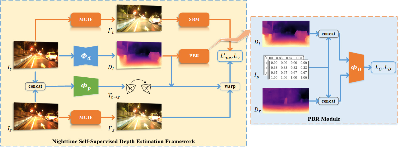
Here, we present the nighttime self-supervised depth estimation framework, which is illustrated in Fig. 2. The framework contains three improvements for nighttime environments, including PBR, MCIE and SBM, which are detailedly described next.
3.2.1 Priors-Based Regularization
Priors-Based Regularization (PBR) is to constrain the depth output in neighborhoods of depth references using adversarial manner, which is shown on the right of Fig. 2. The depth estimation network is considered as a generator and a discriminator using Patch-GAN [21] is employed in PBR. Adversarial depth maps are , where depth output is generated by , and is a referenced depth map. The discriminator is used to distinguish and , while tries to make its output indistinguishable with . In order to acquire the referenced depth maps, we train a depth estimation network to produce in a self-supervised manner using a daytime dataset. Note that, and are unpaired, thus the same scene as nighttime dataset is not required.
Besides, we find a close relationship between depth of a pixel and its position. For example, an image of driving scene usually shows a view from road to sky along vertical direction. Based on this observation, we encode the 2D coordinates of each pixel into an image as an additional input of . is composed of two single-channel maps separately indicating the coordinates along and axes and is scaled to range for normalization. Furthermore, both and are scale-ambiguity, hence it is unreasonable to unify their scales. We apply to perform normalization in depth maps to address the misalign of their scales,
| (5) |
where computes average along space dimension. Let denote the concatenation operation along channel dimension, and are network weights of and , and present a set of and , respectively, then the optimization objective for PBR can be written as
| (6) | ||||
in which the loss format in [32] is adopted for better convergence.
Remark. It is hard to instantiate the depth of a specific sample from a general depth distribution, since the depths are distributed in a range rather than a certain value. But it is easier to find a outlier (in our case weird depth value) as it greatly deviate from expected outputs. This is the reason why we use PBR as a regularizer. In addition, the application for PBR is not limited to nighttime depth estimation, but can also be extended to other similar tasks.
3.2.2 Mapping-Consistent Image Enhancement
Mapping-Consistent Image Enhancement (MCIE) is adapted from Contrast Limited Histogram Equalization[37] (CLHE) algorithm to meet the need for keeping brightness-consistency, which is essential for self-supervised depth estimation. This is implemented by using a brightness mapping function and applying it to target frame and source frames together, i.e.
| (7) |
is a single-value mapping function, which maps an input brightness to single certain output. By this way, the brightness consistency among target and source frames is naturally maintained.
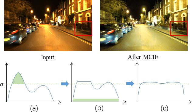
We show the primary steps to compute at the bottom of Fig. 3. Supposing the frequency distribution of input image is given, where is the frequency of brightness level . Firstly, we clip the frequency greater than the preset parameter to avoid the amplification of noise signal. Secondly, the clipped frequency is evenly filled to each brightness level, as shown in the subfigure (b). Finally, can be obtained with cumulative distribution through
| (8) |
where and separately indicate the minimum and maximum of , presents the number of brightness level (commonly 256 in color images).
MCIE brings higher visibility and more details to nighttime images. We illustrate it with the top two images in Fig. 3, where we can see a remarkable improvement on brightness and contrast, especially within the area framed by red box. MCIE only enhances image when computing photometric loss and doesn’t change the input of networks. It redefine the warping process as
| (9) |
Accordingly, the photometric loss is adapted to use enhanced images through
| (10) | |||
3.2.3 Statistics-Based Mask
We introduce Statistics-Based Mask (SBM) to compensate Auto-Mask [15] (AM) strategy as it is unable to adjust the number of removed pixels due to the dependence on photometric loss. Let denote Iverson bracket. AM produces a mask between target and source frames by
| (11) |
Unlike AM, SBM uses dynamic statistics to flexibly tune the masked pixels. During training, SBM computes the difference between target frame and each source frame by and employs Exponentially Weighted Moving Average (EWMA) to obtain the mean in recent samples, which is figured by
| (12) |
where is the current time and is momentum parameter that is set to 0.98 in our experiments. It is more stable and reflects global statistics. To tune masked pixels, a parameter indicating the percentile of requires to be defined and can be used to generate the mask between target and source frames through
| (13) |
where computes the th percentile of . We combine with via element-wise product to make the final mask used in our framework, i.e.
| (14) |
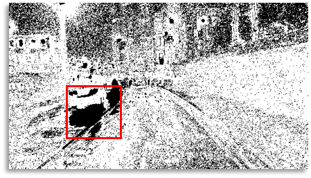
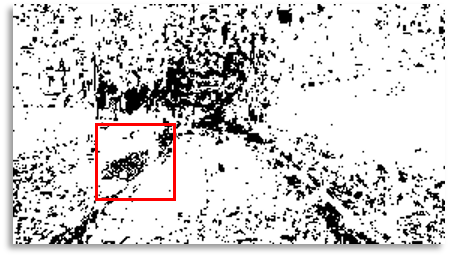
The visual comparison between and is shown in Fig. 4. It can be seen that is more effective in masking textureless regions (e.g. the sky and the bright light spot framed by red box). We employ together with , since can prevent large errors from being incorporated, which works like a regularizer.
3.2.4 Final Loss
4 Experiment
| Method | \cellcolor[RGB]244,176,132Abs Rel | \cellcolor[RGB]244,176,132Sq Rel | \cellcolor[RGB]244,176,132RMSE | \cellcolor[RGB]244,176,132RMSE log | \cellcolor[RGB]155,194,230 | \cellcolor[RGB]155,194,230 | \cellcolor[RGB]155,194,230 |
|---|---|---|---|---|---|---|---|
| \cellcolor[RGB]198,224,180RobotCar-Night | |||||||
| MonoDepth2 [15] | 0.3999 | 7.4511 | 6.6416 | 0.4429 | 0.7444 | 0.8921 | 0.9280 |
| SfMLearner [54] | 0.6754 | 15.4334 | 9.4324 | 0.6046 | 0.5465 | 0.8003 | 0.8733 |
| SC-SfMLearner [2] | 0.6029 | 16.0173 | 9.2453 | 0.5620 | 0.7185 | 0.8722 | 0.9091 |
| PackNet [18] | 0.2836 | 4.0257 | 5.3864 | 0.3351 | 0.7425 | 0.9143 | 0.9560 |
| FM [41] | 0.3953 | 7.5579 | 6.7002 | 0.4391 | 0.7605 | 0.8943 | 0.9299 |
| DeFeat-Net [42] | 0.3929 | 4.8955 | 6.3429 | 0.4236 | 0.6256 | 0.8290 | 0.8992 |
| MonoDepth2 (Day) | 0.3211 | 1.8672 | 4.9818 | 0.3568 | 0.4446 | 0.7813 | 0.9353 |
| FM (Day) | 0.2928 | 1.5380 | 4.5951 | 0.3337 | 0.4888 | 0.8054 | 0.9497 |
| Reg Only | 0.5006 | 3.7608 | 6.6351 | 0.7518 | 0.2841 | 0.5643 | 0.8156 |
| Our | 0.1205 | 0.5204 | 2.9015 | 0.1633 | 0.8794 | 0.9688 | 0.9896 |
| \cellcolor[RGB]198,224,180nuScenes-Night | |||||||
| MonoDepth2 [15] | 1.1848 | 42.3059 | 21.6129 | 1.5699 | 0.1842 | 0.3598 | 0.5044 |
| SfMLearner [54] | 0.6004 | 8.6346 | 15.4351 | 0.7522 | 0.2145 | 0.4166 | 0.5961 |
| SC-SfMLearner [2] | 1.0508 | 30.5865 | 19.6004 | 0.8854 | 0.1823 | 0.3673 | 0.5422 |
| PackNet [18] | 1.5675 | 61.5101 | 25.8318 | 1.3717 | 0.1387 | 0.2980 | 0.4313 |
| FM [41] | 1.1383 | 41.6166 | 20.8481 | 1.1483 | 0.2376 | 0.4252 | 0.5650 |
| Our | 0.3150 | 3.7926 | 9.6408 | 0.4026 | 0.5081 | 0.7776 | 0.8959 |
In this section, the proposed framework is evaluated through series experiments and is compared with state-of-the-art (SOTA) methods. Before reporting it, we firstly introduce the RobotCar-Night and nuScenes-Night datasets, on which all methods are tested, then describe the implementation details. Finally, we show the ablation study that demonstrate the effectiveness of PBR, MCIE and SBM.
4.1 Dataset
RobotCar-Night. Oxford RobotCar [31] dataset contains a large amount of data collected from one route through central Oxford, and covers various weather and traffic conditions. We build RobotCar-Night using the left images of the front stereo-camera (Bumblebee XB3) data from the sequences captured on 2014-12-16-18-44-24 and images are cropped to for excluding car-hood. The training set is formed from the first 5 splits, in which frames while camera stops moving are removed. The front LMS laser sensor data and INS data are used along with the official toolbox, to generate depth ground truth for testing. For more accurate evaluation, we manually pick up high-quality outputs. As a result, the RobotCar-Night dataset contains more than 19k training sequences and 411 test samples.
nuScenes-Night. nuScenes [5] is a large-scale dataset for autonomous driving, which is composed of 1000 diverse driving scenes in Boston and Singapore, where each scene is presented by a video of 20 second length. We firstly select 60 nighttime scenes in total. These scenes are more challenging than RobotCar, due to lower visibility and more complicated traffic conditions. Images are firstly cropped to . The front camera data from part of scenes are used to build training set and data from top LiDAR sensor in rest scenes are employed with officially released toolbox to generate depth ground truth. In summary, nuScenes-Night contains more than 10k training sequences and 500 test samples.
4.2 Implementation Detail
Our depth estimation network is based on U-Net [39] architecture, i.e. an encoder-decoder with skip connections. The encoder is a ResNet-50 [20], with fully-connected layer removed and maxpooling replaced by a stride convolution. Depth decoder contains five convolutional layers and uses nearest interpolation for up-sampling. Sigmoid and Leaky Relu nonlinearities are separately employed at the output and elsewhere. Pose prediction network is structured with ResNet-18, and outputs a vector of six element length for each sample. in PBR is a Patch-GAN [21] based discriminator with three convolutional layers of kernel size.
In experiments on RobotCar-Night, the two parameters in MCIE and SBM are set to and , respectively. In final loss, , and are set. The data captured on 2014-12-09-13-21-02 from Oxford RobotCar is employed to train the network . For nuScenes-Night, and is set to and , respectively. , and are configured for final loss. Other scenes containing daytime images in nuScenes are used to train . Notice that, the scene for training is not limited to daytime. The reasons of using daytime dataset relies on that models are more easier to trained on daytime environments. For more information about scene selection and parameter setting, please refer to supplementary material (Supp).
Our models are implemented in PyTorch[36], trained for 20 epochs on four RTX2080TI GPUs using Adam[26] optimizer, with and input resolution for RobotCar-Night and nuScenes-Night, respectively. The learning rate is initialized as , linearly warmed up to after 500 iterations and halved at 15th epochs. We apply seven standard metrics for testing, including Abs Rel, Sq Rel, RMSE, RMSE log, , and . For more information about test metrics, please see Supp. During evaluation, we restrict the maximum depth to 40m and 60m for RobotCar-Night and nuScenes-Night datasets, respectively. Moreover, the scale between predicted depth and ground truth depth is aligned using a scale factor introduced by [54]
| (16) |
The predicted depth is multiplied with before evaluation, which called median scaling.
4.3 Compare with SOTA Methods
Here, we compare our method with several SOTA approaches, including SfMLearner [54], SC-SfMLearner [2], MonoDepth2 [15], PackNet [18] and FM [41]. All methods are evaluated on both RobotCar-Night and nuScenes-Night datasets. The results are reported in Table 1 and we choose the Sq Rel metric for subsequent analysis. In general, our method significantly outperforms other competitors and shows remarkable improvements on each evaluation metric. It improves the baseline method by and on RobotCar-Night and nuScenes-Night, respectively. Compared to PackNet, which employs expensive 3D convolution to learn detail-preserving representations, our method is more lightweight and separately achieves an improvement of and on the two datasets. Also, and improvements can be seen in comparison with the recent FM method, which introduces feature-metric loss to constrain the loss landscapes to form proper convergence basins.
Furthermore, we conduct several validation experiments and report the results at the second part of RobotCar-Night. Models labeled with (Day) are trained on daytime dataset and directly tested on nighttime scenes. They score higher on the first four error metrics but worse on the last three accuracy metrics, indicating their weakness on prediction accuracy. See Supp for more analysis. Reg Only is trained with solely PBR regularization. It doesn’t work well, since just constraining the distribution consistency with referenced depth maps is not enough to infer the depth of a specific image. This is also the reason we use photometric loss as primary constraint and PBR loss as regularization in our framework.
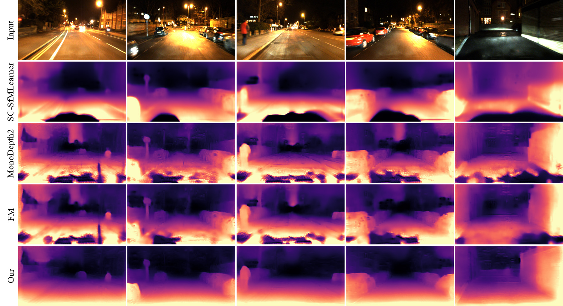
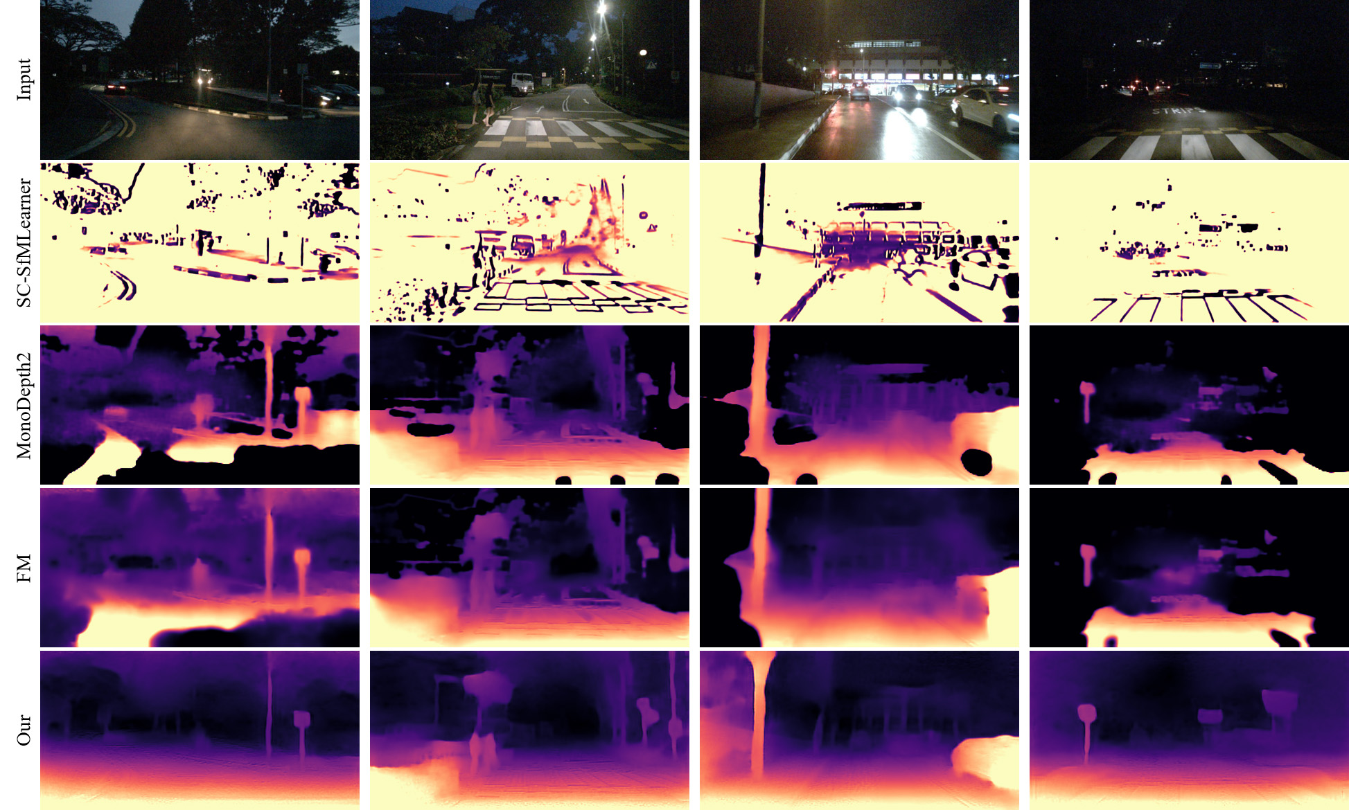
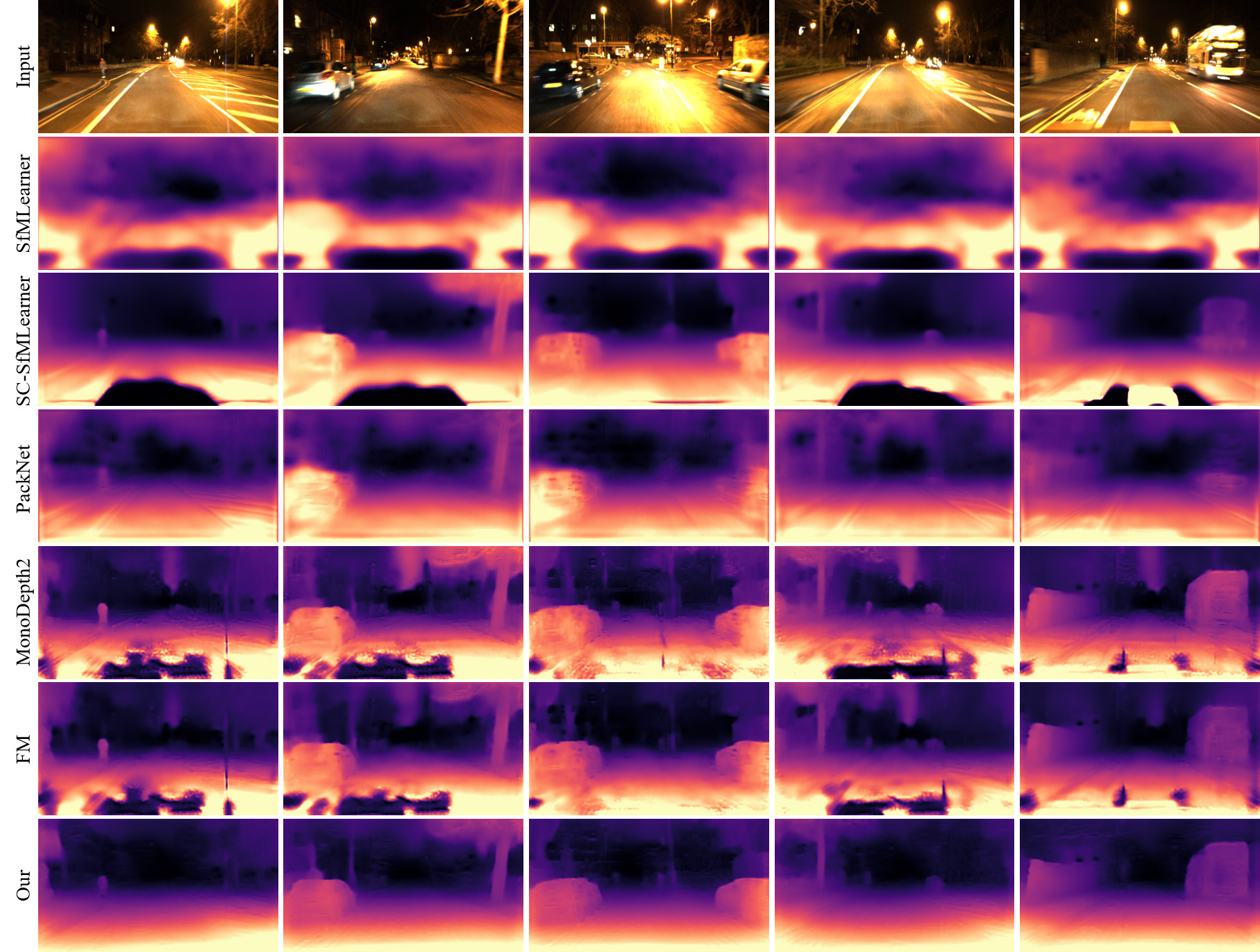
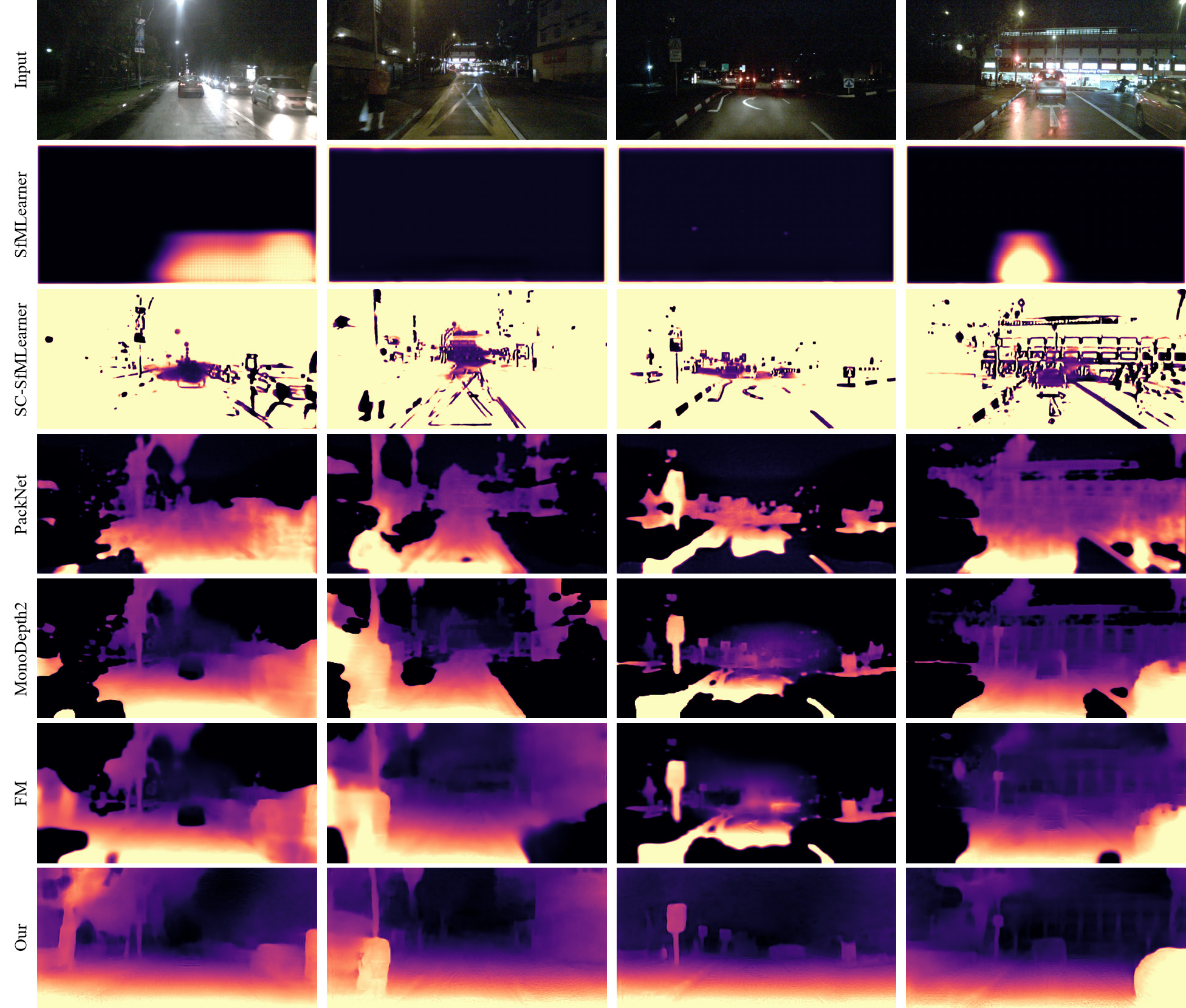
The qualitative results on RobotCar-Night and nuScenes-Night are reported in Figs. 13 and 14, respectively. We compare our method with three SOTA approaches, including SC-SfMLearner [2], MonoDepth2 [15] and FM [41]. In general, the SOTAs fail to produce smooth depth maps and miss some details of objectives. By contrast, the proposed framework greatly alleviates the non-smoothness and produces higher quality depth outputs. In Fig. 14, our model is still able to make a plausible guess on very dark scenes which are even challenging for human eye. It demonstrates the effectiveness of our method to regularize weird outputs in nighttime depth estimation.
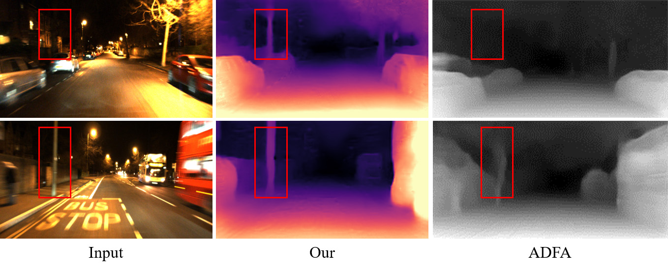
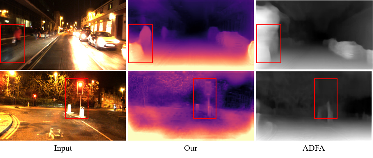
More importantly, we compare with ADFA [43] in qualitative results. It firstly focuses on nighttime depth estimation and leverages adversarial domain adaptation to address this problem. In the two samples of Fig. 6, ADFA produces blurry outputs and is unable to predict the accurate depth of the two objects framed by red boxes. In contrast, our results are clearer and more accurate. Compared to ADFA, the proposed method learns to predict depth directly from nighttime data instead of transferring knowledge learned from daytime scenarios. This enables models to better adapt to nighttime environments, thus achieves better performance.
| Method | \cellcolor[RGB]244,176,132Abs Rel | \cellcolor[RGB]244,176,132Sq Rel | \cellcolor[RGB]244,176,132RMSE | \cellcolor[RGB]244,176,132RMSE log | \cellcolor[RGB]155,194,230 | \cellcolor[RGB]155,194,230 | \cellcolor[RGB]155,194,230 |
|---|---|---|---|---|---|---|---|
| \cellcolor[RGB]198,224,180RobotCar-Night | |||||||
| MonoDepth2 | 0.400 | 7.451 | 6.642 | 0.443 | 0.744 | 0.892 | 0.928 |
| PBR Only | 0.126 | 0.539 | 2.953 | 0.168 | 0.865 | 0.970 | 0.990 |
| MCIE Only | 0.377 | 6.735 | 6.530 | 0.425 | 0.728 | 0.884 | 0.931 |
| SBM Only | 0.348 | 5.389 | 5.896 | 0.400 | 0.742 | 0.898 | 0.935 |
| PBR + MCIE | 0.122 | 0.528 | 2.914 | 0.165 | 0.875 | 0.969 | 0.989 |
| Full without | 0.128 | 0.588 | 3.112 | 0.173 | 0.856 | 0.966 | 0.989 |
| Full Method | 0.121 | 0.520 | 2.902 | 0.163 | 0.879 | 0.969 | 0.990 |
| \cellcolor[RGB]198,224,180nuScenes-Night | |||||||
| MonoDepth2 | 1.185 | 42.306 | 21.613 | 1.570 | 0.184 | 0.360 | 0.504 |
| PBR Only | 0.325 | 4.127 | 9.881 | 0.413 | 0.508 | 0.770 | 0.888 |
| MCIE Only | 1.153 | 40.741 | 21.193 | 1.511 | 0.202 | 0.377 | 0.521 |
| SBM Only | 0.779 | 25.794 | 16.657 | 0.680 | 0.354 | 0.594 | 0.744 |
| PBR + MCIE | 0.321 | 4.005 | 9.644 | 0.403 | 0.508 | 0.784 | 0.898 |
| Full without | 0.333 | 4.467 | 9.947 | 0.417 | 0.509 | 0.772 | 0.888 |
| Full Method | 0.315 | 3.793 | 9.641 | 0.403 | 0.508 | 0.778 | 0.896 |
4.4 Ablation Study
Here, we conduct a series of experiments to demonstrate the effectiveness of proposed components and report the results in Table 2. Firstly, baseline method coupled with each individual component (PBR Only, MCIE Only and SBM Only) is tested. The results in the second part show improved performance, indicating the effectiveness of each component. Among them, PBR Only performs the best. It promotes the Sq Rel by and on RC and NS, respectively. Followed by SBM Only, then MCIE Only, the former separately obtains an improvement of and while the later and on these two datasets.
Next, we further evaluate the framework by gradually enabling each component. The results are reported at PBR Only, PBR + MCIE and Full Method. In summary, the performance is improved as more components are enabled. On RC, improvements of Sq Rel are achieved by Full Method when compared to PBR Only and in comparison with PBR + MCIE. As for NS, the proportion is and , respectively.
Also, the coordinates image is tested through Full without and Full Method. Compared with the later, the Sq Rel metric of the former drops by on RC and on NS, respectively. This validates the association between image coordinates and depth distribution.
5 Conclusion
In this paper, we propose a novel framework with three improvements to effectively address the problem of self-supervised nighttime depth estimation. Priors-Based Regularization leverages prior distribution from referenced depth maps to regularize model training; Mapping-Consistent Image Enhancement module enhances image brightness and contrast while maintaining brightness consistency to deal with the low visibility in the dark; Statistics-Based Mask flexibly removes pixels within textureless regions using dynamic statistics to mitigate depth ambiguity. Benefits from these improvements, our method significantly outperforms current SOTA methods and greatly alleviate the weird outputs in nighttime depth estimation.
6 Acknowledgement
The authors would like to thank the editor and the anonymous reviewers for their critical and constructive comments and suggestions. This work was supported by the National Science Fund of China under Grant No. U1713208, 62072242 and Postdoctoral Innovative Talent Support Program of China under Grant BX20200168, 2020M681608.
References
- [1] Amir Atapour-Abarghouei and Toby P Breckon. Real-time monocular depth estimation using synthetic data with domain adaptation via image style transfer. In CVPR, pages 2800–2810, 2018.
- [2] Jiawang Bian, Zhichao Li, Naiyan Wang, Huangying Zhan, Chunhua Shen, Ming-Ming Cheng, and Ian Reid. Unsupervised scale-consistent depth and ego-motion learning from monocular video. In NIPS, volume 32, 2019.
- [3] D. J. Butler, J. Wulff, G. B. Stanley, and M. J. Black. A naturalistic open source movie for optical flow evaluation. In ECCV, pages 611–625, Oct. 2012.
- [4] Yohann Cabon, Naila Murray, and Martin Humenberger. Virtual kitti 2, 2020.
- [5] Holger Caesar, Varun Bankiti, Alex H. Lang, Sourabh Vora, Venice Erin Liong, Qiang Xu, Anush Krishnan, Yu Pan, Giancarlo Baldan, and Oscar Beijbom. nuscenes: A multimodal dataset for autonomous driving. arXiv preprint arXiv:1903.11027, 2019.
- [6] Jianrui Cai, Shuhang Gu, and Lei Zhang. Learning a deep single image contrast enhancer from multi-exposure images. TIP, 27(4):2049–2062, 2018.
- [7] Vincent Casser, Soeren Pirk, Reza Mahjourian, and Anelia Angelova. Depth prediction without the sensors: Leveraging structure for unsupervised learning from monocular videos. In AAAI, volume 33, pages 8001–8008, 2019.
- [8] Chen Chen, Qifeng Chen, Jia Xu, and Vladlen Koltun. Learning to see in the dark. In CVPR, pages 3291–3300, 2018.
- [9] Wei Chen, Wang Wenjing, Yang Wenhan, and Liu Jiaying. Deep retinex decomposition for low-light enhancement. In BMVC, 2018.
- [10] Marius Cordts, Mohamed Omran, Sebastian Ramos, Timo Rehfeld, Markus Enzweiler, Rodrigo Benenson, Uwe Franke, Stefan Roth, and Bernt Schiele. The cityscapes dataset for semantic urban scene understanding. In CVPR, pages 3213–3223, 2016.
- [11] Guilherme N DeSouza and Avinash C Kak. Vision for mobile robot navigation: A survey. TPAMI, 24(2):237–267, 2002.
- [12] Huan Fu, Mingming Gong, Chaohui Wang, Kayhan Batmanghelich, and Dacheng Tao. Deep ordinal regression network for monocular depth estimation. In CVPR, pages 2002–2011, 2018.
- [13] Andreas Geiger, Philip Lenz, Christoph Stiller, and Raquel Urtasun. Vision meets robotics: The kitti dataset. INT J ROBOT RES, 32(11):1231–1237, 2013.
- [14] Clément Godard, Oisin Mac Aodha, and Gabriel J Brostow. Unsupervised monocular depth estimation with left-right consistency. In CVPR, pages 270–279, 2017.
- [15] Clément Godard, Oisin Mac Aodha, Michael Firman, and Gabriel J Brostow. Digging into self-supervised monocular depth estimation. In ICCV, pages 3828–3838, 2019.
- [16] Ariel Gordon, Hanhan Li, Rico Jonschkowski, and Anelia Angelova. Depth from videos in the wild: Unsupervised monocular depth learning from unknown cameras. In ICCV, pages 8977–8986, 2019.
- [17] Xiao Gu, Yao Guo, Fani Deligianni, and Guang-Zhong Yang. Coupled real-synthetic domain adaptation for real-world deep depth enhancement. TIP, 29:6343–6356, 2020.
- [18] Vitor Guizilini, Rares Ambrus, Sudeep Pillai, Allan Raventos, and Adrien Gaidon. 3d packing for self-supervised monocular depth estimation. In CVPR, pages 2485–2494, 2020.
- [19] Chunle Guo, Chongyi Li, Jichang Guo, Chen Change Loy, Junhui Hou, Sam Kwong, and Runmin Cong. Zero-reference deep curve estimation for low-light image enhancement. In CVPR, pages 1780–1789, 2020.
- [20] Kaiming He, Xiangyu Zhang, Shaoqing Ren, and Jian Sun. Deep residual learning for image recognition. In CVPR, pages 770–778, 2016.
- [21] Phillip Isola, Jun-Yan Zhu, Tinghui Zhou, and Alexei A Efros. Image-to-image translation with conditional adversarial networks. In CVPR, pages 1125–1134, 2017.
- [22] Max Jaderberg, Karen Simonyan, Andrew Zisserman, and koray kavukcuoglu. Spatial transformer networks. In NIPS, volume 28, 2015.
- [23] Yifan Jiang, Xinyu Gong, Ding Liu, Yu Cheng, Chen Fang, Xiaohui Shen, Jianchao Yang, Pan Zhou, and Zhangyang Wang. Enlightengan: Deep light enhancement without paired supervision. TIP, 30:2340–2349, 2021.
- [24] Adrian Johnston and Gustavo Carneiro. Self-supervised monocular trained depth estimation using self-attention and discrete disparity volume. In CVPR, pages 4756–4765, 2020.
- [25] Namil Kim, Yukyung Choi, Soonmin Hwang, and In So Kweon. Multispectral transfer network: Unsupervised depth estimation for all-day vision. In AAAI, volume 32, 2018.
- [26] Diederik P Kingma and Jimmy Ba. Adam: A method for stochastic optimization. arXiv preprint arXiv:1412.6980, 2014.
- [27] Yevhen Kuznietsov, Marc Proesmans, and Luc Van Gool. Comoda: Continuous monocular depth adaptation using past experiences. In WACV, pages 2907–2917, 2021.
- [28] Edwin H Land. An alternative technique for the computation of the designator in the retinex theory of color vision. PNAS, 83(10):3078–3080, 1986.
- [29] Xiaoxiao Long, Lingjie Liu, Christian Theobalt, and Wenping Wang. Occlusion-aware depth estimation with adaptive normal constraints. In ECCV, pages 640–657. Springer, 2020.
- [30] Yawen Lu and Guoyu Lu. An alternative of lidar in nighttime: Unsupervised depth estimation based on single thermal image. In WACV, pages 3833–3843, 2021.
- [31] Will Maddern, Geoff Pascoe, Chris Linegar, and Paul Newman. 1 Year, 1000km: The Oxford RobotCar Dataset. IJRR, 36(1):3–15, 2017.
- [32] Xudong Mao, Qing Li, Haoran Xie, Raymond YK Lau, Zhen Wang, and Stephen Paul Smolley. Least squares generative adversarial networks. In ICCV, pages 2794–2802, 2017.
- [33] Yue Meng, Yongxi Lu, Aman Raj, Samuel Sunarjo, Rui Guo, Tara Javidi, Gaurav Bansal, and Dinesh Bharadia. Signet: Semantic instance aided unsupervised 3d geometry perception. In CVPR, pages 9810–9820, 2019.
- [34] Moritz Menze and Andreas Geiger. Object scene flow for autonomous vehicles. In CVPR, pages 3061–3070, 2015.
- [35] Richard A Newcombe, Steven J Lovegrove, and Andrew J Davison. Dtam: Dense tracking and mapping in real-time. In ICCV, pages 2320–2327. IEEE, 2011.
- [36] Adam Paszke, Sam Gross, Soumith Chintala, Gregory Chanan, Edward Yang, Zachary DeVito, Zeming Lin, Alban Desmaison, Luca Antiga, and Adam Lerer. Automatic differentiation in pytorch. 2017.
- [37] Stephen M Pizer, E Philip Amburn, John D Austin, Robert Cromartie, Ari Geselowitz, Trey Greer, Bart ter Haar Romeny, John B Zimmerman, and Karel Zuiderveld. Adaptive histogram equalization and its variations. Computer vision, graphics, and image processing, 39(3):355–368, 1987.
- [38] Anurag Ranjan, Varun Jampani, Lukas Balles, Kihwan Kim, Deqing Sun, Jonas Wulff, and Michael J Black. Competitive collaboration: Joint unsupervised learning of depth, camera motion, optical flow and motion segmentation. In CVPR, pages 12240–12249, 2019.
- [39] Olaf Ronneberger, Philipp Fischer, and Thomas Brox. U-net: Convolutional networks for biomedical image segmentation. In MICCAI, pages 234–241. Springer, 2015.
- [40] Torsten Sattler, Will Maddern, Carl Toft, Akihiko Torii, Lars Hammarstrand, Erik Stenborg, Daniel Safari, Masatoshi Okutomi, Marc Pollefeys, Josef Sivic, et al. Benchmarking 6dof outdoor visual localization in changing conditions. In CVPR, pages 8601–8610, 2018.
- [41] Chang Shu, Kun Yu, Zhixiang Duan, and Kuiyuan Yang. Feature-metric loss for self-supervised learning of depth and egomotion. In ECCV, pages 572–588. Springer, 2020.
- [42] Jaime Spencer, Richard Bowden, and Simon Hadfield. Defeat-net: General monocular depth via simultaneous unsupervised representation learning. In CVPR, pages 14402–14413, 2020.
- [43] Madhu Vankadari, Sourav Garg, Anima Majumder, Swagat Kumar, and Ardhendu Behera. Unsupervised monocular depth estimation for night-time images using adversarial domain feature adaptation. In ECCV, pages 443–459. Springer, 2020.
- [44] Mei Wang and Weihong Deng. Deep visual domain adaptation: A survey. Neurocomputing, 312:135–153, 2018.
- [45] Zhou Wang, Alan C Bovik, Hamid R Sheikh, and Eero P Simoncelli. Image quality assessment: from error visibility to structural similarity. TIP, 13(4):600–612, 2004.
- [46] Zhenheng Yang, Peng Wang, Wei Xu, Liang Zhao, and Ramakant Nevatia. Unsupervised learning of geometry with edge-aware depth-normal consistency. In AAAI, 2018.
- [47] Wei Yin, Yifan Liu, Chunhua Shen, and Youliang Yan. Enforcing geometric constraints of virtual normal for depth prediction. In ICCV, pages 5684–5693, 2019.
- [48] Zhichao Yin and Jianping Shi. Geonet: Unsupervised learning of dense depth, optical flow and camera pose. In CVPR, pages 1983–1992, 2018.
- [49] Yonghua Zhang, Jiawan Zhang, and Xiaojie Guo. Kindling the darkness: A practical low-light image enhancer. In ACM MM, pages 1632–1640, 2019.
- [50] Zhenyu Zhang, Zhen Cui, Chunyan Xu, Yan Yan, Nicu Sebe, and Jian Yang. Pattern-affinitive propagation across depth, surface normal and semantic segmentation. In CVPR, pages 4106–4115, 2019.
- [51] Shanshan Zhao, Huan Fu, Mingming Gong, and Dacheng Tao. Geometry-aware symmetric domain adaptation for monocular depth estimation. In CVPR, pages 9788–9798, 2019.
- [52] Wang Zhao, Shaohui Liu, Yezhi Shu, and Yong-Jin Liu. Towards better generalization: Joint depth-pose learning without posenet. In CVPR, pages 9151–9161, 2020.
- [53] Chuanxia Zheng, Tat-Jen Cham, and Jianfei Cai. T2net: Synthetic-to-realistic translation for solving single-image depth estimation tasks. In ECCV, pages 767–783, 2018.
- [54] Tinghui Zhou, Matthew Brown, Noah Snavely, and David G Lowe. Unsupervised learning of depth and ego-motion from video. In CVPR, pages 1851–1858, 2017.
- [55] Fuzhen Zhuang, Zhiyuan Qi, Keyu Duan, Dongbo Xi, Yongchun Zhu, Hengshu Zhu, Hui Xiong, and Qing He. A comprehensive survey on transfer learning. Proc. IEEE, 109(1):43–76, 2020.
- [56] Yuliang Zou, Zelun Luo, and Jia-Bin Huang. Df-net: Unsupervised joint learning of depth and flow using cross-task consistency. In ECCV, pages 36–53, 2018.
Appendix A Dataset Construction
Dataset for self-supervised monocular depth training in nighttime is under-explored. To make up this lack, we build two nighttime datasets, named RobotCar-Night (RC-N) and nuScenes-Night (NS-N). The two datasets consist of many video clips from Oxford RobotCar [31] and nuScenes [5], along with carefully generated ground truth using the official toolbox111Oxford RobotCar: https://github.com/ori-mrg/robotcar-dataset-sdk, nuScenes: https://github.com/nutonomy/nuscenes-devkit.
In RobotCar, the number of LiDAR points in one frame is relatively small, so multiple frames are combined to generate the ground truth depth using official scripts. This process is based on Structure-from-Motion (SFM), therefore moving objects lead to wrong outputs. For example, a generated depth map is visualized in Fig. 8. It shows an obvious mistake on the moving car framed by a red box. To tackle this problem, we manually select scenes without moving object and carefully pick up many high-quality outputs among them. This approach is different from the previous work [43], in which random sampling is used to choose test samples.
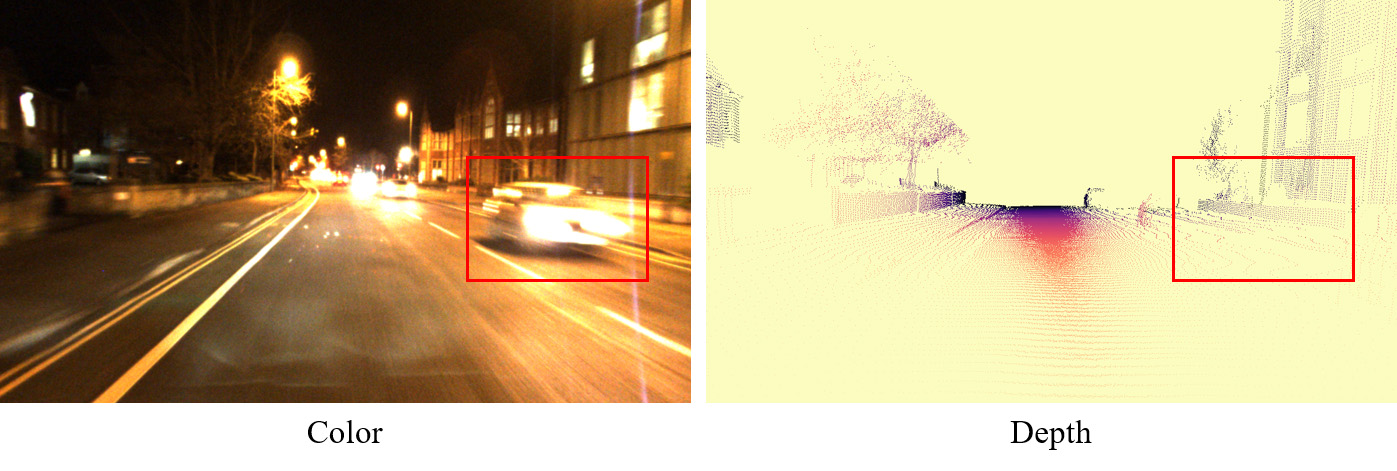
Remark. In main text, there are several samples containing moving objects in Fig. 5. These samples are from the same video sequences as RC-N but neither included in test nor training split. This is also the case for the last sample in Fig. 8.
By contrast, the LiDAR data in nuScenes contain more than 3,000 valid points in one frame and covers a wide range of depth values. Thus, data from single frame is used to prepare the ground truth depth maps and random sampling is applied to form the final test split.
Furthermore, some video clips containing daytime scenarios are selected from Oxford RobotCar and nuScenes to separately build RobotCar-Day (RC-D) and nuScenes-Day (NS-D), which are used to generate referenced depth maps.
Appendix B Parameter Setting
Here, we discuss the parameter setting about in MCIE and in SBM. Images captured in low light environments are usually noisy, thus a smaller should be set to avoid an excessive enhancement on noise. In darker scenarios, more textureless pixels need to be masked out. Therefore, should be set to a bigger value. In our experiment, is set to and on RC-N and NS-N dataset, respectively. This can be a empirical reference to set these two parameters.
To explore the effect of these two parameters, we conduct series comparison tests on RC-N and report the RMSE error in Fig. 9. The variables in the left and right chart are and , respectively. Zero indicates the corresponding module is not enabled. Overall, these two parameters impact little to the framework which performs the best when .
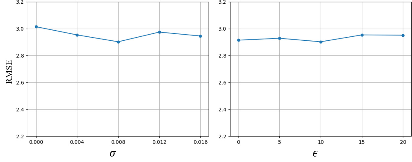
Generally speaking, and are proper ranges for and , respectively. Besides, comparison tests can help to choose the best parameter setting.
Appendix C Selection of Referenced Scene
In our framework, the reference depth maps are generated by a depth estimation network trained on RC-D and NS-D in a self-supervised manner. They provide prior knowledge about depth distributions and are unpaired with nighttime scenarios. Generally speaking, depth maps in various driving scenes can be used as references, since they share similar depth distributions. To explore the effect of different reference scenarios, we train the framework in two referenced scenarios and report quantitative results in Tab. 3. The method Our (RobotCar-Day) achieves a slightly worse but similar performance compared to Our (nuScenes-Day) and significantly outperforms other SOTA methods. This illustrates that depth maps from other scenarios are also able to regularize training.
| Method | \cellcolor[RGB]244,176,132Abs Rel | \cellcolor[RGB]244,176,132Sq Rel | \cellcolor[RGB]244,176,132RMSE | \cellcolor[RGB]244,176,132RMSE log | \cellcolor[RGB]155,194,230 | \cellcolor[RGB]155,194,230 | \cellcolor[RGB]155,194,230 |
|---|---|---|---|---|---|---|---|
| MonoDepth2 [15] | 1.1848 | 42.3059 | 21.6129 | 1.5699 | 0.1842 | 0.3598 | 0.5044 |
| SfMLearner [54] | 0.6004 | 8.6346 | 15.4351 | 0.7522 | 0.2145 | 0.4166 | 0.5961 |
| SC-SfMLearner [2] | 1.0508 | 30.5865 | 19.6004 | 0.8854 | 0.1823 | 0.3673 | 0.5422 |
| PackNet [18] | 1.5675 | 61.5101 | 25.8318 | 1.3717 | 0.1387 | 0.2980 | 0.4313 |
| FM [41] | 1.1383 | 41.6166 | 20.8481 | 1.1483 | 0.2376 | 0.4252 | 0.5650 |
| Our (nuScenes-Day) | 0.3150 | 3.7926 | 9.6408 | 0.4026 | 0.5081 | 0.7776 | 0.8959 |
| Our (RobotCar-Day) | 0.3285 | 4.3069 | 10.2651 | 0.4197 | 0.5142 | 0.7642 | 0.8813 |
Appendix D Comparison with ADFA in Challenging Cases
ADFA [43] claims three challenging cases that lead to its failure, including nighttime images with very low-illumination conditions, blurred image regions and saturated regions (bright light spots). Here, we further compare our method with ADFA in these three cases.
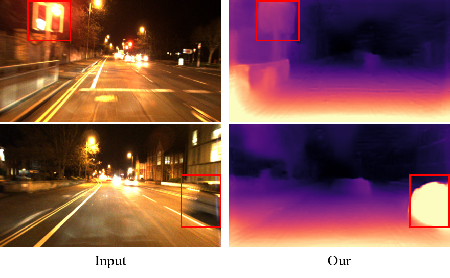
Blurred and Saturated Image Regions. Fig. 10 shows a comparison on two image samples containing saturated and blurred regions. Compared with ADFA, our method achieves better performance on presenting the shape of objects. Furthermore, two similar samples are shown in Fig. 11 to further illustrate the advantages of our method.
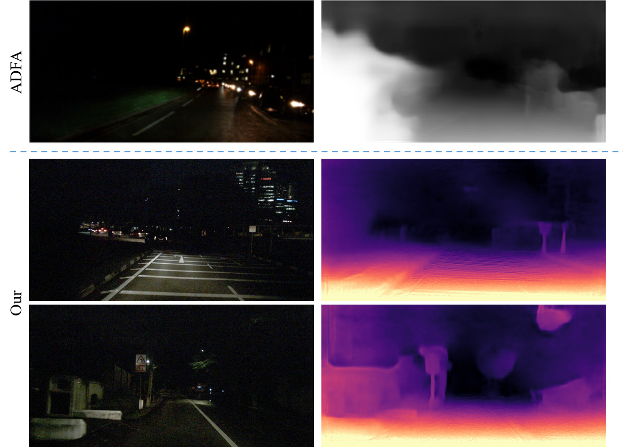
Images with very Low-Illumination Conditions. Very low-light images are a huge challenge for self-supervised depth estimation. Fig. 12 shows three samples in very low illuminated environments, where the top one and last two are generated by ADFA and our method, respectively. On the first sample, ADFA produces a blurry and inaccurate depth map. In contrast, our method is still able to make a plausible prediction on the second sample. The last sample is captured in a very dark environment. Our method makes a coarse estimation on some objectives but fails to depict the depth of entire scene.
Appendix E More Qualitative Result
Here, we show more qualitative results on RobotCar-Night and nuScenes-Night datasets in Fig. 13 and Fig. 14, respectively. Five SOTA methods are evaluated for comparison, including SfMLearner [54], SC-SfMLearner [2], PackNet [18], MonoDepth2 [15] and FM [41].
Appendix F Evaluation Metrics
There are seven standard metrics are used for evaluation, including Abs Rel, Sq Rel, RMSE, RMSE log, , and , which are presented by
| (17) |
where and separately denotes predicted and ground truth depth maps, indicates a set of valid ground truth depth values in one image, returns the number of elements in the input set.
Appendix G More discussion on experiment results
More Analysis on Experiments. In Table. 1 of main text, we show the evaluation results on RC-N. One may notice that, MonoDepth2 (Day) and FM (Day) achieve better results on the first four error metrics yet worse on the last three accuracy ones than their counterparts. Here, we present a possible explanation on this phenomenon. Fig. 15 shows two depth maps generated by MonoDepth2 (abbr. MD2) and MonoDepth2 (Day), respectively. The former produces more detailed results but with big holes while the later generates blurry outputs without holes. The big holes indicate a very large depth value and differ greatly from the Ground Truth, thus MD2 gets higher average errors on Abs_Rel, Sq_Rel, RMSE and RMSE_log. Conversely, denote the percentage of pixels below a certain threshold, therefore MD2 outperforms MD2 (Day) by more accurate predictions within non-hole areas.
Mixed Data Training. We train MD2 and FM with mixed daytime and nighttime data from nuScenes and report the results (MonoDepth2 (Mix) and FM (Mix)) in Table. 4. These two methods achieve better performance than their baselines but still keep a large gap to Our.
| Method | \cellcolor[RGB]251,229,214Abs Rel | \cellcolor[RGB]251,229,214Sq Rel | \cellcolor[RGB]251,229,214RMSE | \cellcolor[RGB]251,229,214RMSE log | \cellcolor[RGB]222,235,247 | \cellcolor[RGB]222,235,247 | \cellcolor[RGB]222,235,247 |
|---|---|---|---|---|---|---|---|
| MonoDepth2 | 1.185 | 42.306 | 21.613 | 1.570 | 0.184 | 0.360 | 0.504 |
| FM | 1.138 | 41.617 | 20.848 | 1.148 | 0.238 | 0.425 | 0.5650 |
| MonoDepth2 (Mix) | 1.070 | 38.336 | 20.117 | 1.191 | 0.269 | 0.451 | 0.586 |
| FM (Mix) | 0.956 | 34.052 | 18.794 | 0.798 | 0.305 | 0.507 | 0.652 |
| Our | 0.315 | 3.793 | 9.641 | 0.403 | 0.508 | 0.778 | 0.896 |