Regularized Optimal Transport Layers for Generalized Global Pooling Operations
Abstract
Global pooling is one of the most significant operations in many machine learning models and tasks, which works for information fusion and structured data (like sets and graphs) representation. However, without solid mathematical fundamentals, its practical implementations often depend on empirical mechanisms and thus lead to sub-optimal, even unsatisfactory performance. In this work, we develop a novel and generalized global pooling framework through the lens of optimal transport. The proposed framework is interpretable from the perspective of expectation-maximization. Essentially, it aims at learning an optimal transport across sample indices and feature dimensions, making the corresponding pooling operation maximize the conditional expectation of input data. We demonstrate that most existing pooling methods are equivalent to solving a regularized optimal transport (ROT) problem with different specializations, and more sophisticated pooling operations can be implemented by hierarchically solving multiple ROT problems. Making the parameters of the ROT problem learnable, we develop a family of regularized optimal transport pooling (ROTP) layers. We implement the ROTP layers as a new kind of deep implicit layer. Their model architectures correspond to different optimization algorithms. We test our ROTP layers in several representative set-level machine learning scenarios, including multi-instance learning (MIL), graph classification, graph set representation, and image classification. Experimental results show that applying our ROTP layers can reduce the difficulty of the design and selection of global pooling — our ROTP layers may either imitate some existing global pooling methods or lead to some new pooling layers fitting data better. The code is available at https://github.com/SDS-Lab/ROT-Pooling.
Index Terms:
Global pooling, regularized optimal transport, Bregman ADMM, Sinkhorn scaling, set representation, graph embedding.1 Introduction
As a fundamental operation of information fusion and structured data representation, global pooling achieves a global representation for a set of inputs. It makes the representation invariant to the permutation of the inputs. This operation has been widely used in many set-level machine learning tasks. In multi-instance learning (MIL) tasks [1, 2], we often leverage a global pooling operation to aggregate multiple instances into a bag-level representation. In graph representation tasks, after passing a graph through a graph neural network, we often apply a global pooling operation (or called “readout”) to merge its node embeddings into a global graph embedding [3, 4]. Besides these two representative cases, pooling layers are also necessary for convolutional neural networks (CNN) when extracting visual features [5, 6]. For the data with multi-scale clustering structures [7, 8], we can stack multiple pooling layers and derive a hierarchical pooling operation accordingly.

Currently, many different kinds of global pooling operations have been proposed. Simple operations, like add-pooling, mean-pooling (or called average-pooling), and max-pooling [9], are commonly used because of their computational efficiency. The mixture [10] and the concatenation [11, 12] of these simple pooling operations are also considered to improve their performance. More recently, some pooling methods, e.g., Network-in-Network (NIN) [13], Set2Set [14], DeepSet [15], dynamic pooling [1], and attention-based pooling layers [2, 16], are developed with learnable parameters and more sophisticated mechanisms. Although the above global pooling methods have been widely used in many machine learning models and tasks, their theoretical study is far lagged-behind. In particular, the principles of these methods are not well-interpreted in Statistics, whose rationality and effectiveness are not supported in theory. Additionally, facing so many different pooling methods, the differences and the connections among them are not thoroughly investigated. Without insightful theoretical guidance, the pooling methods’ design and selection are empirical or depend on time-consuming enumerating, which often leads to poorly-generalizable models and sub-optimal performance in practice.
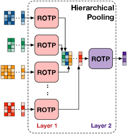
To simplify the design of global pooling in an interpretable way and boost its performance in practice, in this study, we propose a novel and solid algorithmic pooling framework to unify and generalize most existing global pooling operations through the lens of optimal transport. As illustrated in Fig. 1(a), given a batch of data, the proposed pooling operation first optimizes the joint distribution of sample indices and feature dimensions and then weights and averages the representative “sample-feature” pairs. The optimization problem in the above pooling process corresponds to a regularized optimal transport (ROT) problem. In the problem, the target joint distribution corresponds to an optimal transport (OT) plan derived under three regularizations: the smoothness of the OT plan, the uncertainty of the OT plan’s marginal distributions, and optionally the Gromov-Wasserstein (GW) discrepancy [17] between the feature-level and sample-level similarity matrices. The above pooling operation provides a generalized pooling framework with theoretical guarantees. Specifically, we demonstrate that most existing pooling operations are specializations of the ROT problem under different parameter configurations. Moreover, the sophisticated pooling mechanisms like the mixed pooling methods in [10] and the hierarchical pooling in [3] can be generalized by hierarchically solving multiple ROT problems, as shown in Fig. 1(b).
Besides proposing the above unified global pooling framework, we further make the parameters of the ROT problem learnable and develop a family of regularized optimal transport pooling (ROTP) layers. The ROTP layers can be treated as new members of deep implicit layers [18, 19, 20, 21]. Their model architectures correspond to different optimization methods of various ROT problems, and their backward computations can have closed-form solutions in some conditions [22]. In particular, we implement the ROTP layers by solving the ROT problems under different settings, including using the entropic or the quadratic smoothness term, with or without the GW discrepancy term, and so on. These ROT problems are solved in a proximal gradient algorithmic framework, in which each subproblem can be optimized by the Sinkhorn scaling algorithm [23, 24, 25] and the Bregman alternating direction method of multipliers (Bregman ADMM, or BADMM for short) [26, 27], respectively. As a result, each ROTP layer unrolls the iterative optimization of the corresponding ROT problem to feed-forward computations, whose backpropagation adjusts the parameters controlling the optimization process. We analyze each ROTP layer’s representation power, computational complexity, and numerical stability in depth and test its performance in various learning tasks.
The contributions of our work can be summarized as follows.
-
A generalized global pooling framework with theoretical supports. We propose a generalized global pooling framework, which unifies many existing pooling methods with theoretical guarantees and offers a new perspective based on regularized optimal transport. From the viewpoint of statistical signal processing, the proposed pooling framework is interpretable, which yields an expectation-maximization principle. Furthermore, stacking multiple ROTP layers together leads to a hierarchical ROTP (HROTP) module shown in Fig. 1(b). We demonstrate that such a hierarchical pooling module can generalize the mixed pooling mechanism in [10] and represent the complex data with hierarchical clustering structures, e.g., the set of graphs.
-
Effective and flexible global pooling layers. Based on the proposed global pooling framework, we develop a family of ROTP layers and analyze them quantitatively. The proposed ROTP layers can be implemented under different regularizers and optimization algorithms, which have high flexibility and can be applied in various learning scenarios. Additionally, based on the ROTP layers, we can build the HROTP module and provide new solutions to complicated operations like mixed pooling and set fusion.
-
Universal effectiveness in various tasks. We test our ROTP layers in several representative set-level machine learning tasks, including multi-instance learning (MIL), graph classification, graph set representation, and image classification. These tasks correspond to real-world applications, such as medical image analysis, molecule classification, drug-drug interaction analysis, and the ImageNet challenge. In each task, our ROTP layers can imitate or outperform state-of-the-art global pooling methods, which simplify the design and the selection of global pooling operations in practice.
The remainder of this paper is organized as follows: Section 2 provides a detailed literature review and explains the connections and differences between our work and existing methods. Section 3 introduces the proposed ROTP framework and demonstrates its rationality and generalization power. Additionally, this section introduces the hierarchical ROTP module for mixed pooling and set fusion. Section 4 introduces the ROTP layers under different settings and analyzes their computational complexity and numerical stability. Section 5 analyzes the generalization power, computational complexity, and numerical stability of different ROTP layers and compares them with other optimal transport-based pooling methods. Section 6 provides the implementation details of our methods and experimental results on multiple datasets. Finally, Section 7 concludes the paper and discusses our future work.
2 Related Work
2.1 Pooling operations
Most existing models empirically leverage simple pooling operations like add-pooling, mean-pooling, and max-pooling for convenience, whose practical performance is often sub-optimal. Many efforts have been made to achieve better pooling performance, which can be coarsely categorized into two strategies. The first strategy is applying multiple simple pooling operations jointly, e.g., concatenating the output of mean-pooling with that of max-pooling [11, 12]. In [10], the mixed mean-max pooling and its structured variants leverage mixture models of mean-pooling and max-pooling to improve pooling results. Recently, a generalized norm-based pooling (GNP) is proposed in [28, 29]. It can imitate max-pooling and mean-pooling under different settings. By learning its parameters, the GNP achieves a mixture of max-pooling and mean-pooling in a nonlinear way.
The second strategy is designing pooling operations with cutting-edge neural network architectures and empowering them with additional feature transformation and extraction abilities. The early work following this strategy includes the Network-in-Network in [13] and the Set2Set in [14], which integrate neural networks like classic multi-layer perceptrons (MLPs) and recurrent neural networks (RNNs) into pooling operations. Recently, attention-pooling and its gated version merge multiple instances with the help of different self-attentive mechanisms [2]. Based on a similar idea, the dynamic-pooling in [1] applies an iterative adjustment step to improve the self-attentive mechanism. More recently, the DeepSet in [15], the SetTransformer in [16], and the prototype-oriented set representer in [30] leverage and modify advanced transformer modules [31] to achieve sophisticated pooling operations. Besides the above global pooling methods, some attempts have been made to leverage graph structures to achieve pooling operations, e.g., the DiffPooling in [3], the ASAP in [32], and the self-attentive graph pooling (SAGP) in [33].
Different from the above methods, we study the design of pooling operation through the lens of computational optimal transport [34] and propose a novel and solid algorithmic framework to unify many representative global pooling methods. The neural network-based implementations of our framework can be interpreted as solving a regularized optimal transport problem with learnable parameters. As a result, instead of designing and selecting global pooling operations empirically, we can apply our ROTP layers to approximate suitable global pooling layers automatically according to observed data or achieve new pooling mechanisms with better performance.
2.2 Optimal transport-based machine learning
Optimal transport (OT) theory [35] has proven to be useful in machine learning tasks, e.g., distribution matching [36, 37, 38], data clustering [39, 40], and generative modeling [41, 42]. Given the samples of two distributions, the discrete OT problem aims at learning a joint distribution of the samples (a.k.a., the optimal transport plan) and indicating the correspondence between them accordingly. This discrete OT problem is a linear programming problem [43]. By adding an entropic regularizer [23], the problem becomes strictly convex and can be solved efficiently by the Sinkhorn scaling in [44, 45]. Along this direction, the logarithmic stabilized Sinkhorn scaling algorithm [46, 47] and the proximal point method [48] make efforts to suppress the numerical instability of the classic Sinkhorn scaling algorithm and solve the entropic OT problem robustly. The Greenkhorn algorithm [49] provides a stochastic Sinkhorn scaling algorithm for batch-based optimization. When the marginal distributions of the optimal transport plan are unreliable or unavailable, the variants of the original OT problem, e.g., the partial OT [45, 50] and the unbalanced OT [46, 24] are considered, and the algorithms focusing on these variants are developed accordingly. Besides the Sinkhorn scaling algorithm, some other algorithms are developed, e.g., the Bregman ADMM [26, 51, 27], the smoothed semi-dual algorithm [52], and the conditional gradient algorithm [53, 54].
Recently, some attempts have been made to design neural networks to imitate the Sinkhorn-based algorithms of OT problems, such as the Gumbel-Sinkhorn network [55], the sparse Sinkhorn attention model [56], the Sinkhorn autoencoder [57], and the Sinkhorn-based transformer [58]. Focusing on pooling layers, some OT-based solutions have been proposed as well. In [59], an OT-based feature aggregation method called OTK is proposed. Following a similar idea, a differentiable expectation-maximization pooling method is proposed in [60], whose implementation is based on solving an entropic OT problem. More recently, the pooling methods based on sliced Wasserstein distance [61] are proposed, e.g., the sliced-Wasserstein embedding (SWE) in [62] and the WEGL in [63]. However, these methods only consider solving the pooling problems in specific tasks rather than developing a generalized pooling framework. Moreover, they focus on the optimal transport in the sample space and are highly dependent on Sinkhorn-based algorithms and random projections, which ignore the potentials of other algorithms.
2.3 Implicit layers and optimization-driven models
Essentially, our ROTP layers can be viewed as new members of deep implicit layers [19, 64, 21] (or equivalently, called declarative neural networks [22]), which achieve global pooling by solving optimization problems. Many implicit layers have been proposed, e.g., the input convex neural networks (ICNNs) [65] and the deep equilibrium (DEQ) network [21], and so on. From the viewpoint of ordinary differential equations (ODEs), the DEQ network reformulates the ResNet [6] as a single implicit layer whose feed-forward computation corresponds to fixed point iterations. The OptNet in [66] provides a toolbox to implement convex optimization problems as neural network layers. At the same time, some researchers contributed to this field from the viewpoint of signal processing, implementing the iteration optimization steps of compressive sensing by neural networks [67, 68]. In general, the learning of such optimization-driven neural networks is based on auto-differentiation (AD) [69], which often owns high time and space complexity. Fortunately, for the layers corresponding to convex optimization problems, their gradients often have closed-form solutions, and their backpropagation steps are efficient [22].
Note that the study of implicit layers has been interactive with computational optimal transport methods. For example, an optimal transport model based on the input convex neural network has been proposed in [70]. More recently, the work in [71, 72] develops the Sinkhorn-scaling algorithm as implicit layers, whose backward computation is achieved in a closed form. Focusing on the design and the learning of global pooling operations, our generalized pooling framework provides a new optimization-driven solution.
3 Proposed Global Pooling Framework
3.1 A generalized formulation of global pooling
Denote as the space of sample sets, where each set contains -dimensional samples. In practice, can be used to represent the instances in a bag, the node embeddings of a graph, or the local visual features in an image. Following the work in [29, 28, 73], we assume the input data to be nonnegative in this study. This assumption is generally reasonable because the input data are often processed by non-negative activations, like ReLU, Sigmoid, Softplus, and so on. For some pooling methods, e.g., the max-pooling and the generalized norm pooling [28], the non-negativeness of input data is even necessary.
A global pooling operation, denoted as , maps each set to a single vector and ensures the output is permutation-invariant, i.e., for , where and is an arbitrary permutation. As aforementioned, many pooling methods have been proposed to achieve this aim. Typically, the mean-pooling takes the average of the input vectors as its output, i.e., . Another popular pooling operation, max-pooling, concatenates the maximum of each dimension as its output, i.e., , where is the -th element of and “” represents the concatenation operator. The attention-pooling in [2] outputs the weighted summation of the input vectors, i.e., , where is a vector on the -Simplex. The attention-pooling leverages a self-attention mechanism to derive from the input , , .
The element of the represents the -th feature of the -th sample. From the perspective of statistical signal processing, it can be treated as the signal corresponding to a pair of the sample index and the feature dimension. Given all sample indices and feature dimensions, we can define a joint distribution for them, denoted as , and the element indicates the significance of the signal . Accordingly, the above global pooling methods yield the following generalized formulation that calculates and concatenates the conditional expectations of ’s for :
| (1) |
where is the Hadamard product, converts a vector to a diagonal matrix, and represents the -dimensional all-one vector. is the distribution of feature dimensions. normalizes the rows of , and the -th row leads to the distribution of sample indices conditioned on the -th feature dimension.
Based on the generalized formulation in (1), we can find that the above global pooling methods apply different mechanisms to derive the . Given , the mean-pooling treats each element evenly and . The max-pooling sets and if and only if . The attention-pooling derives as a learnable rank-one matrix parameterized by the input , i.e., . All these operations set the marginal distribution of feature dimensions to be uniform, i.e., . For the other marginal distribution , some pooling methods impose specific constraints, e.g., for the mean-pooling and for the attention-pooling, while the max-pooling makes unconstrained. In the following content, we will show that in general scenarios, we can relax the constraints to some regularization terms when the marginal distributions have some uncertainties.
3.2 A regularized optimal transport pooling operation
The above analysis indicates that we can unify typical pooling operations in an interpretable algorithmic framework based on the expectation-maximization principle. In particular, the pooling operation in (1) is determined by the joint distribution . To keep the fused data as informative as possible, we would like to obtain a joint distribution that maximizes the expectations in (1), which leads to the following optimization problem:
| (2) |
where represents the inner product of matrices. and are predefined distributions for feature dimensions and sample indices, respectively. Accordingly, the marginal distributions of are restricted to be and , i.e., .
As shown in (2), the objective function is the weighted summation of the expectations conditioned on different feature dimensions, which leads to the expectation of all ’s. Here, we have connected the global pooling operation to the theory of optimal transport — (2) is a classic optimal transport problem [35], which learns the optimal joint distribution to maximize the expectation of . Plugging into (1) leads to a global pooling result of .
However, solving (2) directly often leads to undesired pooling results because of the following three reasons:
The nature of linear programming. Solving (2) is time-consuming and always leads to a sparse because it is a constrained linear programming problem. A sparse tends to filter out some weak but possibly-informative signals in , which may have negative influences on downstream tasks.
The uncertainty of marginal distributions. Solving (2) requires us to set the marginal distributions and in advance. However, such exact marginal distributions are often unavailable or unreliable.111That is why most existing pooling methods either assume the marginal distributions to be uniform or make them unconstrained.
The lack of structural information. The optimal transport problem in (2) did not consider the structural relations among samples and those among features. However, real-world samples, like the node embeddings of a graph and the instances in a bag, are non-i.i.d. in general, and their features can be correlated. The state-of-the-art pooling methods, especially those for graph representation [74, 75, 3, 32], often take such structural information into account.
According to the above analysis, to make the optimal transport-based pooling applicable, we need to improve the smoothness of the optimization problem, take the uncertainties of the marginal distributions into account, and leverage the sample-level and feature-level structural information hidden in the input data. Therefore, we extend (2) to a regularized optimal transport (ROT) problem:
| (3) |
where . In (3), we introduce the following three regularizers, each of which solves one of the above three challenges.
Smoothness regularization. is a regularizer of , which is used to improve the smoothness of the objective function. Typically, we can set as the negative entropy of () [23] or the quadratic regularizer of () [52]. The parameter controls the significance of .
Marginal prior regularization. Instead of imposing strict constraints, we leverage two KL divergence terms in (3) to penalize the difference between the marginals of and the predefined prior distributions (denoted as and , respectively). Here, represents the KL-divergence between and . The strength of these two terms is controlled by the weights and , respectively. This regularization helps us achieve a trade-off between the utilization of prior information and the robustness to its uncertainty.
Gromov-Wasserstein discrepancy-based structural regularization. Given , we construct its feature-level and sample-level covariance matrices,222In practice, besides the covariance matrices, we can also leverage other methods to define the feature-level and sample-level similarities, e.g., the cosine similarity and other kernel matrices. respectively, i.e., and , where and . Following the work in [75, 74], we would like to make the feature-level covariance highly correlated with the sample-level covariance such that the features can preserve the structural relations among the samples. Therefore, we construct a structural cost as follows:
| (4) |
and , whose significance is controlled by . It is easy to find that this structural regularization is the same as the objective of the Gromov-Wasserstein discrepancy problem in [76, 17], penalizing the difference between the sample-level covariance and the feature-level covariance. As shown in (3), combining the original optimal transport term with the structural regularizer leads to the well-known fused Gromov-Wasserstein (FGW) discrepancy [53], which is an optimal transport-based metric for structured data (like graphs and sets) [54, 77].
Compared with (2), (3) is an unconstrained optimization problem, and thus we can apply differentiable algorithms to optimize it.333When and is a strictly-convex function, the objective function in (3) is strictly-convex. The optimal transport matrix can be viewed as a function of , whose parameters are the weights of the regularizers and the prior distributions, i.e., , where represents the model parameters for convenience. Plugging it into (1), we obtain the proposed regularized optimal transport pooling (ROTP) operation:
| (5) |
3.3 The rationality and generalizability of ROTP
Our ROTP is a feasible global pooling operation. In particular, it satisfies the requirement of permutation-invariance under mild conditions.
Theorem 1.
Proof.
For convenience, we ignore the notation in the following derivation. Let be the optimal solution of (3) given . Denote as an arbitrary permutation and as the column-wise permuted data. We have the following six equations:
| (6) |
where is the column-wise permutation result of . In the second equation, means permuting row-wisely and column-wisely based on . The third equation is based on the condition 1, and the fifth and the sixth equations are based on the condition 2. According to (6), must be the optimal solution of (3) given . Therefore, is a permutation-equivariant function of , i.e., .
Theorem 1 provides us with sufficient conditions to ensure the permutation-invariance of the proposed ROTP framework. Note that the two conditions in Theorem 1 are common in practice. When is an entropic or a quadratic function of , Condition 1 is always held. The is a permutation-equivariant function of for the max-pooling and the attention-pooling, and it is uniform for the mean-pooling.
Moreover, our ROTP operation provides a generalized global pooling framework that unifies many representative pooling operations. In particular, the mean-pooling, the max-pooling, and the attention-pooling can be formulated as the specializations of (5) under different parameter configurations.
Proposition 1.
Given an arbitrary , the mean-pooling, the max-pooling, and the attention-pooling with attention weights can be equivalently achieved by the in (5) under the following configurations:
| Mean-pooling | Max-pooling | Attention-pooling | |
|---|---|---|---|
| 0 | 0 | 0 | |
| 0 | |||
| 0 | |||
| — |
Here, “” means that can be arbitrary vectors. means that the marginal prior regularizers become strict marginal constraints. means that the smoothness regularizer is dominant and thus the OT term becomes ignorable.
Proof.
Equivalence to mean-pooling operation: For (3), , and , we require the marginals of to match with uniform distributions strictly. Additionally, and mean that the smoothness regularizer is dominant and both the OT term and the GW-based structural regularizer are ignored. Therefore, the optimization problem in (3) degrades to
| (8) |
when or , the optimal solution of (8) is , and thus the corresponding becomes the mean-pooling operation.
Equivalence to max-pooling operation: For (3), when , both the structural and the smoothness regularizers are ignored. and mean that strictly, while and mean that is unconstrained. In this case, the problem in (3) becomes
| (9) |
whose optimal solution obviously corresponds to setting if and only if . Therefore, the corresponding becomes the max-pooling operation.
Equivalence to attention-pooling operation: Similar to the case of mean-pooling, given the configuration shown in the above table, the problem in (3) becomes
| (10) |
whose optimal solution is . Accordingly, the corresponding becomes the attention-pooling operation. ∎
3.4 Hierarchical ROTP operations
Proposition 1 demonstrates that a single ROTP operation can imitate various global pooling methods. Moreover, the hierarchical combination of multiple ROTP operations can reproduce more complicated pooling mechanisms, including mixed pooling operation and set fusion.
3.4.1 Hierarchical ROTP for mixed pooling
Typically, a mixed pooling operation first applies multiple different pooling operations to the same input data and then aggregates the outputs of the pooling operations. It often has more substantial representation power than a single pooling operation because of considering different pooling mechanisms. For example, the mixed mean-max pooling operation in [10] is defined as follows:
| (11) |
When is a single learnable scalar, (11) is called “Mixed mean-max pooling”. When is parameterized as a sigmoid function of , (11) is called “Gated mean-max pooling”.
It is easy to demonstrate that such a mixed pooling operation can be equivalently achieved by hierarchically integrating three ROTP operations.
Proposition 2 (Hierarchical ROTP for mixed pooling).
Given an arbitrary , the in (11) can be equivalently implemented by , where , , and .
Proof.
In particular, given , we have
| (12) |
Here, the first equation is based on Proposition 1 — we can replace and with and , respectively, where and . The concatenation of and is a matrix with size , denoted as . As shown in the third equation of (12), the in (11) can be rewritten based on , , and the rank-1 matrix . The formulation corresponds to passing through the third ROTP operation, i.e., , where . ∎
Proposition 2 means that the mixed pooling in (11) corresponds to a simple hierarchical ROTP (HROTP) operation, in which the outputs of two ROTP operations are fused through the third ROTP operation. In more general scenarios, given , we can achieve an -head mixed pooling operation via integrating ROTP operations as follows:
| (13) |
where , and the ’s are different from each other in general.
3.4.2 Hierarchical ROTP for set fusion
Many real-world data have hierarchical set-level structures. A typical example is combinatorial drug analysis, in which each sample is a set of drugs, and each drug can be modeled as a graph and represented as a set of node embeddings. Therefore, when predicting the property of a drug set, we need to first obtain a graph embedding by pooling the node embeddings of each drug and then represent the drug set by pooling the graph embeddings of different drugs.
Such a set fusion operation can also be achieved by our HROTP operation, as illustrated in Fig. 1(b). Denote a set of sets as . The proposed HROTP module for fusing the sets is defined as follows:
| (14) |
where . As shown in (14), works for pooling the elements within each set, which is reused for all the sets, and works for pooling the representations of different sets. Additionally, to enhance the representation power of the HROTP module, we can plug more neural network layers between the above two pooling steps. In (14), the neural network works for feature extraction, which can be a multi-layer perceptron (MLP) or more complicated modules.
4 ROTP Layers and Their Implementations
Besides imitating existing global pooling operations based on manually-selected parameters, we further implement the proposed ROTP operation as a learnable neural network layer, whose parameters include the prior distributions , and the regularization weights . These parameters are constrained parameters: , , and . We apply the following parametrization strategy to make the proposed ROTP layer with unconstrained parameters. In particular, we set , where are unconstrained parameters. For the prior distributions, we can either fix them as uniform distributions, i.e., and , or implement them as learnable attention modules, i.e., and [2], where and are unconstrained. As a result, our ROTP layers can be learned by stochastic gradient descent.
The feed-forward step of the ROTP layer corresponds to solving the ROT problem in (3) and obtaining via (5). Its backward step corresponds to the updating of the model parameters, which adjusts the objective function in (3) and changes the optimum accordingly. In this work, we implement the backward step by auto-differentiation. By learning the model parameters based on observed data, our ROTP layer may fit the data better and outperform the global pooling methods that are designed empirically.
The architecture of our ROTP layer is determined by the optimization algorithm of (3). In the following two subsections, we introduce two algorithms to solve (3), which lead to two ROTP layers with different architectures.
4.1 Sinkhorn-based ROTP layer
We first consider leveraging the proximal point method [17, 78, 48] to solve (3) iteratively. In particular, in the -th iteration, given the current OT plan , we solve the following sub-problem:
| (15) |
Here, is the proximal term based on the current variable, which is implemented as a KL-divergence. The weight controls its significance. As a result, our ROTP layer is built by stacking feed-forward modules, and each module corresponds to the optimization of (15).
When the smoothness regularizer is entropic, i.e., , (15) becomes the following entropic unbalanced optimal transport (EUOT) problem:
| (16) |
where the matrix is determined by the input data and the current variable . According to [46, 24], we consider the Fenchel’s dual form of the EUOT problem:
| (17) |

This problem can be solved by the Sinkhorn-scaling algorithm [44, 23]. In particular, the Sinkhorn-scaling algorithm solves this dual problem by the following iterative steps: Initialize dual variables as and . In the -th iteration, the current dual variables and are updated by
| (18) |
where . After steps, the variables converges and the optimal transport plan is updated as
| (19) |
The convergence of the algorithm has been proven in [79] — with the increase of , converges to a stationary point. Therefore, after repeating the above process times, we set .
The algorithm above leads to a Sinkhorn-based ROTP layer . As illustrated in Fig. 2, this layer is implemented by unrolling the above iterative scheme by stacking proximal point modules, and each module is implemented by Sinkhorn-scaling steps. Furthermore, we can leverage the logarithmic stabilization strategy [46, 47] to improve the numerical stability of the Sinkhorn-scaling algorithm — instead of updating directly, we can update . Accordingly, the exponential and scaling operations in (18) are integrated as “LogSumExp” operations, which helps to avoid numerical instability issues. Algorithm 1 shows the Sinkhorn-based ROTP layer implemented based on the stabilized Sinkhorn-scaling algorithm. Here, LogSumExp and LogSumExp apply column-wise and row-wise summation, respectively.
4.2 Bregman ADMM-based ROTP layer
The Sinkhorn-based ROTP layer requires the smoothness regularizer to be entropic, which limits its generalizability. Additionally, even if applying the logarithmic stabilization strategy, the Sinkhorn-scaling algorithm still has a high risk of numerical instability because the parameters and may change in a wide range during training. To overcome the challenges, we apply a Bregman alternating direction method of multipliers (Bregman ADMM or BADMM) to build another ROTP layer. In particular, we first rewrite (3) in an equivalent format by introducing three auxiliary variables , and :
| (20) |
These three auxiliary variables correspond to the joint distribution and its marginals. This problem can be further rewritten in a Bregman augmented Lagrangian form by introducing three dual variables , , for the three constraints in (20), respectively. For the ROT problem with auxiliary variables, we can write its Bregman augmented Lagrangian form as
| (21) |
Here, represents the Bregman divergence term, which is implemented as the KL-divergence as the work in [26, 27] did. Its significance is controlled by . The last three lines of (21) contain the Bregman augmented Lagrangian terms, which correspond to the three constraints in (20). Here, corresponds to the smoothness regularizer. When applying the entropic regularizer, we set . When applying the quadratic regularizer, we set .
In particular, we solve the ROT problem by alternating optimization: At the -th iteration, we first update while fix other variables. We can ignore Constraint 3 and the three regularizers (because they are irrelevant to ) and write Constraint 2 explicitly. The problem becomes:
| (22) |
where is the one-side constraint of . We can derive the closed-form solution of this problem based on the first-order optimality condition:
| (23) |
where
Given , we can update the auxiliary variables in a similar manner: we ignore Constraint 2, Regularizers 2 and 3, and write Constraint 3 explicitly. Then, the optimization problem of becomes
| (24) |
where . Similarly, we have
| (25) |
where
Given and , we can update and by solving their corresponding Bregman augmented Lagrangian optimization problems, whose solutions have closed forms as well based on the first-order optimality condition. In particular, when updating , we ignore the terms irrelevant to in (21) and leverage the constraint explicitly. Accordingly, the problem becomes
| (26) |
Here, the softmax and are operations for vectors.
Similarly, when updating , we ignore the terms irrelevant to in (21) and leverage the constraint explicitly. The problem becomes
| (27) |
Finally, we update the dual variables by
| (28) |

It is easy to find that the above Bregman ADMM algorithm can be viewed as a variant of the proximal point method, in which the proximal term is implemented as a set of Bregman divergence terms. When deriving , our Bregman ADMM applies the auxiliary variable , rather than the previous estimation , to regularize it. Taking the above steps in an iteration as a module, we can implement our ROTP layer by stacking such modules, as shown in Fig. 3. Additionally, as shown in (23)-(27), both the primal and auxiliary variables can be updated in their logarithmic formats, which improves the numerical stability of our algorithm. In summary, Algorithm 2 shows the scheme of our BADMM-based ROTP layer.
5 Further Analysis and Comparisons
5.1 Comparisons for various ROTP layers
Applying different smoothness regularizers and algorithms, we consider three ROTP layers: The Sinkhorn-based ROTP layer is denoted as ROTP, the BADMM-based ROTP layer with the entropic smoothness regularizer is denoted as ROTP, and the BADMM-based ROTP layer with the quadratic smoothness regularizer is denoted as ROTP. In this subsection, we will analyze their convergence, complexity, approximation power, and numerical stability in depth.
5.1.1 Convergence
As illustrated in Figs. 2 and 3, each ROTP layer is implemented by stacking feed-forward modules. Given the same data matrix and fixed model parameters, we solve the ROT problem in (3) by different ROTP layers and record the change of the expectation term with the increase of . The comparison is shown in Fig. 4. We can find that all three layers make their objective functions converge when using more than feed-forward modules. However, applying different smoothness regularizers and algorithms lead to different convergence rates and optimization trajectories — given the same number of modules, the three layers often converge to different optimums.

5.1.2 Computational complexity
Each Sinkhorn-scaling module contains Sinkhorn iterations, while each Bregman ADMM module corresponds to one-step updates of the primal, auxiliary, and dual variables. As a result, each Sinkhorn-scaling module involves LogSumExp functions (the most time-consuming process), while each BADMM module merely requires two LogSumExp functions. Based on the analysis above, the computational complexity of the BADMM-based layer is lower than that of the Sinkhorn-based layer. In particular, given a set of -dimensional samples, the similarity matrices ( and ) are computed with the complexity . Taking the samples and the similarity matrices as input, the computational complexity of the Sinkhorn-based ROTP layer is , where corresponds to the computation of per step, and corresponds to the Sinkhorn iterations within each Sinkhorn-scaling module. The computational complexity of the BADMM-based ROTP layer is , where corresponds to the computation of (and ). Figs. 5(a) and 5(b) verify the above analysis further. The runtime of these two ROTP layers under different ’s and ’s indicates that the Sinkhorn-based ROTP layer is slower than the BADMM-based ROTP layer.


When setting , the ROT problem in (3) degrades to a classic unbalanced optimal transport (UOT) problem. In such a situation, the computation of is avoided, which leads to lower complexity for both of the layers. Especially for the Sinkhorn-based ROTP layer, when , it only requires a single Sinkhorn-scaling module with iterations to obtain the optimal transport matrix, which avoids the nested iterative optimization. Accordingly, its complexity becomes . The BADMM-based ROTP layer, however, still requires BADMM module, so its complexity is when . Figs. 5(c) and 5(d) show that when , the Sinkhorn-based ROTP layer is faster than the BADMM-based ROTP layer.
5.1.3 Precision on approximating existing pooling layers
Proposition 1 demonstrates that, in theory, our ROTP layer can be equivalent to some existing pooling operations under specific settings. In practice, however, implementing the ROTP layer by different algorithms leads to different approximation precision. As shown in Fig. 6, both the Sinkhorn-based ROTP layer and the BADMM-based ROTP layer can reproduce the functionality of mean-pooling perfectly. However, the Sinkhorn-based ROTP layer can approximate max-pooling with higher accuracy, while the BADMM-based ROTP layer works better on approximating the attention-pooling [2]. In other words, when approximating a specific global pooling operation by an ROTP layer, we should consider the model architecture’s influence.


5.1.4 Numerical stability
As aforementioned, one primary motivation for designing the BADMM-based ROTP layer is to overcome the numerical instability of the Sinkhorn-based ROTP layer. For the two layers, we set and select from . Under such configurations, we derive 100 ’s accordingly. For each layer, we verify its numerical stability by checking whether and whether contains NaN elements. Figs. 7(a) and 7(b) show that the Sinkhorn-based ROTP merely works under some configurations, which obtains NaN in many cases. When and solving the ROT problem, the numerical stability of the Sinkhorn-based method becomes even worse. In the following experiments, we have to set , , for the Sinkhorn-based ROTP layer to ensure the stability of its training process. On the contrary, our BADMM-based ROTP layer owns much better numerical stability. As shown in Figs. 7(c)-7(d), no matter whether or not and which smoothness regularizer is applied, our BADMM-based ROTP layer not only keeps under all configurations but also avoids NaN elements successfully.
5.2 Comparisons for various OT-based methods
Compared with existing optimal transport-based pooling methods, e.g., OTK [59], WEGL [63], and SWE [62], our ROTP layers have better flexibility and generalization power. The main differences between our ROTP layers and other OT-based pooling methods can be categorized into the following three points.
Firstly, our ROTP layers are based on an expectation-maximization framework in principle. This framework defines optimal transport plans across sample indices and feature dimensions. The optimal transport plans can be interpreted as the joint distributions of the sample indices and the feature dimensions, which indicates the significant “sample-feature” pairs. On the contrary, existing OT-based pooling methods define optimal transport plans in the sample space. Their optimal transport plans work for pushing observed samples forward to some learnable sample clusters rather than weighting “sample-feature” pairs.
Secondly, in the implementation aspect, our ROTP layers correspond to a generalized ROT problem, which considers the smoothness of the objective function, the uncertainty of prior distributions, and the structural relations between samples jointly. The ROT problem leads to a generalized pooling framework that can unify typical pooling operations, and the ROTP layers can be used to build hierarchical ROTP modules. Moreover, the design of the ROTP layers is flexible and based on various algorithms. The weights of the ROT problem’s regularizers and the prior distributions are learnable parameters in our ROTP layers. On the contrary, existing OT-based pooling methods only consider the typical entropic OT problem (whose entropy term is with a predefined weight) [59, 60] or the sliced Wasserstein problem [62]. Accordingly, these methods are only based on the Sinkhorn-scaling algorithm or the random projection method, and they cannot provide a generalized framework as our ROTP does.
6 Experiments
We demonstrate the effectiveness and superiority of our ROTP layers (ROTP, ROTP, and ROTP) in various machine learning tasks, including multi-instance learning, graph classification, and image classification. Additionally, we build HROTP modules based on the ROTP layers and apply the modules in a typical graph set prediction task — drug-drug interaction classification. For each learning task, we consider several datasets. For ROTP, we set to avoid numerical instability. For ROTP and ROTP, we make the learnable.
The baselines we considered include classic pooling operations like Add-Pooling, Mean-Pooling, and Max-Pooling; the mixed pooling operations like the Mixed Mean-Max and the Gated Mean-Max in [10]; the learnable global pooling layers like DeepSet [15], Set2Set [14], DynamicPooling [1], GNP [28], and the Attention-Pooling and Gated Attention in [2]; the attention-pooling methods for graphs, i.e., SAGPooling [33], ASAPooling [32]; and OT-based pooling methods, i.e., OTK [59], WEGL [63], and SWE [62]. The above pooling methods are trained and tested on a server with two Nvidia RTX3090 GPUs, whose key hyperparameters are set by grid search. For our ROTP layers, the number of the feed-forward modules is the key hyperparameter. According to the convergence analysis in Fig. 4, we set the number of the modules in the range in the following experiments.
6.1 Evaluation of ROTP layers
6.1.1 Multi-instance learning
We consider three MIL tasks, which correspond to a disease diagnosis dataset (Messidor [80]) and two gene ontology categorization datasets (Component and Function [81]). For each dataset, we learn a bag-level classifier, which embeds a bag of instances as input, merges the instances’ embeddings via pooling, and finally, predicts the bag’s label by a classifier. We use the AttentionDeepMIL in [2], a representative bag-level classifier, as the backbone model and plug different pooling layers into it. When training the model, we apply the Adam optimizer [82] with a weight decay regularizer. The hyperparameters of the optimizer are set as follows: the learning rate is 0.0005, the weight decay is 0.005, the number of epochs is 50, and the batch size is 128. In this experiment, we apply four feed-forward modules to build each ROTP layer.
| Dataset | Messidor | Component | Function |
|---|---|---|---|
| 687 | 200 | 200 | |
| #Positive bags | 654 | 423 | 443 |
| #Negative bags | 546 | 2,707 | 4,799 |
| #Instances | 12,352 | 36,894 | 55,536 |
| Min. bag size | 8 | 1 | 1 |
| Max. bag size | 12 | 53 | 51 |
| Add | 74.33 | 93.35 | 96.26 |
| Mean | 74.42 | 93.32 | 96.28 |
| Max | 73.92 | 93.23 | 95.94 |
| DeepSet | 74.42 | 93.29 | 96.45 |
| Mixed | 73.42 | 93.45 | 96.41 |
| GatedMixed | 73.25 | 93.03 | 96.22 |
| Set2Set | 73.58 | 93.19 | 96.43 |
| Attention | 74.25 | 93.22 | 96.31 |
| GatedAtt | 73.67 | 93.42 | 96.51 |
| DynamicP | 73.16 | 93.26 | 96.47 |
| GNP | 73.54 | 92.86 | 96.10 |
| OTK | 74.78 | 93.19 | 96.31 |
| SWE | 74.46 | 93.32 | 96.42 |
| ROTP | 75.42 | 93.29 | 96.62 |
| ROTP () | 74.83 | 93.16 | 96.17 |
| ROTP () | 75.08 | 93.13 | 96.09 |
| ROTP (learn ) | 75.33 | 93.16 | 96.22 |
| ROTP (learn ) | 75.17 | 93.45 | 96.22 |
-
*
The top-3 results are bolded and the best result is in red.
| Dataset | NCII | PROTEINS | MUTAG | COLLAB | RDT-B | RDT-M5K | IMDB-B | IMDB-M |
|---|---|---|---|---|---|---|---|---|
| #Graphs | 4,110 | 1,113 | 188 | 5,000 | 2,000 | 4,999 | 1,000 | 1,500 |
| Average #Nodes | 29.87 | 39.06 | 17.93 | 74.49 | 429.63 | 508.52 | 19.77 | 13.00 |
| Average #Edges | 32.30 | 72.82 | 19.79 | 2,457.78 | 497.75 | 594.87 | 96.53 | 65.94 |
| #Classes | 2 | 2 | 2 | 3 | 2 | 5 | 2 | 3 |
| Add | 67.96 | 72.97 | 89.05 | 71.06 | 80.00 | 50.16 | 70.18 | 47.56 |
| Mean | 64.82 | 66.09 | 86.53 | 72.35 | 83.62 | 52.44 | 70.34 | 48.65 |
| Max | 65.95 | 72.27 | 85.90 | 73.07 | 82.62 | 44.34 | 70.24 | 47.80 |
| DeepSet | 66.28 | 73.76 | 87.84 | 69.74 | 82.91 | 47.45 | 70.84 | 48.05 |
| Mixed | 66.46 | 72.25 | 87.30 | 73.22 | 84.36 | 46.67 | 71.28 | 48.07 |
| GatedMixed | 63.86 | 69.40 | 87.94 | 71.94 | 80.60 | 44.78 | 70.96 | 48.09 |
| Set2Set | 65.10 | 68.61 | 87.77 | 72.31 | 80.08 | 49.85 | 70.36 | 48.30 |
| Attention | 64.35 | 67.70 | 88.08 | 72.57 | 81.55 | 51.85 | 70.60 | 47.83 |
| GatedAtt | 64.66 | 68.16 | 86.91 | 72.31 | 82.55 | 51.47 | 70.52 | 48.67 |
| DynamicP | 62.11 | 65.86 | 85.40 | 70.78 | 67.51 | 32.11 | 69.84 | 47.59 |
| GNP | 68.20 | 73.44 | 88.37 | 72.80 | 81.93 | 51.80 | 70.34 | 48.85 |
| ASAP | 68.09 | 70.42 | 87.68 | 68.20 | 73.91 | 44.58 | 68.33 | 43.92 |
| SAGP | 67.48 | 72.63 | 87.88 | 70.19 | 74.12 | 46.00 | 70.34 | 47.04 |
| OTK | 67.96 | 69.52 | 86.90 | 71.35 | 74.28 | 50.57 | 70.94 | 48.41 |
| SWE | 68.06 | 70.09 | 85.68 | 72.17 | 79.30 | 51.11 | 70.34 | 48.93 |
| WEGL | 68.16 | 71.58 | 88.68 | 72.55 | 82.80 | 52.03 | 71.94 | 49.20 |
| ROTP | 68.27 | 73.10 | 88.84 | 71.20 | 81.54 | 51.00 | 70.74 | 47.87 |
| ROTP () | 66.23 | 67.71 | 86.82 | 73.86 | 86.80 | 52.25 | 71.72 | 50.48 |
| ROTP () | 66.18 | 69.88 | 85.42 | 74.14 | 87.72 | 52.79 | 72.34 | 49.36 |
| ROTP (learn ) | 65.90 | 70.19 | 88.01 | 74.05 | 86.78 | 52.77 | 71.76 | 50.28 |
| ROTP (learn ) | 65.96 | 70.12 | 86.79 | 74.27 | 88.67 | 52.84 | 71.78 | 49.44 |
-
*
For each dataset, the top-3 results are bolded and the best result is in red.
For each model with a specific pooling operation, we train and test it through 5-fold cross-validation. Accordingly, we evaluate the global pooling methods based on the averaged testing classification accuracy achieved by the corresponding models. Table I presents the statistics of the MIL datasets and the learning results. None of the baselines perform consistently well across all the datasets. Our ROTP layers outperform their competitors in most situations. Especially, the ROTP layer achieves the best performance on two of the three datasets. For the ROTP layers, their performance is comparable to its competitors. Additionally, we can find that when making learnable, the performance of the ROTP layers is improved. It means that although the corresponding GW discrepancy term increases the complexity of the layer, it takes the structural information of samples into account and helps to improve the learning results indeed.
6.1.2 Graph embedding and classification
We further evaluate our ROTP layers in graph embedding and classification tasks. In this experiment, we consider eight representative graph classification datasets in the TUDataset [83], including three biochemical molecule datasets (NCII, MUTAG, and PROTEINS) and five social network datasets (COLLAB, RDT-B, RDT-M5K, IMDB-B, and IMDB-M). For each dataset, we implement the adversarial graph contrastive learning method (ADGCL) [84], learning a five-layer graph isomorphism network (GIN) [4] to represent graphs. At the end of the GIN, we apply different global pooling methods to aggregate node embeddings as graph embeddings. After learning the graph embeddings, we train an SVM classifier to classify the graphs.
Following the setting used in the ADGCL work [84], we apply learnable edge drop operations to augment observed graphs. For each model with a specific global pooling layer, we use the Adam optimizer to train it. The learning rate is 0.001, and the batch size is 32. We train each model with 100 epochs for the COLLAB dataset and 150 epochs for the RDT-B dataset, respectively. For the remaining dataset, we set the number of epochs to 20. Following the setting used in the MIL experiment, we use four feed-forward modules to build each ROTP layer. We train and test each model in five trials. The averaged classification accuracy and the standard deviation are recorded. Table II shows the statistics of the datasets and the learning results achieved by different global pooling methods. Similar to the above MIL experiment, our ROTP layers perform well in most situations. Especially our BADMM-based ROTP layers achieve the best performance on the five social network datasets. Note that the graph structure plays a central role in graph classification tasks. Therefore, we should take the GW discrepancy term into account when applying our ROTP layers. The results in Table II support our claim — making learnable improves the learning results in most situations.
The experiments on MIL and graph classification indicate that our ROTP layers can simplify the design and selection of global pooling to some degree. In particular, none of the baselines perform consistently well across all the datasets, while our ROTP layers are comparable to the best baselines in most situations, whose performance is more stable and consistent. Applying our ROTP layers, the design and selection of pooling operations are reformulated as the selection of optimization algorithms. Instead of testing various global pooling methods empirically, we just need to select an algorithm (i.e., Sinkhorn-scaling or Bregman ADMM) to implement the ROTP layer, which can achieve encouraging performance.
| Dataset | DECAGON | DECAGON | DECAGON | FEARS |
|---|---|---|---|---|
| DiBr-APND | Anae-Fati | PleuP-Diar | ||
| #Graph sets | 6,309 | 2,922 | 2,842 | 6,338 |
| #Positive sets | 3,189 | 1,526 | 1,422 | 3,169 |
| Positive label | Difficulty | Anaemia | Pleural | Non- |
| breathing | pain | myopathy | ||
| #Negative sets | 3,120 | 1,396 | 1,420 | 3,169 |
| Negative label | Pressure | Fatigue | Diarrhea | Myopathy |
| decreased | ||||
| Set size | 2 | 2 | 2 | 252 |
| Add | 50.86 | 63.15 | 62.32 | 75.89 |
| Mean | 51.10 | 61.95 | 61.30 | 72.42 |
| Max | 50.59 | 61.88 | 60.11 | 82.02 |
| DeepSet | 49.83 | 56.24 | 51.78 | 82.40 |
| Mixed | 51.13 | 63.83 | 60.91 | 81.54 |
| GatedMixed | 51.39 | 61.50 | 59.12 | 81.88 |
| Set2Set | 50.72 | 59.35 | 55.01 | 79.29 |
| Attention | 50.52 | 61.40 | 61.33 | 75.98 |
| GatedAtt | 50.74 | 62.15 | 58.80 | 75.84 |
| DynamicP | 51.01 | 55.93 | 52.58 | 74.00 |
| GNP | 50.00 | 53.98 | 52.58 | 62.71 |
| ASAP | 50.89 | 63.66 | 60.67 | 77.15 |
| SAGP | 49.87 | 63.62 | 59.86 | 77.29 |
| OTK | 50.96 | 63.68 | 61.66 | 79.40 |
| SWE | 51.05 | 63.21 | 61.37 | 80.64 |
| WEGL | 51.67 | 63.79 | 61.36 | 81.98 |
| ROTP | 51.96 | 62.91 | 59.40 | 79.75 |
| ROTP | 51.26 | 63.86 | 62.57 | 82.55 |
| ROTP | 52.72 | 63.15 | 60.88 | 81.43 |
-
*
The top-3 results are bolded and the best result is in red.
6.2 Evaluation of HROTP modules
To demonstrate the usefulness of the proposed HROTP modules, we apply them in drug-drug interaction (DDI) classification task [85, 86, 87, 88]. In particular, the DDI classification task aims to predict different drug combinations’ side effects. Each drug is represented as a molecular graph, and a drug combination corresponds to a set of graphs. Therefore, the DDI classification task is a typical graph set prediction problem whose data have hierarchical clustering structures.
In this experiment, we consider four drug side-effect datasets: three drug pair datasets (DiBr-APND, Anae-Fati, and PleuP-Diar) sampled from DECAGON [89] and a drug combination dataset FEARS [88]. Each dataset contains thousands of drug sets that may cause two different side effects. We implement a three-layer GIN model for each dataset to learn graph embeddings. A hierarchical pooling mechanism with two pooling layers is considered. The first pooling layer aggregates the node embeddings of each graph into a graph embedding. The second pooling layer further aggregates the graph embeddings within a drug set to a set embedding. Finally, a classifier is trained based on the set embeddings. For the hierarchical pooling module, we implement its pooling layers based on different pooling methods. When using our ROTP layers, we obtain the proposed HROTP modules.
We apply the Adam optimizer to train the models and set the learning rate to 0.001. For the DiBr-APND and the FEARS, we train each model with 40 epochs. For the remaining two datasets, we train each model with 100 epochs. The batch size is set to be 128 for the FEARS dataset and 32 for the remaining three datasets. In this experiment, we set for all three ROTP layers to achieve a trade-off between effectiveness and efficiency. The number of the feed-forward modules used in the ROPT layers is set from . We train and test each model in five trials for each dataset to get the average classification accuracy. Table III shows the statistics of the datasets and the learning results achieved by different global pooling methods. Our HROTP modules achieve the best performance on all four datasets.

6.3 More analytic experiments
6.3.1 Runtime comparison
The runtime of our ROTP layers is comparable to that of the learning-based global pooling methods (including existing OT-based methods). Fig. 8 shows the rank of various global pooling methods on their runtime per batch. We can find that when applying eight feed-forward modules, the runtime of the BADMM-based ROTP layer is almost the same as that of Set2Set [14]. When reducing the number of the feed-forward modules to four, its runtime can be less than that of DeepSet [15]. Because of setting , the Sinkhorn-based ROTP layer in this experiment is faster than the BADMM-based ROTP layers, which verifies the analysis shown in Section 5. When applying four Sinkhorn-scaling modules, the runtime of the Sinkhorn-based ROTP layer is comparable to that of SAGP [33]. Note that the BADMM-based ROTP layers are comparable to OTK [59], and the Sinkhorn-based ROTP layer is comparable to SWE [62] in the aspect of runtime. All the ROTP layers are faster than the WEGL [63].
6.3.2 Robustness to hyperparameter settings
Our ROTP layers have one key hyperparameter — the number of feed-forward modules. Applying many modules will lead to highly-precise solutions to (3) but take more time on both feed-forward computation and backpropagation. As aforementioned, we search the number of the modules in the range in the above experiments, which can achieve a good trade-off between effectiveness and efficiency. To further demonstrate the robustness of our ROTP layers to the number of feed-forward modules, we consider the ROTP layers with 4-16 feed-forward modules and train the corresponding models on each of the twelve (MIL and graph classification) datasets. Fig. 9 shows the averaged classification accuracy on the twelve datasets with respect to the number of feed-forward modules. The performance of our ROTP layers is stable — the dynamics of the average classification accuracy is smaller than 0.4%.

| ROTP | ROTP | ROTP | ||
|---|---|---|---|---|
| Fixed | Fixed | 68.27 | 65.90 | 65.96 |
| Learned | Fixed | 67.97 | 66.57 | 66.45 |
| Fixed | Learned | 69.86 | 66.21 | 66.40 |
| Learned | Learned | 68.60 | 66.45 | 66.67 |
-
*
Each layer has four feed-forward modules.
Besides the number of the feed-forward modules, we also consider the settings of the prior distributions (, and ). As mentioned in Section 4, we can fix them as uniform distributions or learn them by a self-attention model. Take the NCI1 dataset as an example. Table IV presents the learning results of our methods under different settings of and . Our ROTP layers are robust to their settings — the learning results do not change a lot under different settings. Therefore, we fix and as uniform distributions in the above experiments. Under this simple setting, our ROTP layers have already achieved encouraging results.


| Learning Strategy | ResNet18 | ResNet34 | ResNet50 | ResNet101 | ResNet152 | |
|---|---|---|---|---|---|---|
| Top-5 | 100 Epochs (A2DP) | 89.084 | 91.433 | 92.880 | 93.552 | 94.048 |
| 90 Epochs (A2DP) + 10 Epochs (ROTP) | 89.174 | 91.458 | 93.006 | 93.622 | 94.060 | |
| Top-1 | 100 Epochs (A2DP) | 69.762 | 73.320 | 76.142 | 77.386 | 78.324 |
| 90 Epochs (A2DP) + 10 Epochs (ROTP) | 69.906 | 73.426 | 76.446 | 77.522 | 78.446 |
6.3.3 Visualization and rationality
Take the ROTP layer used for the MUTAG dataset as an example. For a graph in the validation set, we visualize the dynamics of the corresponding ’s in different epochs in Fig. 10. In the beginning, the is relatively dense because the node embeddings are not fully trained and may not be distinguishable. With the increase of epochs, the becomes sparse and focuses more on significant “sample-feature” pairs.
Additionally, to verify the rationality of the learned , we take the ROTP layer as an example and visualize some graphs and their ’s in Fig. 11. For the “V-shape” subgraphs in the two MUTAG graphs, we compare the corresponding submatrices shown in their ’s. These submatrices obey the same pattern, which means that for the subgraphs shared by different samples, the weights of their node embeddings will be similar. For the key nodes in the two IMDB-B graphs, their corresponding columns in the ’s are distinguished from other columns. For the nodes belonging to different communities, their columns in the ’s own significant clustering structures.
6.4 Limitations and discussions
Besides MIL and graph classification, we further test our ROTP layers in image classification tasks. Given a ResNet [6], we replace its “adaptive 2D mean-pooling layer (A2DP)” with our ROTP layer and finetune the modified model on ImageNet [90]. In particular, given the output of the last convolution layer of the ResNet, i.e., , our ROTP layer fuses the data and outputs . In this experiment, we apply a two-stage learning strategy: we first train a ResNet in 90 epochs, and then we replace its A2DP layer with our ROTP layer; finally, we fix other layers and train our ROTP layer in 10 epochs. The learning rate is 0.001, and the batch size is 256. Because training on ImageNet is time-consuming, we set for the ROTP layer in this experiment to reduce the computational complexity. Table V shows that using our ROTP layer helps to improve the classification accuracy, and the improvement is consistent for different ResNet architectures.
The improvements shown in Table V are incremental because we just replaced a single global pooling layer with our ROTP layer. When training the ResNets with ROTP layers from scratch, the improvements are not so significant, either — after training “ResNet18+ROTP” with 100 epochs, the top-1 accuracy is 69.920%, and the top-5 accuracy is 89.198%. Replacing more local pooling layers with our ROTP layers may bring better performance. However, given a tensor , a local pooling merges each patch with size and outputs , which involves pooling operations. In other words, the current bottleneck of our ROTP layer is its computational efficiency. Developing an efficient CUDA version of the ROTP layers and extending them to local pooling operations will be our future work.
7 Conclusion and Future Work
This study proposes a generalized pooling framework driven by the regularized optimal transport problem. We demonstrate that many existing pooling operations correspond to solving the ROT problem with different configurations. By learning the parameters of the ROT problem, we obtain an ROTP layer and propose three implementations based on different settings. For each implementation of the ROTP layer, we analyze its in-depth on its stability and complexity. Stacking the ROTP layers leads to a hierarchical pooling module for set fusion. Our work provides a solid and effective pooling framework with theoretical support and statistical interpretability. Experiments on practical learning tasks and real-world datasets demonstrate the usefulness of our ROTP layers. In the future, we consider applying our regularized optimal transport modules to reformulate other machine learning models, e.g., the local pooling layers in convolutional neural networks and message passing layers in graph neural networks. Additionally, as aforementioned, we plan to develop a CUDA version of the ROTP layer to improve its computational efficiency further.
References
- [1] Y. Yan, X. Wang, X. Guo, J. Fang, W. Liu, and J. Huang, “Deep multi-instance learning with dynamic pooling,” in Asian Conference on Machine Learning. PMLR, 2018, pp. 662–677.
- [2] M. Ilse, J. Tomczak, and M. Welling, “Attention-based deep multiple instance learning,” in International conference on machine learning. PMLR, 2018, pp. 2127–2136.
- [3] R. Ying, J. You, C. Morris, X. Ren, W. L. Hamilton, and J. Leskovec, “Hierarchical graph representation learning with differentiable pooling,” in Proceedings of the 32nd International Conference on Neural Information Processing Systems, 2018, pp. 4805–4815.
- [4] K. Xu, W. Hu, J. Leskovec, and S. Jegelka, “How powerful are graph neural networks?” in International Conference on Learning Representations, 2018.
- [5] A. Krizhevsky, I. Sutskever, and G. E. Hinton, “Imagenet classification with deep convolutional neural networks,” Advances in neural information processing systems, vol. 25, pp. 1097–1105, 2012.
- [6] K. He, X. Zhang, S. Ren, and J. Sun, “Deep residual learning for image recognition,” in Proceedings of the IEEE conference on computer vision and pattern recognition, 2016, pp. 770–778.
- [7] C. Yu, X. Zhao, Q. Zheng, P. Zhang, and X. You, “Hierarchical bilinear pooling for fine-grained visual recognition,” in Proceedings of the European conference on computer vision (ECCV), 2018, pp. 574–589.
- [8] Z. Pan, B. Zhuang, J. Liu, H. He, and J. Cai, “Scalable vision transformers with hierarchical pooling,” in Proceedings of the IEEE/CVF International Conference on Computer Vision, 2021, pp. 377–386.
- [9] Y.-L. Boureau, J. Ponce, and Y. LeCun, “A theoretical analysis of feature pooling in visual recognition,” in International conference on machine learning, 2010, pp. 111–118.
- [10] C.-Y. Lee, P. W. Gallagher, and Z. Tu, “Generalizing pooling functions in convolutional neural networks: Mixed, gated, and tree,” in Artificial intelligence and statistics. PMLR, 2016, pp. 464–472.
- [11] L. Liu, C. Shen, and A. van den Hengel, “Cross-convolutional-layer pooling for image recognition,” IEEE transactions on pattern analysis and machine intelligence, vol. 39, no. 11, pp. 2305–2313, 2016.
- [12] H. You, L. Yu, S. Tian, X. Ma, Y. Xing, N. Xin, and W. Cai, “Mc-net: Multiple max-pooling integration module and cross multi-scale deconvolution network,” Knowledge-Based Systems, vol. 231, p. 107456, 2021.
- [13] M. Lin, Q. Chen, and S. Yan, “Network in network,” arXiv preprint arXiv:1312.4400, 2013.
- [14] O. Vinyals, S. Bengio, and M. Kudlur, “Order matters: Sequence to sequence for sets,” arXiv preprint arXiv:1511.06391, 2015.
- [15] M. Zaheer, S. Kottur, S. Ravanbhakhsh, B. Póczos, R. Salakhutdinov, and A. J. Smola, “Deep sets,” in Proceedings of the 31st International Conference on Neural Information Processing Systems, 2017, pp. 3394–3404.
- [16] J. Lee, Y. Lee, J. Kim, A. Kosiorek, S. Choi, and Y. W. Teh, “Set transformer: A framework for attention-based permutation-invariant neural networks,” in International Conference on Machine Learning. PMLR, 2019, pp. 3744–3753.
- [17] G. Peyré, M. Cuturi, and J. Solomon, “Gromov-wasserstein averaging of kernel and distance matrices,” in International Conference on Machine Learning. PMLR, 2016, pp. 2664–2672.
- [18] A. Agrawal, B. Amos, S. Barratt, S. Boyd, S. Diamond, and J. Z. Kolter, “Differentiable convex optimization layers,” Advances in neural information processing systems, vol. 32, 2019.
- [19] L. El Ghaoui, F. Gu, B. Travacca, A. Askari, and A. Tsai, “Implicit deep learning,” SIAM Journal on Mathematics of Data Science, vol. 3, no. 3, pp. 930–958, 2021.
- [20] Z. Huang, S. Bai, and J. Z. Kolter, “: Implicit layers for implicit representations,” Advances in Neural Information Processing Systems, vol. 34, 2021.
- [21] S. Bai, J. Z. Kolter, and V. Koltun, “Deep equilibrium models,” Advances in Neural Information Processing Systems, vol. 32, 2019.
- [22] S. Gould, R. Hartley, and D. J. Campbell, “Deep declarative networks,” IEEE Transactions on Pattern Analysis and Machine Intelligence, 2021.
- [23] M. Cuturi, “Sinkhorn distances: Lightspeed computation of optimal transport,” in Advances in neural information processing systems, 2013, pp. 2292–2300.
- [24] K. Pham, K. Le, N. Ho, T. Pham, and H. Bui, “On unbalanced optimal transport: An analysis of sinkhorn algorithm,” in International Conference on Machine Learning. PMLR, 2020, pp. 7673–7682.
- [25] T. Séjourné, F.-X. Vialard, and G. Peyré, “The unbalanced gromov wasserstein distance: Conic formulation and relaxation,” Advances in Neural Information Processing Systems, vol. 34, 2021.
- [26] H. Wang and A. Banerjee, “Bregman alternating direction method of multipliers,” in Proceedings of the 27th International Conference on Neural Information Processing Systems-Volume 2, 2014, pp. 2816–2824.
- [27] H. Xu, “Gromov-wasserstein factorization models for graph clustering,” Proceedings of the AAAI Conference on Artificial Intelligence, vol. 34, no. 04, pp. 6478–6485, 2020.
- [28] J. Ko, T. Kwon, K. Shin, and J. Lee, “Learning to pool in graph neural networks for extrapolation,” arXiv preprint arXiv:2106.06210, 2021.
- [29] C. Gulcehre, K. Cho, R. Pascanu, and Y. Bengio, “Learned-norm pooling for deep feedforward and recurrent neural networks,” in Joint European Conference on Machine Learning and Knowledge Discovery in Databases. Springer, 2014, pp. 530–546.
- [30] D. dan Guo, L. Tian, M. Zhang, M. Zhou, and H. Zha, “Learning prototype-oriented set representations for meta-learning,” in International Conference on Learning Representations, 2021.
- [31] A. Vaswani, N. Shazeer, N. Parmar, J. Uszkoreit, L. Jones, A. N. Gomez, Ł. Kaiser, and I. Polosukhin, “Attention is all you need,” in Advances in neural information processing systems, 2017, pp. 5998–6008.
- [32] E. Ranjan, S. Sanyal, and P. Talukdar, “Asap: Adaptive structure aware pooling for learning hierarchical graph representations,” in Proceedings of the AAAI Conference on Artificial Intelligence, vol. 34, no. 04, 2020, pp. 5470–5477.
- [33] J. Lee, I. Lee, and J. Kang, “Self-attention graph pooling,” in International Conference on Machine Learning. PMLR, 2019, pp. 3734–3743.
- [34] G. Peyré, M. Cuturi et al., “Computational optimal transport: With applications to data science,” Foundations and Trends® in Machine Learning, vol. 11, no. 5-6, pp. 355–607, 2019.
- [35] C. Villani, Optimal transport: old and new. Springer Science & Business Media, 2008, vol. 338.
- [36] C. Frogner, C. Zhang, H. Mobahi, M. Araya-Polo, and T. Poggio, “Learning with a wasserstein loss,” in Proceedings of the 28th International Conference on Neural Information Processing Systems-Volume 2, 2015, pp. 2053–2061.
- [37] N. Courty, R. Flamary, D. Tuia, and A. Rakotomamonjy, “Optimal transport for domain adaptation,” IEEE transactions on pattern analysis and machine intelligence, vol. 39, no. 9, pp. 1853–1865, 2016.
- [38] K. Fatras, T. Séjourné, R. Flamary, and N. Courty, “Unbalanced minibatch optimal transport; applications to domain adaptation,” in International Conference on Machine Learning. PMLR, 2021, pp. 3186–3197.
- [39] M. Agueh and G. Carlier, “Barycenters in the wasserstein space,” SIAM Journal on Mathematical Analysis, vol. 43, no. 2, pp. 904–924, 2011.
- [40] M. Cuturi and A. Doucet, “Fast computation of wasserstein barycenters,” in International conference on machine learning. PMLR, 2014, pp. 685–693.
- [41] M. Arjovsky, S. Chintala, and L. Bottou, “Wasserstein generative adversarial networks,” in International conference on machine learning. PMLR, 2017, pp. 214–223.
- [42] I. Tolstikhin, O. Bousquet, S. Gelly, and B. Schoelkopf, “Wasserstein auto-encoders,” in International Conference on Learning Representations, 2018.
- [43] M. Kusner, Y. Sun, N. Kolkin, and K. Weinberger, “From word embeddings to document distances,” in International conference on machine learning. PMLR, 2015, pp. 957–966.
- [44] R. Sinkhorn and P. Knopp, “Concerning nonnegative matrices and doubly stochastic matrices,” Pacific Journal of Mathematics, vol. 21, no. 2, pp. 343–348, 1967.
- [45] J.-D. Benamou, G. Carlier, M. Cuturi, L. Nenna, and G. Peyré, “Iterative bregman projections for regularized transportation problems,” SIAM Journal on Scientific Computing, vol. 37, no. 2, pp. A1111–A1138, 2015.
- [46] L. Chizat, G. Peyré, B. Schmitzer, and F.-X. Vialard, “Scaling algorithms for unbalanced optimal transport problems,” Mathematics of Computation, vol. 87, no. 314, pp. 2563–2609, 2018.
- [47] B. Schmitzer, “Stabilized sparse scaling algorithms for entropy regularized transport problems,” SIAM Journal on Scientific Computing, vol. 41, no. 3, pp. A1443–A1481, 2019.
- [48] Y. Xie, X. Wang, R. Wang, and H. Zha, “A fast proximal point method for computing exact wasserstein distance,” in Uncertainty in Artificial Intelligence. PMLR, 2020, pp. 433–453.
- [49] J. Altschuler, J. Weed, and P. Rigollet, “Near-linear time approximation algorithms for optimal transport via sinkhorn iteration,” in Proceedings of the 31st International Conference on Neural Information Processing Systems, 2017, pp. 1961–1971.
- [50] L. Chapel, M. Alaya, and G. Gasso, “Partial optimal transport with applications on positive-unlabeled learning,” in Advances in Neural Information Processing Systems 33 (NeurIPS 2020), 2020.
- [51] J. Ye, P. Wu, J. Z. Wang, and J. Li, “Fast discrete distribution clustering using wasserstein barycenter with sparse support,” IEEE Transactions on Signal Processing, vol. 65, no. 9, pp. 2317–2332, 2017.
- [52] M. Blondel, V. Seguy, and A. Rolet, “Smooth and sparse optimal transport,” in International conference on artificial intelligence and statistics. PMLR, 2018, pp. 880–889.
- [53] V. Titouan, N. Courty, R. Tavenard, and R. Flamary, “Optimal transport for structured data with application on graphs,” in International Conference on Machine Learning. PMLR, 2019, pp. 6275–6284.
- [54] V. Titouan, L. Chapel, R. Flamary, R. Tavenard, and N. Courty, “Fused gromov-wasserstein distance for structured objects,” Algorithms, vol. 13, no. 9, p. 212, 2020.
- [55] G. Mena, D. Belanger, S. Linderman, and J. Snoek, “Learning latent permutations with gumbel-sinkhorn networks,” in International Conference on Learning Representations, 2018.
- [56] Y. Tay, D. Bahri, L. Yang, D. Metzler, and D.-C. Juan, “Sparse sinkhorn attention,” in International Conference on Machine Learning. PMLR, 2020, pp. 9438–9447.
- [57] G. Patrini, R. van den Berg, P. Forre, M. Carioni, S. Bhargav, M. Welling, T. Genewein, and F. Nielsen, “Sinkhorn autoencoders,” in Uncertainty in Artificial Intelligence. PMLR, 2020, pp. 733–743.
- [58] M. E. Sander, P. Ablin, M. Blondel, and G. Peyré, “Sinkformers: Transformers with doubly stochastic attention,” arXiv preprint arXiv:2110.11773, 2021.
- [59] G. Mialon, D. Chen, A. d’Aspremont, and J. Mairal, “A trainable optimal transport embedding for feature aggregation,” in International Conference on Learning Representations (ICLR), 2020.
- [60] M. Kim, “Differentiable expectation-maximization for set representation learning,” in International Conference on Learning Representations, 2021.
- [61] S. Kolouri, G. K. Rohde, and H. Hoffmann, “Sliced wasserstein distance for learning gaussian mixture models,” in Proceedings of the IEEE Conference on Computer Vision and Pattern Recognition, 2018, pp. 3427–3436.
- [62] N. Naderializadeh, J. F. Comer, R. Andrews, H. Hoffmann, and S. Kolouri, “Pooling by sliced-wasserstein embedding,” Advances in Neural Information Processing Systems, vol. 34, pp. 3389–3400, 2021.
- [63] S. Kolouri, N. Naderializadeh, G. K. Rohde, and H. Hoffmann, “Wasserstein embedding for graph learning,” in International Conference on Learning Representations, 2020.
- [64] A. Look, S. Doneva, M. Kandemir, R. Gemulla, and J. Peters, “Differentiable implicit layers,” arXiv preprint arXiv:2010.07078, 2020.
- [65] B. Amos, L. Xu, and J. Z. Kolter, “Input convex neural networks,” in International Conference on Machine Learning. PMLR, 2017, pp. 146–155.
- [66] B. Amos and J. Z. Kolter, “Optnet: Differentiable optimization as a layer in neural networks,” in International Conference on Machine Learning. PMLR, 2017, pp. 136–145.
- [67] J. Sun, H. Li, Z. Xu et al., “Deep admm-net for compressive sensing mri,” Advances in neural information processing systems, vol. 29, 2016.
- [68] S. Wu, A. Dimakis, S. Sanghavi, F. Yu, D. Holtmann-Rice, D. Storcheus, A. Rostamizadeh, and S. Kumar, “Learning a compressed sensing measurement matrix via gradient unrolling,” in International Conference on Machine Learning. PMLR, 2019, pp. 6828–6839.
- [69] A. G. Baydin, B. A. Pearlmutter, A. A. Radul, and J. M. Siskind, “Automatic differentiation in machine learning: a survey,” Journal of Marchine Learning Research, vol. 18, pp. 1–43, 2018.
- [70] A. Makkuva, A. Taghvaei, S. Oh, and J. Lee, “Optimal transport mapping via input convex neural networks,” in International Conference on Machine Learning. PMLR, 2020, pp. 6672–6681.
- [71] Y. Xie, Y. Mao, S. Zuo, H. Xu, X. Ye, T. Zhao, and H. Zha, “A hypergradient approach to robust regression without correspondence,” in International Conference on Learning Representations, 2021.
- [72] S. Gould, D. Campbell, I. Ben-Shabat, C. H. Koneputugodage, and Z. Xu, “Exploiting problem structure in deep declarative networks: Two case studies,” arXiv preprint arXiv:2202.12404, 2022.
- [73] G. Li, C. Xiong, A. Thabet, and B. Ghanem, “Deepergcn: All you need to train deeper gcns,” arXiv preprint arXiv:2006.07739, 2020.
- [74] H. Yuan and S. Ji, “Structpool: Structured graph pooling via conditional random fields,” in Proceedings of the 8th International Conference on Learning Representations, 2020.
- [75] Z. Wang and S. Ji, “Second-order pooling for graph neural networks,” IEEE Transactions on Pattern Analysis and Machine Intelligence, 2020.
- [76] F. Mémoli, “Gromov-wasserstein distances and the metric approach to object matching,” Foundations of computational mathematics, vol. 11, no. 4, pp. 417–487, 2011.
- [77] H. Xu, D. Luo, R. Henao, S. Shah, and L. Carin, “Learning autoencoders with relational regularization,” in International Conference on Machine Learning. PMLR, 2020, pp. 10 576–10 586.
- [78] H. Xu, D. Luo, and L. Carin, “Scalable gromov-wasserstein learning for graph partitioning and matching,” in Advances in neural information processing systems, 2019, pp. 3046–3056.
- [79] H. Xu, D. Luo, H. Zha, and L. Carin, “Gromov-wasserstein learning for graph matching and node embedding,” in International conference on machine learning. PMLR, 2019, pp. 6932–6941.
- [80] E. Decencière, X. Zhang, G. Cazuguel, B. Lay, B. Cochener, C. Trone, P. Gain, R. Ordonez, P. Massin, A. Erginay et al., “Feedback on a publicly distributed image database: the messidor database,” Image Analysis & Stereology, vol. 33, no. 3, pp. 231–234, 2014.
- [81] C. Blaschke, E. A. Leon, M. Krallinger, and A. Valencia, “Evaluation of biocreative assessment of task 2,” BMC bioinformatics, vol. 6, no. 1, pp. 1–13, 2005.
- [82] D. P. Kingma and J. Ba, “Adam: A method for stochastic optimization,” arXiv preprint arXiv:1412.6980, 2014.
- [83] C. Morris, N. M. Kriege, F. Bause, K. Kersting, P. Mutzel, and M. Neumann, “Tudataset: A collection of benchmark datasets for learning with graphs,” in ICML 2020 Workshop on Graph Representation Learning and Beyond (GRL+ 2020), 2020. [Online]. Available: www.graphlearning.io
- [84] S. Suresh, P. Li, C. Hao, and J. Neville, “Adversarial graph augmentation to improve graph contrastive learning,” arXiv preprint arXiv:2106.05819, 2021.
- [85] W. Zhang, Y. Chen, S. Tu, F. Liu, and Q. Qu, “Drug side effect prediction through linear neighborhoods and multiple data source integration,” in 2016 IEEE international conference on bioinformatics and biomedicine (BIBM). IEEE, 2016, pp. 427–434.
- [86] X. Zhao, L. Chen, and J. Lu, “A similarity-based method for prediction of drug side effects with heterogeneous information,” Mathematical biosciences, vol. 306, pp. 136–144, 2018.
- [87] S. Deepika and T. Geetha, “A meta-learning framework using representation learning to predict drug-drug interaction,” Journal of biomedical informatics, vol. 84, pp. 136–147, 2018.
- [88] B. Peng and X. Ning, “Deep learning for high-order drug-drug interaction prediction,” in Proceedings of the 10th ACM International Conference on Bioinformatics, Computational Biology and Health Informatics, 2019, pp. 197–206.
- [89] M. Zitnik, R. Sosič, S. Maheshwari, and J. Leskovec, “BioSNAP Datasets: Stanford biomedical network dataset collection,” http://snap.stanford.edu/biodata, 2018.
- [90] J. Deng, R. Socher, L. Fei-Fei, W. Dong, K. Li, and L.-J. Li, “Imagenet: A large-scale hierarchical image database,” in IEEE Conference on Computer Vision and Pattern Recognition (CVPR), 2009, pp. 248–255.
![[Uncaptioned image]](https://cdn.awesomepapers.org/papers/b19ddd5e-9f27-4452-ba00-2cffeba8d197/hongteng_xu.png) |
Hongteng Xu is an Associate Professor (Tenure-Track) in the Gaoling School of Artificial Intelligence, Renmin University of China. From 2018 to 2020, he was a senior research scientist in Infinia ML Inc. In the same time period, he is a visiting faculty member in the Department of Electrical and Computer Engineering, Duke University. He received his Ph.D. from the School of Electrical and Computer Engineering at Georgia Institute of Technology (Georgia Tech) in 2017. His research interests include machine learning and its applications, especially optimal transport theory, sequential data modeling and analysis, deep learning techniques, and their applications in computer vision and data mining. |
![[Uncaptioned image]](https://cdn.awesomepapers.org/papers/b19ddd5e-9f27-4452-ba00-2cffeba8d197/minjie_cheng.png) |
Minjie Cheng received her B.E. degree of computer science and technology from Zhengzhou University, China, in 2016, and the M.E. degree of software engineering from Beijing University of Chemical Technology, China, in 2021. She is currently a Ph.D. student in Gaoling School of Artificial Intelligence, Renmin University of China. Her current research interests include machine learning and its applications to biochemical data analysis and modeling. |