Regularized Fingerprinting in Detection and Attribution of Climate Change with Weight Matrix Optimizing the Efficiency in Scaling Factor Estimation
Abstract
The optimal fingerprinting method for detection and attribution of climate change is based on a multiple regression where each covariate has measurement error whose covariance matrix is the same as that of the regression error up to a known scale. Inferences about the regression coefficients are critical not only for making statements about detection and attribution but also for quantifying the uncertainty in important outcomes derived from detection and attribution analyses. When there is no errors-in-variables (EIV), the optimal weight matrix in estimating the regression coefficients is the precision matrix of the regression error which, in practice, is never known and has to be estimated from climate model simulations. We construct a weight matrix by inverting a nonlinear shrinkage estimate of the error covariance matrix that minimizes loss functions directly targeting the uncertainty of the resulting regression coefficient estimator. The resulting estimator of the regression coefficients is asymptotically optimal as the sample size of the climate model simulations and the matrix dimension go to infinity together with a limiting ratio. When EIVs are present, the estimator of the regression coefficients based on the proposed weight matrix is asymptotically more efficient than that based on the inverse of the existing linear shrinkage estimator of the error covariance matrix. The performance of the method is confirmed in finite sample simulation studies mimicking realistic situations in terms of the length of the confidence intervals and empirical coverage rates for the regression coefficients. An application to detection and attribution analyses of the mean temperature at different spatial scales illustrates the utility of the method.
Key words: Measurement error; Nonlinear shrinkage estimator; Total least squares
1 Introduction
Detection and attribution analyses of climate change are critical components in establishing a causal relationship from the human emission of greenhouse gases to the warming of planet Earth (e.g., Bindoff et al., 2013). In climate science, detection is the process of demonstrating that a climate variable has changed in some defined statistical sense without providing a reason for that change; attribution is the process of evaluating the relative contributions of multiple causal factors to a change or event with an assignment of statistical confidence (e.g., Hegerl and Zwiers, 2011). Casual factors usually refer to external forcings, which may be anthropogenic (e.g., greenhouse gases, aerosols, ozone precursors, land use) and/or natural (e.g., volcanic eruptions, solar cycle modulations). By comparing simulated results of climate models with observed climate variables, a detection and attribution analysis evaluates the consistency of observed changes with the expected response, also known as fingerprint, of the climate system under each external forcing.
Optimal fingerprinting is the most widely used method for detection and attribution analyses (e.g., Hasselmann, 1997; Allen and Stott, 2003; Hegerl et al., 2010). Fingerprinting is a procedure that regresses the observed climate variable of interest on the fingerprints of external forcings, and checks whether the fingerprints are found in and consistent with the observed data. The central target of statistical inferences here is the regression coefficients, also known as scaling factors, which scale the fingerprints of external forcings to best match the observed climate change. Historically, the method was “optimal” in the context of generalized least squares (GLS) when the precision matrix of the regression error is used as weight, such that the resulting estimator of the scaling factors have the smallest variances. It was later recognized that the fingerprint covariates are not observed but estimated from climate model simulations. This leads to an errors-in-variables (EIV) issue, which has been approached by the total least squares (TLS) (Allen and Stott, 2003) with both the response and the covariates “prewhittened” by the covariance matrix of the error. The covariance matrix represents the internal climate variation. In practice, it is unknown and has to be estimated from climate model simulations (Allen and Tett, 1999; Ribes et al., 2013), which is generally handled preliminarily and independently from the regression inference (e.g., Hannart et al., 2014).
Estimating the error covariance matrix in fingerprinting is challenging because the available runs from climate model simulations are small relative to the dimension of the covariance matrix. The dimension of the covariate matrix is often reduced by considering averages over 5-year or 10-year blocks in time and/or over aggregated grid-boxes in space. For example, decadal average over a 110-year period in 25 grid-boxes would lead to a dimension of . The sample size from climate model simulations that can be used is, however, at most a few hundreds. The sample covariance matrix is not invertible when the sample size of climate model simulations is less than its dimension. Earlier methods project data onto the leading empirical orthogonal functions (EOF) of the internal climate variability (Hegerl et al., 1996; Allen and Tett, 1999). More recently, the regularized optimal fingerprinting (ROF) method avoids the projection step by a regularized covariance matrix estimation (Ribes et al., 2009), which is based on the linear shrinkage covariance matrix estimator of Ledoit and Wolf (2004). The ROF method has been shown to provide a more accurate implementation of optimal fingerprinting than the EOF projection method (Ribes et al., 2013).
The uncertainty in estimating the error covariance matrix has important implications in optimal fingerprinting. The optimality in inferences about the scaling factor in optimal fingerprinting was historically based on the assumption that the error covariance matrix is known. The properties of the scaling factor estimator obtained by substituting the error covariance matrix with an estimate have not been thoroughly investigated in the literature. For example, it is not until recently that the confidence intervals for the scaling factors constructed from asymptotic normal approximation (Fuller, 1980; Gleser, 1981) or bootstrap (Pesta, 2013) were reported to be overly narrow when the matrix is only known up to a scale (DelSole et al., 2019) or completely unknown (Li et al., 2019). A natural, fundamental question is: when the error covariance matrix is estimated, are the confidence intervals constructed using the optimal approach under the assumption of known error covariance matrix still optimal? Since optimality under unknown error covariance matrix is practically infeasible, to be precise, we term fingerprinting for optimal fingerprinting and regularized fingerprinting (RF) for ROF in the sequel.
The contributions of this paper are two-fold. First, we develop a new method to construct the weight matrix in RF by minimizing directly the uncertainty of the resulting scaling factor estimators. The weight matrix is the inverse of a nonlinear shrinkage estimator of the error covariance matrix inspired by Ledoit and Wolf (2017a). We first extend the validity of their nonlinear shrinkage estimator to the context of RF via GLS regression with no EIV. We show that the proposed method is asymptotically optimal as the sample size of climate model simulations and the matrix dimension go to infinity together with a fixed ratio. When there is EIV, as is the case in practice, we show that the proposed weight is more efficient than the existing weight in RF (Ribes et al., 2013) in terms of the asymptotic variance of the scaling factor estimator when RF is conducted with generalized TLS (GTLS). This is why we refer to the current practice by RF instead of ROF. The second contribution is practical recommendations for assumptions about the structure of the error covariance matrix under which the sample covariance is estimated before any shrinkage in RF based on findings of a comparison study under various realistic settings. An implementation of both linear shrinkage and nonlinear shrinkage estimators is publicly available in an R package dacc (Li et al., 2020) for detection and attribution of climate change.
The rest of this article is organized as follows. After a review of RF in Section 2, we develop the proposed weight matrix and the theoretical results to support the asymptotic performance of proposed method in Section 3. A large scale numerical study assessing the performance of the proposed method is reported in Section 4. In Section 5, we demonstrate the proposed method with detection and attribution analysis on global and regional scales. A discussion concludes in Section 6. The technical proofs of the theoretical results are relegated in the Supplementary Materials.
2 Regularized Fingerprinting
Fingerprinting takes the form of a linear regression with EIV
| (1) | ||||
| (2) |
where is a vector of the observed climate variable of interest, is the true but unobserved fingerprint vector the th external forcing with scaling factor , is a vector of normally distributed regression error with mean zero and covariance matrix , is an estimate of based on climate model simulations under the th external forcing, and is a normally distributed measurement error vector with mean zero and covariance matrix , and ’s are mutually independent and independent of , . The covariance matrices of ’s and only differ in scales under the assumption that the climate models reflect the real climate variation. No intercept is present in the regression because the response and the covariates are centered by the same reference level. The primary target of inference is the scaling factors .
The “optimal” in optimal fingerprinting originated from earlier practices under two assumptions: 1) the error covariance matrix is known; and 2) ’s are observed. The GLS estimator of with weight matrix is
where . The covariance matrix of the estimator is
| (3) |
The optimal weight matrix is , in which case, is the best linear unbiased estimator of with covariance matrix . Since is unknown, a feasible version of GLS uses , where is an estimator of obtained separately from controlled runs of climate model simulations.
Later on it was recognized that, instead of ’s, only their estimates ’s are observed and that using ’s in place of ’s leads to bias in estimating (Allen and Stott, 2003). If is given, the same structure (up to a scale ) of the covariance matrices of ’s and allows precise pre-whitening of both and ’s . Then the TLS can be applied to the pre-whitened variables. Inferences about can be based on the asymptotic normal distribution of the TLS estimator of (Gleser, 1981) or nonparametric bootstrap (Pesta, 2013), as recently studied by DelSole et al. (2019). Similar to the GLS setting, a feasible version of the GTLS procedure relies on an estimator of .
The current practice of fingerprinting consists of two separate steps. First, estimate from controlled runs of climate model simulations under the assumption that the climate models capture the internal variability of the real climate system. Second, use this estimated matrix to pre-whiten both the outcome and covariates in the regression model (1)–(2), and obtain the GTLS estimator of on the pre-whitened data. Nonetheless, estimation of in the first step is not an easy task. The dimension of is , with parameters if no structure is imposed, which is too large for the sample size of available climate model simulations (usually in a few hundreds at most). The sample covariance matrix based on the runs is a start, but it is of too much variation; when it is not even invertible. The linear shrinkage method of Ledoit and Wolf (2004) regularizes the sample covariance matrix to in the form of , where and are scalar tuning parameters and is the identity matrix. This class of shrinkage estimators has the effect of shrinking the set of sample eigenvalues by reducing its dispersion around the mean, pushing up the smaller ones and pulling down the larger ones. This estimator has been used in the current RF practice (Ribes et al., 2009, 2013).
Substituting with an estimator introduces an additional uncertainty. The impact of this uncertainty on the properties of resulting ROF estimator has not been investigated when the whole structure of is unknown (Li et al., 2019). The optimality of the optimal fingerprinting in its original sense is unlikely to still hold. Now that the properties of the resulting estimator of depends on an estimated weight matrix, can we choose this weight matrix estimator to minimize the variance of the estimator of ? The recently proposed nonlinear shrinkage estimator (Ledoit and Wolf, 2017a, 2018) has high potential to outperform the linear shrinkage estimators.
3 Weight Matrix Construction
We consider constructing the weight matrix by inverting a nonlinear shrinkage estimator of (Ledoit and Wolf, 2017b) in the fingerprinting context. New theoretical results are developed to justify the adaptation of this nonlinear shrinkage estimator of to minimize the uncertainty of the resulting estimator of . Assume that there are replicates from climate model simulations (usually pre-industrial control runs) that are independent of and ’s. Let be the centered replicates so that the sample covariance matrix is computed as . Our strategy is to revisit the GLS setting with no EIV first and then apply the result of the GTLS setting to the case under EIV, the same order as the historical development.
3.1 GLS
Since the target of inference is , we propose to minimize the “total variation” of the covariance matrix of the estimated scale factors in (3) with respect to . Two loss functions are considered that measure the variation of , namely, the summation of the variances of (trace of ) and the general variance of (determinant of ), denoted respectively as and . In particular, we have
where the first loss function directly targets on the trace of and the second loss function is proportional to the determinant of (up to a constant scale ).
The theoretical development is built on minimizing the limiting forms of the loss functions as and . The special case of has been approached by Ledoit and Wolf (2017b). We extend their result to multiple linear regressions with .
Lemma 1.
The loss functions and remain unchanged after orthogonalization of design matrix via the singular value decomposition.
Lemma 1 implies that, without loss of generality, we only need to consider orthogonal designs in the regression model (1). In other words, we may assume that the columns of the design matrix are such that for any .
Consider the minimum variance loss function
| (4) |
derived in Engle et al. (2019). We have the following result.
Theorem 1.
As dimension and sample size with for a constant , minimizing or is equivalent to minimizing .
Let be the spectral decomposition of the sample covariance matrix , where is the diagonal matrix of the eigenvalues and contains the corresponding eigenvectors. Consider the rotation invariant class of the estimators , where for a smooth function . Then, under some regularity assumptions on the data genration mechanism (Ledoit and Wolf, 2017a, Assumptions 1-4), we can get the asymptotically optimal estimator which minimizes the limiting form of proposed two loss functions as and .
Let be the empirical cumulative distribution function of sample eigenvalues. Silverstein (1995) showed that the limiting form exists under the same assumptions. The oracle optimal nonlinear shrinkage estimator minimizing the limiting form of proposed loss function under general asymptotics depends only on the derivative of and its Hilbert transform , and the limiting ratio of (Ledoit and Wolf, 2017a), with the shrinkage form of the eigenvalues given by
| (5) |
A feasible nonlinear shrinkage estimator (bona fide counterpart of the oracle estimator) can be based on a kernel estimator of , which is proposed and shown by Ledoit and Wolf (2017a) to perform as well as the oracle estimator asymptotically. Let , which is a estimator for the limiting concentration ratio . The feasible nonlinear shrinkage , , of the sample eigenvalues is defined as following results for both cases of and .
Case 1
If , that is, the sample covariance matrix is nonsingular, then
where is a kernel estimator of the limiting sample spectral density , and is the Hilbert transform of . Various authors adopt different conventions to define the Hilbert transform. We follow Ledoit and Wolf (2017a) and apply the same semicircle kernel function and Hilbert transform because of the consistency of the resulting feasible estimator. Specifically, we have
where is the bandwidth of the semicircle kernel with tuning parameter , and . For details on the Hilbert transform and the mathematical formulation of Hilbert transform for commonly used kernel functions, see Bateman (1954).
Case 2
In optimal fingerprinting applications, the case of is more relevant because the number of controlled runs that can be used to estimate the internal climate variation is often limited, much less than the dimension of the problem. If , we have null eigenvalues. Assume that . In this case, we only consider the empirical cumulative distribution function of the nonzero eigenvalues. From Silverstein (1995), there existing a limiting function such that , and it admits a continuous derivative . The oracle estimator in Equation (5) can be written as
Then the kernel approach can be adapted in this case. Let and be, respectively, the kernel estimator for and its Hilbert transform . The our feasible shrinkage estimator is
where
and is the bandwidth with tuning parameter .
In both cases, the pool-adjacent-violators-algorithm (PAVA) in isotonic regression can be used to ensure the shrunken eigenvalues to be in ascending order. The bandwidth parameter can be selected via crossvalidation on the estimated standard deviation of the scaling factors or other information criteria. The feasible optimal nonlinear shrinkage estimator is the resulting .
3.2 GTLS
For the GTLS setting, which is more realistic with EIV, we propose to pre-whiten and ’s by and then apply the standard TLS procedure (Gleser, 1981) to estimate . The resulting estimator of the will be shown to be more efficient than that based on pre-whitening with the linear shrinkage estimator (Ribes et al., 2013).
Consider the GTLS estimator of obtained from prewhitening with a class of regularized covariance matrix estimator from independent control runs. In the general framework of GTLS, the measurement error vectors usually have the same covariance matrix as the model error vector for the ease of theoretical derivations. This assumption can be easily achived in the OF setting (1)–(2) by multiplying each observed fingerprint vector by . Therefore, without loss of generality, in the following we assume to simplify the notations.
Let . The GTLS estimator based on is
| (6) |
where is the norm of vector . The asymptotic properties of are established for a class of covariance matrix estimators including both and .
Assumption 1.
exists, where is a non-singular matrix.
Assumption 2.
exists and is a positive constant.
Assumption 3.
exists with .
Remark 1.
Assumptions 1 originates from Gleser (1981), which is needed for the consistency of . Assumptions 2–3 are from Ledoit and Wolf (2018, 2017a). Assumption 2 states that the average of the variances of the components of the pre-whitened error vectors converge to positive constant. For the class of rotation invariant estimators defined in Ledoit and Wolf (2017b, a), which includes both and , Assumptions 2 and 3 are satisfied.
The asymptotic normality of is established with additional assumptions.
Assumption 4.
exists for a non-singular matrix .
Assumption 5.
The regression error and measurement errors ’s, , are mutually independent normally distributed random vectors.
Remark 2.
The higher efficiency of the resulting estimator for from the proposed weight matrix in comparison with that from the existing weight is summarized by the following result with proof in Section C.3 of Appendix C.
Theorem 3.
In our implementation, a 5-fold cross validation is used to select the optimal bandwidth parameter .
4 Simulation Studies
The finite sample performance of the proposed method in comparison with the existing practice in RF needs to be assessed to make realistic recommendations for detection and attribution of climate change. We conducted a simulation study similar to the setting of a study in Ribes et al. (2013). The observed climate variable of interest is 11 decadal mean temperatures over 25 grid-boxes, a vector of dimension . Two fingerprints were considered, corresponding to the anthropogenic (ANT) and natural forcings (NAT), denoted by and , respectively. They were set to the average of all runs from the CNRM-CM5 model as in Ribes et al. (2013). To vary the strength of the signals, we also considered halving and . That is, there were two levels of signal-to-noise ratio corresponding to the cases of multiplying each , , controlled by a scale . The true scaling factors were . The distribution of the error vector was multivariate normal . The distribution of the measurement error vector , , was , with which are the values in the detection and attribution analysis of annual mean temperature conducted in Section 5.
Two settings of true were considered. In the first setting, was an unstructured matrix , which was obtained by manipulating the eigenvalues but keeping the eigenvectors of the proposed minimum variance estimate from the same set of climate model simulations as in Ribes et al. (2013). Specifically, we first obtained the eigen decomposition of the minimum variance estimate, and then restricted the eigenvalues to be equal over each of the 25 grid-boxes (i.e., only 25 unique values for the eigenvalues) by taking averages over the decades at each grid-box. The pattern of the resulting eigenvalues is similar to the pattern of the eigenvalues of a spatial-temporal covariance matrix with variance stationarity and weak dependence over the time dimension. Finally, the eigenvalues were scaled independently by a uniformly distributed variable on , which results in a more unstructured covariance matrix setting similar to the simulation settings in Hannart (2016). In the second setting, was set to be whose diagonals were set to be the sample variances from the climate model simulations without imposing temporal stationarity; the corresponding correlation matrix was set to be the Kronecker product of a spatial correlation matrix and a temporal correlation matrix, both with autoregressive of order 1 and coefficient 0.1.
The observed mean temperature vector and the estimated fingerprints were generated from Models (1)–(2). The control runs used to estimate were generated from with sample size . For each replicate, the two GTLS estimators of in Theorem 3 were obtained. For each configuration, 1000 replicates were run.

Figure 1 displays the boxplots of the estimates of the ANT scaling factor from the two TGLS approaches based on pre-whitening with (denoted as M1) and (denoted as M2) and, respectively. Both estimators appear to recover the true parameter values well on average. The variations of both estimators are lower for larger , higher , and more structured (the case of ). These observations are expected. A larger means more accurate estimation ; a higher means stronger signal; a more structured means an easier task to estimate . In the case of , the M2 estimates have smaller variations than the M1 estimate, since the eigenvalues were less smooth and, hence, favored the nonlinear shrinkage function. For the case of where the covariance matrix is more structured, both methods estimate the true covariance matrix much more accurately, and the differences between methods are less obvious. More detailed results are summarized in Table D.1 and Table D.2, the latter of which had smaller ensembles in estimating the fingerprints with . The standard deviations of the M2 estimates are over 10% smaller than those of the M1 estimates for both cases.
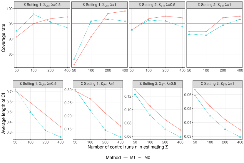
Confidence intervals are an important tool for detection and attribution analyses. It would be desirable if the asymptotic variance in Theorem 2 can be used to construct confidence intervals for the scaling factors. Unfortunately, it has been reported that the confidence intervals for the scaling factors based on have coverage rates lower than, sometimes much lower than, their nominal levels (Li et al., 2019). The under-coverage issue remains for the estimator based on . To give confidence intervals with correct coverage rates, Li et al. (2019) proposed a calibration procedure which enlarges the confidence intervals based on the asymptotic normality of the estimators by an appropriate scale tuned by a parametric bootstrap to achieve the desired coverage rate. We applied this calibration to both M1 and M2 estimators. Figure 2 shows the empirical coverage rates of the 95% confidence intervals after the calibration. The coverage rate of a naive confidence interval could be as low as 70% (not shown). After the calibration, the coverage rates are much closer to the nominal levels. The agreement is better for larger and more structured . The calibrated confidence intervals from M2 are about 10% shorter to those from M1 overall in both settings of true , except for the case of and sample size where the confidence intervals suffer from under-coverage issue..
5 Fingerprinting Mean Temperature Changes
We apply the proposed approach to the detection and attribution analyses of annual mean temperature of 1951–2010 at the global (GL), continental, and subcontinental scales. The continental scale regions are Northern Hemisphere (NH), NH midlatitude between and (NHM), Eurasia (EA), and North America (NA), which were studied in (Zhang et al., 2006). The subcontinental scale regions are Western North American (WNA), Central North American (CNA), Eastern North American (ENA), southern Canada (SCA), and southern Europe (SEU), where the spatio-temporal correlation structure is more likely to hold.
In each regional analysis, we first constructed observation vector from the HadCRUT4 dataset (Morice et al., 2012). The raw data were monthly anomalies of near-surface air temperature on grid-boxes. At each grid-box, each annual mean temperature was computed from monthly temperatures if at least 9 months were available in that year; otherwise, it was considered missing. Then, 5-year averages were computed if no more than 2 annual averages were missing. To reduce the spatial dimension in the analyses, the grid-boxes were aggregated into larger grid-boxes. In particular, the grid-box sizes were for GL and NH, for NH 30-70, for EA, and for NA. For the subcontinent regions, no aggregation was done except for SCA, in which case grid-boxes were used. Details on the longitude, latitude and spatio-temporal steps of each regions after processing can be found in Table 1.
| Acronym | Regions | Longitude | Latitude | Grid size | |||
| (∘E) | (∘N) | () | |||||
| Global and Continental Regions | |||||||
| GL | Global | 180 / 180 | 90 / 90 | 54 | 11 | 572 | |
| NH | Northern Hemisphere | 180 / 180 | 0 / 90 | 27 | 11 | 297 | |
| NHM | Northern Hemisphere to | 180 / 180 | 30 / 70 | 36 | 11 | 396 | |
| EA | Eurasia | 10 / 180 | 30 / 70 | 38 | 11 | 418 | |
| NA | North America | 130 / 50 | 30 / 60 | 48 | 11 | 512 | |
| Subcontinental Regions | |||||||
| WNA | Western North America | 130 / 105 | 30 / 60 | 30 | 11 | 329 | |
| CNA | Central North America | 105 / 85 | 30 / 50 | 16 | 11 | 176 | |
| ENA | Eastern North America | 85 / 50 | 15 / 30 | 21 | 11 | 231 | |
| SCA | Southern Canada | 110 / 10 | 50 / 70 | 20 | 11 | 220 | |
| SEU | South Eupore | 10 / 40 | 35 / 50 | 30 | 11 | 330 | |
Two external forcings, ANT and NAT, were considered. Their fingerprints and were not observed, but their estimates and were averages over and runs from CIMP5 climate model simulations. The missing pattern in was used to mask the simulated runs. The same procedure used to aggregate the grid-boxes and obtain the 5-year averages in preparing was applied to each masked run of each climate model under each forcing. The final estimates and at each grid-box were averages over all available runs under the ANT and the NAT forcings, respectively, centered by the average of the observed annual temperatures over 1961–1990, the same center used by the HadCRUT4 data to obtain the observed anomalies.
Estimation of was based on runs of 60 years constructed from 47 pre-industrial control simulations of various length. The long-term linear trend was removed separately from the control simulations at each grid-box. As the internal climate variation is assumed to be stationary over time, each control run was first split into non-overlapping blocks of 60 years, and then each 60-year block was masked by the same missing pattern as the HadCRUT4 data to create up to 12 5-year averages at each grid-box. The temporal stationarity of variance at each grid implies equal variance over time steps at each observing grid-box, which is commonly incorporated in detection and attribution analyses of climate change (e.g., Hannart, 2016). Both M1 and M2 estimates based on linear and nonlinear shrinkage, respectively, were obtained for comparison. Pooled estimation of the variance at each grid-box was considered in each of the shrinkage estimation to enforce the stationary, grid-box specific variance.

Figure 3 summarizes the GTLS estimates of the scaling factors and for the ANT and NAT forcings, respectively. The estimates from pre-whitening weight matrix and are denoted again as M1 and M2, respectively. The 95% confidence intervals were obtained with the calibration approach of Li et al. (2019). The point estimates from M1 and M2 are similar in all the analysis. The confidence intervals from the M2 method are generally shorter than those from the M1 method in the analyses both at continental and subcontinental scale. More obvious reduction in the confidence interval lengths is observed at the subcontinental scales, e.g., the ANT scaling factor in EA/NA/SCA and the NAT scaling factor in NA/WNA/SCA. This may be explained by that signals at subcontinental scale are weaker and that the error covariance matrix has non-smooth eigenvalues that form some clustering patterns due to weak temporal dependence, as suggested by the simulation study. Although the detection and attribution conclusions based on the confidence intervals remain the same in most cases, the shortened confidence intervals means reduced uncertainty in the estimate of the attributable warming (Jones et al., 2013) and other quantities based on detection and attribution analysis, such as future climate projection and transient climate sensitivity (Li et al., 2019).
6 Discussion
Optimal fingerprinting as the most commonly used method for detection and attribution analyses of climate change has great impact in climate research. Such analyses are the basis for projecting observationally constrained future climate (e.g., Jones et al., 2016) and estimating important properties of the climate system such as climate sensitivity (e.g., Schurer et al., 2018). The original optimality of optimal fingerprinting, which minimizes the uncertainty in the resulting scaling factor estimator, is no longer valid under realistic settings where is not known but estimated. Our method constructs a weight matrix by inverting a nonlinear shrinkage estimator of , which directly minimizes the variation of the resulting scaling factor estimator. This method is more efficient than the current RF practice (Ribes et al., 2013) as evident from the simulation study. Therefore, the lost optimality in fingerprinting is restored to a good extent for practical purposes, which helps to reduce the uncertainty in important quantities such as attributable warming and climate sensitivity.
There are open questions that we have not addressed. It is of interest to further investigate how the asymptotic results under and can guide the RF practice. The temporal and spatial resolution that controls can be tuned in RF practice, which may lead to different efficiencies in inferences and, hence, different results in detection and attribution. Is there an optimal temporal/spatial resolution to obtain the most reliable result? Goodness-of-fit check is an important element in detection and attribution analyses. The classic approach to check the weighted sum of squared residuals against a chi-squared distribution under the assumption of known is not valid when has to be estimated. Can a test be designed, possibly based on parametric bootstrap, to take into account of the uncertainty in regularized estimation of ? These questions merit future research.
Acknowledgements
JY’s research was partially supported by NSF grant DMS 1521730. KC’s research was partially supported by NSF grant IIS 1718798.
Supplementary Materials
A Sufficiency to Assume Orthogonal Covariates
Consider the singular value decomposition of design matrix :
where is a orthogonal matrix, is a matrix with non-negative singular values on the diagonal, and is a orthogonal matrix.
Let and . The columns of are orthogonal. The linear regression can be expressed as
The estimator of is
and the corresponding covariance matrix is
The orthogonality of ensures that and . Therefore, we only need to consider the orthogonal design in the regression model. In other words, we may assume that the columns of the design matrix have columns such that for any .
B Justification of Method M2 in the GLS Case
It is critically important to estimate the covariance matrix precisely as the covariance matrix of depends on . In the estimation of the covariance matrix, an important question is how to quantify the quality of the covariance matrix estimator. We use loss functions to measure the quality of the covariance matrix estimator. For example, one loss function is the Frobenius norm of the bias of the estimator
and another loss function is Stein’s loss
which is the Kullback–Leibler divergence under the normal assumption.
B.1 Minimum Variance Loss Function
Considering the purpose of the fingerprinting, we construct a loss function directly related to the variance of the scaling factor estimator. In other words, we minimize the summation of the variances of the estimated scaling factors
From the random matrix theory (Marc̆enko and Pastur, 1967), we have the following results under the assumption that all limiting forms exist. Consider an random vector whose entries are independent and identically distributed with mean zero, positive variance, and finite 12th moment. Let be a given matrix. Then there exists a constant independent of and x such that (Ledoit and Péché, 2011; Silverstein and Bai, 1995)
or
where is the spectral norm of . In other words, if for some constant , then as ,
Similarly, for two independent random vector x and y,
Now let be an matrix with independent columns. Then, for any matrix with , the matrix
where the righthand side is a matrix of zeroes. In other words, and have the same limit.
In optimal fingerprinting, let be the sample covariance matrix estimated from ensemble runs representing the internal climate variation. Suppose that the eigendecomposition of is , where is the diagonal matrix of the eigenvalues and contains the corresponding eigenvectors. Consider the rotation invariant class of the estimators , where , for a smooth function . Under the same Assumptions 1–3 of the main text, we have both and bounded. Then the assumptions of almost sure convergence are satisfied.
Consider the loss function
Under the orthogonality assumption of , . Therefore, we can consider a loss function with the same limit,
which has the same form as what Ledoit and Wolf (2017b) got. We have, as ,
B.2 Minimum General Variance Loss Function
Instead of considering the trace, we can use the determinant of as the objective loss function. Then the loss function is
It is asymptotically equivalent to loss function
Similar to the minimum variance loss function, we can consider the loss function with the same limiting form:
In other words, as ,
That is, minimizing the limiting forms of two loss functions are asymptotically equivalent to minimize the limiting form of
This concludes the proof of Theorem 1 of the main text.
C Justification of Method M2 in the GTLS Case
C.1 Proofs of Lemma 2 of the Main Text
Proof.
The results are direct extensions of those in Gleser (1981), we only briefly sketch the proof. Consider the observed data matrix which is obtained by binding the columns of and . Under the Assumption 1, 2 and 3, let and , we have
| (C.8) |
which is in the same form of Lemma 3.1 in Gleser (1981). Consider the eigen decomposition of the matrix , where , and the matrix is partitioned as
with matrix . Then following the results of Lemma 3.3 by Gleser (1981), converges to the eigenvectors corresponding to the largest eigenvalues of the limiting matrix of , denoted by . Moreover, we have that there is a nonsingular matrix such that
C.2 Proof of Theorem 2 of the Main Text
Proof.
In the context of general asymptotics, i.e., with fixed ratio, consider the eigendecomposition of matrix , where is the diagonal matrix of eigenvalues, and is the corresponding matrix of eigenvectors. Let
| (C.9) | ||||
Then from Equation (6) of the main text, the generalized total least squares estimator solves equation
where is a dimensional vector. By Taylor’s theorem there exists a series of on the line segment between and for such that
It follows that
where for , is the th element of vector , is the th row vector of and is the th row vector of .
From Assumption 5 in the main text and Equation (C.9), , , and are mutually independent vectors with finite covariance matrices
such that
Then from Lemma 4.1 of Gleser (1981) and Assumption 3 and 4 of the main text,
where .
It remains to show that as ,
| (C.10) |
Consider the derivative of the score function at any value of
Since as and , we have
Thus from the Lemma 2 of the main text and the fact that is a sequence on the line segment between and for , Equation (C.10) holds. With this, we complete the proof of Theorem 2. ∎
C.3 Proof of Theorem 3 of the Main Text
Proof.
Here we sketch the proof in the context of optimal fingerprinting. More rigorous derivations are to be established for the more general setting. As mentioned in Section 3.2 of the main text, without loss of generality, we adjust the Model (2) to make the covariance matrix of the errors in the covariartes and in the response the same. Consider model
where is a normally distributed measurement error vector with mean zero and covariance matrix . Here for the ease of illustration, we consider . Usually in the above model, the magnitudes of fingerprints are comparable to the noise in the sense that the values of and are comparable, i.e., as .
Let , , and . Then the model can be rewritten as
| (C.11) | ||||
| (C.12) |
which is exactly in the form of Models (1)–(2) of the main text with . Then the theoretical results in Section 3.2 of the main text are directly applied to the adjusted model. The coefficient estimations and corresponding variance estimations of the original model can be easily obtained from the results of above adjusted model. That is, in the context of optimal fingerprinting, the original model is equivalent to fit models with relative large magnitudes of fingerprints and small values of true coefficients .
Consider the trace of asymptotic covariance matrix for the estimated coefficient vector in Model given by
| (C.13) | ||||
| (C.14) |
from the Theorem 2 of the main text.
The first term on the right hand side of (C.13) is the same as the loss function proposed in Appendix B.1. In the context of general asymptotics, i.e., with fixed ratio, the first term is equivalent to
as is asymptotically equivalent to for properly defined matrices and (See Appendix B.1).
As for the second term , we need to show that it is dominated by the first term. Given the information on the magnitudes of fingerprints and coefficients from the above illustrations, with appropriate large choice for the value of (which is fairly reasonable in real fingerprinting studies), the small values of can be omitted in the second term. Then the second term can be approximated by . We further note that and . Then we have in the general asymptotics
where as based on the adjustment in Model (C.11). That is, with fairly large value of the number of climate simulations to obtain the estimated fingerprints , the second term on the right hand side of (C.13) can be dominated by the first term, i.e., as we have
for an arbitrary small value with large enough magnitude of in Model (C.11), i.e., large enough number of climate simulations for computing the fingerprints in the original model. Thus the proposed covariance matrix which is the optimal choice regarding the first term in general asymptotics is expected to outperform the linear shrinkage estimator in the sense that
which is consistent with the fact that as the number of climate simulations to estimate the fingerprints becomes larger, the effects of measurement error diminish.
This completes the proof. ∎
D Detailed Results on Simulation Studies
The results of simulation studies in Section 4 of the main text are detailed in Table D.1, Table D.2 and Figure D.1.
| ANT | NAT | ||||||||||||
| N | CB | N | CB | ||||||||||
| size | method | Bias | SD | CIL | CR | CIL | CR | Bias | SD | CIL | CR | CIL | CR |
| Setting 1: ; SNR | |||||||||||||
| 50 | M1 | 0.02 | 19.0 | 0.41 | 69.8 | 0.53 | 82.0 | 0.01 | 57.0 | 1.47 | 78.5 | 1.89 | 89.9 |
| M2 | 0.02 | 17.3 | 0.38 | 69.2 | 0.55 | 84.7 | 0.01 | 49.7 | 1.23 | 76.3 | 1.79 | 92.6 | |
| 100 | M1 | 0.01 | 13.6 | 0.36 | 76.8 | 0.47 | 89.9 | -0.02 | 36.9 | 1.12 | 85.8 | 1.46 | 94.0 |
| M2 | -0.00 | 9.7 | 0.29 | 83.4 | 0.40 | 97.0 | -0.02 | 26.8 | 0.81 | 86.1 | 1.13 | 95.6 | |
| 200 | M1 | 0.00 | 9.0 | 0.30 | 89.4 | 0.39 | 96.2 | -0.01 | 24.4 | 0.87 | 92.4 | 1.08 | 97.5 |
| M2 | -0.00 | 6.7 | 0.23 | 91.3 | 0.26 | 95.4 | -0.01 | 18.7 | 0.64 | 89.1 | 0.76 | 94.8 | |
| 400 | M1 | 0.00 | 6.1 | 0.26 | 93.7 | 0.30 | 96.7 | -0.01 | 18.9 | 0.72 | 93.2 | 0.83 | 97.0 |
| M2 | -0.00 | 5.6 | 0.20 | 93.2 | 0.22 | 94.0 | -0.00 | 16.1 | 0.57 | 92.1 | 0.64 | 94.3 | |
| Setting 1: ; SNR | |||||||||||||
| 50 | M1 | 0.00 | 9.0 | 0.20 | 71.9 | 0.25 | 80.7 | -0.01 | 20.4 | 0.63 | 87.2 | 0.73 | 92.4 |
| M2 | 0.00 | 8.5 | 0.18 | 72.5 | 0.26 | 83.9 | -0.00 | 19.2 | 0.55 | 80.9 | 0.68 | 89.6 | |
| 100 | M1 | 0.00 | 6.6 | 0.18 | 79.8 | 0.23 | 90.7 | -0.01 | 14.8 | 0.51 | 91.0 | 0.59 | 96.2 |
| M2 | 0.00 | 4.5 | 0.14 | 85.6 | 0.19 | 96.5 | -0.01 | 12.0 | 0.38 | 86.9 | 0.46 | 94.6 | |
| 200 | M1 | 0.00 | 4.5 | 0.15 | 88.6 | 0.19 | 95.9 | -0.00 | 10.2 | 0.41 | 95.4 | 0.46 | 97.5 |
| M2 | 0.00 | 3.3 | 0.12 | 92.1 | 0.13 | 95.6 | 0.00 | 8.7 | 0.31 | 93.2 | 0.35 | 95.9 | |
| 400 | M1 | 0.00 | 3.2 | 0.13 | 94.0 | 0.14 | 96.5 | -0.00 | 8.3 | 0.34 | 95.6 | 0.37 | 96.7 |
| M2 | 0.00 | 2.8 | 0.10 | 92.4 | 0.11 | 94.0 | -0.00 | 7.8 | 0.28 | 91.3 | 0.30 | 95.4 | |
| Setting 2: ; SNR | |||||||||||||
| 50 | M1 | -0.00 | 3.2 | 0.10 | 87.7 | 0.11 | 91.8 | 0.00 | 8.7 | 0.33 | 91.8 | 0.39 | 96.7 |
| M2 | 0.00 | 3.1 | 0.09 | 85.6 | 0.11 | 91.0 | 0.00 | 8.5 | 0.30 | 89.9 | 0.35 | 95.1 | |
| 100 | M1 | -0.00 | 2.2 | 0.08 | 93.2 | 0.10 | 96.7 | 0.00 | 7.1 | 0.26 | 91.3 | 0.30 | 95.6 |
| M2 | -0.00 | 2.0 | 0.07 | 91.6 | 0.08 | 95.6 | 0.00 | 7.0 | 0.23 | 87.7 | 0.26 | 91.6 | |
| 200 | M1 | -0.00 | 1.6 | 0.07 | 95.6 | 0.08 | 97.3 | 0.00 | 5.9 | 0.22 | 94.0 | 0.25 | 96.5 |
| M2 | -0.00 | 1.6 | 0.06 | 94.0 | 0.06 | 95.4 | 0.00 | 5.6 | 0.19 | 90.5 | 0.21 | 93.7 | |
| 400 | M1 | -0.00 | 1.5 | 0.06 | 94.8 | 0.06 | 96.5 | 0.00 | 5.1 | 0.19 | 91.0 | 0.21 | 93.7 |
| M2 | -0.00 | 1.4 | 0.05 | 92.4 | 0.05 | 93.5 | -0.00 | 4.8 | 0.17 | 88.8 | 0.18 | 90.7 | |
| Setting 2: ; SNR | |||||||||||||
| 50 | M1 | -0.00 | 1.6 | 0.05 | 84.2 | 0.06 | 90.5 | 0.00 | 4.4 | 0.16 | 93.5 | 0.18 | 94.8 |
| M2 | -0.00 | 1.6 | 0.04 | 80.7 | 0.05 | 89.6 | 0.00 | 4.5 | 0.15 | 90.2 | 0.16 | 91.6 | |
| 100 | M1 | -0.00 | 1.1 | 0.04 | 92.4 | 0.05 | 97.3 | 0.00 | 3.2 | 0.13 | 95.4 | 0.14 | 97.8 |
| M2 | -0.00 | 1.0 | 0.04 | 89.4 | 0.04 | 95.4 | 0.00 | 3.2 | 0.11 | 92.6 | 0.12 | 95.9 | |
| 200 | M1 | -0.00 | 0.8 | 0.03 | 94.0 | 0.04 | 97.0 | 0.00 | 2.8 | 0.11 | 94.8 | 0.12 | 96.7 |
| M2 | 0.00 | 0.7 | 0.03 | 93.7 | 0.03 | 95.4 | 0.00 | 2.7 | 0.10 | 92.6 | 0.10 | 94.6 | |
| 400 | M1 | 0.00 | 0.7 | 0.03 | 96.7 | 0.03 | 97.5 | 0.00 | 2.3 | 0.09 | 95.9 | 0.10 | 97.8 |
| M2 | 0.00 | 0.6 | 0.03 | 95.4 | 0.03 | 95.4 | 0.00 | 2.3 | 0.08 | 92.4 | 0.09 | 94.6 | |
| ANT | NAT | ||||||||||||
| N | CB | N | CB | ||||||||||
| size | method | Bias | SD | CIL | CR | CIL | CR | Bias | SD | CIL | CR | CIL | CR |
| Setting 1: ; SNR | |||||||||||||
| 50 | M1 | 0.00 | 24.6 | 0.53 | 74.9 | 0.71 | 90.7 | -0.00 | 130.9 | 2.08 | 66.8 | 3.07 | 85.8 |
| M2 | 0.00 | 22.8 | 0.47 | 71.9 | 0.72 | 92.6 | 0.05 | 115.2 | 1.77 | 64.9 | 3.22 | 92.1 | |
| 100 | M1 | -0.00 | 17.4 | 0.44 | 82.3 | 0.59 | 95.1 | 0.06 | 97.1 | 1.90 | 70.0 | 2.90 | 90.7 |
| M2 | -0.00 | 11.5 | 0.34 | 86.4 | 0.50 | 98.1 | 0.02 | 53.3 | 1.29 | 76.6 | 2.28 | 94.6 | |
| 200 | M1 | 0.01 | 11.4 | 0.36 | 89.1 | 0.47 | 96.7 | 0.03 | 47.0 | 1.37 | 83.7 | 2.02 | 94.6 |
| M2 | 0.00 | 7.4 | 0.27 | 92.1 | 0.32 | 95.6 | 0.00 | 29.9 | 0.91 | 88.8 | 1.24 | 97.5 | |
| 400 | M1 | 0.00 | 7.5 | 0.30 | 94.3 | 0.35 | 97.3 | 0.02 | 30.5 | 1.09 | 90.5 | 1.41 | 96.2 |
| M2 | 0.00 | 6.5 | 0.23 | 91.8 | 0.25 | 93.7 | 0.01 | 21.3 | 0.79 | 92.4 | 0.95 | 96.2 | |
| Setting 1: ; SNR | |||||||||||||
| 50 | M1 | -0.00 | 11.0 | 0.23 | 69.2 | 0.30 | 81.5 | 0.05 | 37.7 | 0.90 | 76.8 | 1.22 | 87.7 |
| M2 | -0.01 | 10.5 | 0.21 | 69.2 | 0.30 | 83.4 | 0.03 | 32.7 | 0.73 | 72.5 | 1.15 | 92.4 | |
| 100 | M1 | -0.00 | 7.6 | 0.20 | 78.5 | 0.27 | 90.7 | 0.01 | 24.6 | 0.69 | 82.3 | 0.94 | 92.9 |
| M2 | 0.00 | 5.2 | 0.16 | 86.9 | 0.22 | 95.9 | 0.00 | 17.0 | 0.47 | 83.4 | 0.71 | 95.1 | |
| 200 | M1 | -0.00 | 4.7 | 0.17 | 91.0 | 0.21 | 98.4 | -0.00 | 15.0 | 0.50 | 88.8 | 0.66 | 95.4 |
| M2 | -0.00 | 3.4 | 0.13 | 94.6 | 0.14 | 96.5 | -0.01 | 11.5 | 0.36 | 87.2 | 0.45 | 94.0 | |
| 400 | M1 | 0.00 | 3.4 | 0.14 | 97.8 | 0.16 | 99.2 | -0.00 | 11.4 | 0.42 | 90.2 | 0.49 | 95.4 |
| M2 | 0.00 | 2.8 | 0.11 | 95.1 | 0.12 | 95.9 | -0.01 | 9.3 | 0.32 | 89.6 | 0.37 | 92.4 | |
| Setting 2: ; SNR | |||||||||||||
| 50 | M1 | 0.00 | 3.6 | 0.11 | 85.6 | 0.13 | 92.9 | 0.01 | 14.2 | 0.39 | 81.2 | 0.60 | 96.2 |
| M2 | 0.00 | 3.5 | 0.10 | 83.4 | 0.12 | 92.9 | 0.01 | 12.6 | 0.35 | 81.5 | 0.55 | 97.3 | |
| 100 | M1 | -0.00 | 2.5 | 0.09 | 91.8 | 0.11 | 96.7 | -0.00 | 9.0 | 0.30 | 88.0 | 0.40 | 96.7 |
| M2 | -0.00 | 2.3 | 0.08 | 91.6 | 0.09 | 96.2 | -0.00 | 8.1 | 0.27 | 89.1 | 0.34 | 95.1 | |
| 200 | M1 | 0.00 | 1.9 | 0.07 | 94.6 | 0.08 | 97.5 | 0.00 | 6.6 | 0.25 | 93.5 | 0.30 | 97.3 |
| M2 | 0.00 | 1.8 | 0.06 | 94.3 | 0.07 | 95.9 | 0.00 | 5.9 | 0.22 | 92.6 | 0.25 | 96.5 | |
| 400 | M1 | -0.00 | 1.5 | 0.06 | 95.1 | 0.07 | 97.0 | 0.00 | 6.1 | 0.22 | 94.6 | 0.24 | 96.5 |
| M2 | -0.00 | 1.4 | 0.06 | 92.4 | 0.06 | 94.0 | 0.00 | 5.6 | 0.19 | 92.6 | 0.21 | 96.2 | |
| Setting 2: ; SNR | |||||||||||||
| 50 | M1 | -0.00 | 1.7 | 0.05 | 87.2 | 0.06 | 92.4 | 0.00 | 5.4 | 0.18 | 89.4 | 0.23 | 95.1 |
| M2 | -0.00 | 1.6 | 0.05 | 86.4 | 0.06 | 91.6 | 0.00 | 5.3 | 0.16 | 87.2 | 0.21 | 92.9 | |
| 100 | M1 | -0.00 | 1.3 | 0.04 | 89.4 | 0.05 | 92.4 | -0.00 | 3.8 | 0.14 | 92.9 | 0.17 | 96.5 |
| M2 | -0.00 | 1.2 | 0.04 | 86.4 | 0.04 | 91.3 | -0.00 | 3.8 | 0.13 | 91.8 | 0.14 | 93.5 | |
| 200 | M1 | 0.00 | 1.0 | 0.04 | 92.9 | 0.04 | 97.0 | 0.00 | 2.9 | 0.12 | 94.3 | 0.14 | 96.7 |
| M2 | 0.00 | 0.9 | 0.03 | 90.7 | 0.04 | 94.6 | 0.00 | 2.6 | 0.11 | 94.0 | 0.12 | 95.6 | |
| 400 | M1 | -0.00 | 0.7 | 0.03 | 96.5 | 0.03 | 97.5 | -0.00 | 2.6 | 0.10 | 94.6 | 0.12 | 97.0 |
| M2 | -0.00 | 0.7 | 0.03 | 95.1 | 0.03 | 96.5 | -0.00 | 2.5 | 0.09 | 94.3 | 0.10 | 95.6 | |
References
- Allen and Stott (2003) Allen, M. R. and P. A. Stott (2003). Estimating signal amplitudes in optimal fingerprinting, part I: Theory. Climate Dynamics 21, 477–491.
- Allen and Tett (1999) Allen, M. R. and S. F. B. Tett (1999). Checking for model consistency in optimal fingerprinting. Climate Dynamics 15, 419–434.
- Bateman (1954) Bateman, H. (1954). Tables of Integral Transforms, Volume II. New York: McGraw-Hill.
- Bindoff et al. (2013) Bindoff, N. L., P. A. Stott, K. M. AchutaRao, M. R. Allen, N. Gillett, D. Gutzler, K. Hansingo, G. Hegerl, Y. Hu, S. Jain, I. I. Mokhov, J. Overland, J. Perlwitz, R. Sebbari, and X. Zhang (2013). Detection and attribution of climate change: From global to regional. In T. F. Stocker, D. Qin, G.-K. Plattner, M. Tignor, S. K. Allen, J. Boschung, A. Nauels, Y. Xia, V. Bex, and P. M. Midgley (Eds.), Climate Change 2013: The Physical Science Basis. Contribution of Working Group I to the Fifth Assessment Report of the Intergovernmental Panel on Climate Change, Book section 10, pp. 867–952. Cambridge, United Kingdom and New York, NY, USA: Cambridge University Press.
- DelSole et al. (2019) DelSole, T., L. Trenary, X. Yan, and M. K. Tippett (2019). Confidence intervals in optimal fingerprinting. Climate Dynamics 52, 4111–4126.
- Engle et al. (2019) Engle, R. F., O. Ledoit, and M. Wolf (2019). Large dynamic covariance matrices. Journal of Business & Economic Statistics 37, 363–375.
- Fuller (1980) Fuller, W. A. (1980). Properties of some estimators for the errors-in-variables model. Annals of Statistics 8, 407–422.
- Gleser (1981) Gleser, L. J. (1981). Estimation in a multivariate “errors in variables” regression model: Large sample results. Annals of Statistics 9(1), 24–44.
- Hannart (2016) Hannart, A. (2016). Integrated optimal fingerprinting: Method description and illustration. Journal of Climate 29(6), 1977–1998.
- Hannart et al. (2014) Hannart, A., A. Ribes, and P. Naveau (2014). Optimal fingerprinting under multiple sources of uncertainty. Geophysical Research Letters 41(4), 1261–1268.
- Hasselmann (1997) Hasselmann, K. (1997). Multi-pattern fingerprint method for detection and attribution of climate change. Climate Dynamics 13(9), 601–611.
- Hegerl and Zwiers (2011) Hegerl, G. and F. Zwiers (2011). Use of models in detection and attribution of climate change. Wiley Interdisciplinary Reviews: Climate Change 2(4), 570–591.
- Hegerl et al. (2010) Hegerl, G. C., O. Hoegh-Guldberg, G. Casassa, M. P. Hoerling, R. S. Kovats, C. Parmesan, D. W. Pierce, and P. A. Stott (2010). Good practice guidance paper on detection and attribution related to anthropogenic climate change. In T. F. Stocker, C. B. Field, D. Qin, V. Barros, G.-K. Plattner, M. Tignor, P. M. Midgley, and K. L. Ebi (Eds.), Meeting Report of the Intergovernmental Panel on Climate Change Expert Meeting on Detection and Attribution of Anthropogenic Climate Change, Bern, Switzerland. IPCC Working Group I Technical Support Unit, University of Bern.
- Hegerl et al. (1996) Hegerl, G. C., H. von Storch, K. Hasselmann, B. D. Santer, U. Cubasch, and P. D. Jones (1996). Detecting greenhouse-gas-induced climate change with an optimal fingerprint method. Journal of Climate 9(10), 2281–2306.
- Jones et al. (2013) Jones, G. S., P. A. Stott, and N. Christidis (2013). Attribution of observed historical near–surface temperature variations to anthropogenic and natural causes using CMIP5 simulations. Journal of Geophysical Research: Atmospheres 118(10), 4001–4024.
- Jones et al. (2016) Jones, G. S., P. A. Stott, and J. F. B. Mitchell (2016). Uncertainties in the attribution of greenhouse gas warming and implications for climate prediction. Journal of Geophysical Research: Atmospheres 121(12), 6969–6992.
- Ledoit and Péché (2011) Ledoit, O. and S. Péché (2011). Eigenvectors of some large sample covariance matrix ensembles. Probability Theory and Related Fields 150, 233–264.
- Ledoit and Wolf (2004) Ledoit, O. and M. Wolf (2004). A well-conditioned estimator for large-dimensional covariance matrices. Journal of Multivariate Analysis 88(2), 365–411.
- Ledoit and Wolf (2017a) Ledoit, O. and M. Wolf (2017a). Direct nonlinear shrinkage estimation of large-dimensional covariance matrices. Working Paper 264, University of Zurich, Department of Economics.
- Ledoit and Wolf (2017b) Ledoit, O. and M. Wolf (2017b). Nonlinear shrinkage of the covariance matrix for portfolio selection: Markowitz meets Goldilocks. Review of Financial Studies 30(12), 4349–4388.
- Ledoit and Wolf (2018) Ledoit, O. and M. Wolf (2018). Optimal estimation of a large-dimensional covariance matrix under Stein’s loss. Bernoulli 24(4B), 3791–3832.
- Li et al. (2020) Li, Y., K. Chen, and J. Yan (2020). dacc: Detection and Attribution of Climate Change. R package version 0.1-13.
- Li et al. (2019) Li, Y., K. Chen, J. Yan, and X. Zhang (2019). Confidence interval calibration for regularized optimal fingerprinting in detection and attribution of climate change. Technical report, Department of Statistics, University of Connecticut.
- Marc̆enko and Pastur (1967) Marc̆enko, V. and L. A. Pastur (1967). Distribution of eigenvalues for some sets of random matrices. Sbornik: Mathematics 4(1), 457–483.
- Morice et al. (2012) Morice, C. P., J. J. Kennedy, N. A. Rayner, and P. D. Jones (2012). Quantifying uncertainties in global and regional temperature change using an ensemble of observational estimates: The HadCRUT4 data set. Journal of Geophysical Research: Atmospheres 117, D08101.
- Pesta (2013) Pesta, M. (2013). Total least squares and bootstrapping with applications in calibration. Statistics 47(5), 966––991.
- Ribes et al. (2009) Ribes, A., J.-M. Azaïs, and S. Planton (2009). Adaptation of the optimal fingerprint method for climate change detection using a well-conditioned covariance matrix estimate. Climate Dynamics 33(5), 707–722.
- Ribes et al. (2013) Ribes, A., S. Planton, and L. Terray (2013). Application of regularised optimal fingerprinting to attribution. Part I: Method, properties and idealised analysis. Climate Dynamics 41(11-12), 2817–2836.
- Schurer et al. (2018) Schurer, A., G. Hegerl, A. Ribes, D. Polson, C. Morice, and S. Tett (2018). Estimating the transient climate response from observed warming. Journal of Climate 31(20), 8645–8663.
- Silverstein (1995) Silverstein, J. W. (1995). Strong convergence of the empirical distribution of eigenvalues of large-dimensional random matrices. Journal of Multivariate Analysis 55, 331–339.
- Silverstein and Bai (1995) Silverstein, J. W. and Z. Bai (1995). On the empirical distribution of eigenvalues of a class of large-dimensional random matrices. Journal of Multivariate Analysis 54, 175–192.
- Zhang et al. (2006) Zhang, X., F. Zwiers, and P. A. Stott (2006). Multimodel multisignal climate change detection at regional scale. Journal of Climate 19(17), 4294–4307.