Regret Bounds for Gaussian-Process Optimization in Large Domains

Manuel Wüthrich
MPI for Intelligent Systems
Tübingen, Germany
&Bernhard Schölkopf
MPI for Intelligent Systems
Tübingen, Germany
&Andreas Krause
ETH Zurich
Zurich, Switzerland
[email protected]

Abstract

The goal of this paper is to characterize Gaussian-Process optimization in the setting where the function domain is large relative to the number of admissible function evaluations, i.e., where it is impossible to find the global optimum. We provide upper bounds on the suboptimality (Bayesian simple regret) of the solution found by optimization strategies that are closely related to the widely used expected improvement (EI) and upper confidence bound (UCB) algorithms. These regret bounds illuminate the relationship between the number of evaluations, the domain size (i.e. cardinality of finite domains / Lipschitz constant of the covariance function in continuous domains), and the optimality of the retrieved function value. In particular, we show that even when the number of evaluations is far too small to find the global optimum, we can find nontrivial function values (e.g. values that achieve a certain ratio with the optimal value).

1 Introduction

In practice, nonconvex, gradient-free optimization problems arise frequently, for instance when tuning the parameters of an algorithm or optimizing the controller of a physical system (see e.g. Shahriari et al. (2016)) for more concrete examples). Different versions of this problem have been addressed e.g. in the multi-armed-bandit and the Bayesian-optimization literature (which we review below). However, the situation where the number of admissible function evaluations is too small to identify the global optimum has so far received little attention, despite arising frequently in practice. For instance, when optimizing the hyper-parameters of a machine-learning method or the controller-parameters of a physical system, it is typically impossible to explore the domain exhaustively. We take first steps towards a better understanding of this setting through a theoretical analysis based on the adaptive-submodularity framework by Golovin and Krause (2011). It is not the purpose of the present paper to propose a novel algorithm with better performance (we modify the EI and UCB strategies merely to facilitate the proof), but rather to gain an understanding of how GP-optimization performs in the aforementioned setting, as a function of the number of evaluations and the domain size.

As is done typically, we model the uncertainty about the underlying function as a Gaussian Process (GP). The question is how close we can get to the global optimum with $T$ function evaluations, where $T$ is small relative to the domain of the function (i.e., it is impossible to identify the global optimum with high confidence with only $T$ evaluations). As a performance measure, we use the Bayesian simple regret, i.e., the expected difference between the optimal function value and the value attained by the algorithm. For the discrete case with domain size $N$ , we derive a problem-independent regret bound (i.e., it only depends on $T,N$ and is worst-case in terms of the GP prior) for two optimization algorithms that are closely related to the well-known expected improvement (EI, Jones et al. (1998)) and the upper confidence bound (UCB, Auer et al. (2002); Srinivas et al. (2010)) methods. In contrast to related work, our bounds are non-vacuous even when we can only explore a small fraction of the function. We extend this result to continuous domains and show that the resulting bound scales better with the size of the function domain (equivalently, the Lipschitz constant of the covariance function) than related work (Grünewälder et al. (2010)).

1.1 Related Work

The multi-armed bandit literature is closest to the present paper. In the multi-armed bandit problem, the agent faces a row of $N$ slot machines (also called one-armed bandits, hence the name). The agent can decide at each of $T$ rounds which lever (arm) to pull, with the objective of maximizing the payoff. This problem was originally proposed in Robbins (1952) to study the trade-off between exploration and exploitation in a generic and principled way. Since then, this problem has been studied extensively and important theoretical results have been established.

Each of the $N$ arms has an associated reward distribution, with a fixed but unknown mean $F_{n}$ . When pulling arm $n$ at round $t$ , we obtain a payoff $Y_{t}:=F_{n}+E_{n,t}$ where the noise is zero mean $\mathbb{E}[E_{n,t}]=0$ , independent across time steps and arms, and identically distributed for a given arm across time steps. Let us denote the arm pulled at time $t$ by $A_{t}$ . Performance is typically analyzed in terms of the regret, which is defined as the difference between the mean payoff of the optimal arm and the one pulled at time $t$

\displaystyle R_{t}:=\max_{n\in[N]}F_{n}-F_{A_{t}}.

(1)

Here, we are interested in the setting where $E_{n,t}$ is small or even zero and we are allowed to pull only few arms $T<N$ . We classify related work according to the information about the mean $F_{n}$ and the noise $E_{n,t}$ that is available to the agent.

1.1.1 No Prior Information

Traditionally, most authors considered the case where only very basic information about the payoff $F_{n}+E_{n,t}$ is available to the agent, e.g. that its distribution is a member of a given family of distributions or that it takes values in an interval, typically $[0,1]$ .

In a seminal paper, Lai and Robbins (1985) showed that the cumulative regret $\sum_{t\in[T]}R_{t}$ grows at least logarithmically in $T$ and proposed a policy that achieves this rate asymptotically. Later, Auer et al. (2002) proposed an upper confidence bound (UCB) strategy and proved that it achieves logarithmic cumulative regret in $T$ uniformly in time, not just asymptotically. Since then, many related results have been obtained for UCB and other strategies, such as Thompson sampling Agrawal and Goyal (2011); Kaufmann et al. (2012). A number of similar results have also been obtained for the objective of best arm identification Madani et al. (2004); Bubeck et al. (2009); Audibert and Bubeck (2010), where we do not care about the cumulative regret, but only about the lowest regret attained.

However, all of these bounds are nontrivial only when the number of plays is larger than the number of arms $T>N$ . This is not surprising, since no algorithm can be guaranteed to perform well with a low number of plays with such limited information. To see this, consider an example where $F_{i}=1$ and $F_{n}=0\leavevmode\nobreak\ \forall n\neq i$ . Since the agent has no prior information about which is the right arm $i$ , the best it can do is to randomly try out one after the other. Hence it is clear that to obtain meaningful bounds for $T<N$ we need more prior knowledge about the reward distributions of the arms.

1.1.2 Structural Prior Information

In Dani et al. (2008) the authors consider the problem where the mean rewards at each bandit are a linear function of an unknown, $K$ -dimensional vector. However, similarly to the work above, the difficulty addressed in this paper is mainly the noise, i.e. the fact that the same arm does not always yield the same reward. For $E_{n,t}=0$ , the $\mathcal{O}(K)$ cumulative regret bounds derived in this paper are trivial, since with $\mathcal{O}(K)$ evaluations we can simply identify the linear function.

1.1.3 Gaussian Prior

More closely related to our work, a number of authors have considered Gaussian priors. Bull (2011) for instance provides asymptotic convergence rates for the EI strategy with Gaussian-process priors on the unknown function.

Srinivas et al. (2010) propose a UCB algorithm for the Gaussian-process setting. The authors give finite-time bounds on the cumulative regret. However, these bounds are intended for a different setting than the one we consider here: 1) They allow for noisy observations and 2) they are only meaningful if we are allowed to make a sufficient number of evaluations to attain low uncertainty over the entire GP. Please see Appendix B for more details on the second point.

Russo and Van Roy (2014) use a similar analysis to derive bounds for Thompson sampling, which are therefore subject to similar limitations. In contrast, the bounds in Russo and Van Roy (2016) do not depend on the entropy of the entire GP, but rather on the entropy of the optimal action. However, our goal here is to derive bounds that are meaningful even when the optimal action cannot be found, i.e. its entropy remains large.

De Freitas et al. (2012) complement the work in (Srinivas et al., 2010) by providing regret bounds for the setting where the function can be observed without noise. However, these are asymptotic and therefore not applicable to the setting we have in mind.

Similarly to the present paper, Grünewälder et al. (2010) analyze the Bayesian simple regret of GP optimization. They provide a lower and an upper bound on the regret of the optimal policy for GPs on continuous domains with covariance functions that satisfy a continuity assumption. Here, we build on this work and derive a bound with an improved dependence on the Lipschitz constant of the covariance function, i.e., our bound scales better with decreasing length-scales (and, equivalently, larger domains). Unlike (Grünewälder et al., 2010), we also consider GPs on finite domains without any restrictions on the covariance.

1.1.4 Adaptive Submodularity

The adaptive-submodularity framework of Golovin and Krause (2011) is in principle well suited for the kind of analysis we are interested in. However, we will show that the problem at hand is not adaptively submodular, but our proof is inspired by that framework.

2 Problem Definition

2.1 The Finite Case

In this section we specify the type of bandit problem we are interested in more formally. The goal is to learn about a function with domain $\mathcal{A}=[N]$ (we will use $[N]$ to denote the set $\{1,...,N\})$ and co-domain $\mathbb{R}$ . We represent the function as a sequence $F=(F_{n})_{n\in[N]}$ . Our prior belief about the function $F$ is assumed to be Gaussian

\displaystyle F\sim

\displaystyle\mathcal{N}(\mu,\Sigma).

(2)

At each of the $T$ iterations, we pick an action (arm) $A_{t}$ from $[N]$ at which we evaluate the function. After each action, an observation $Y_{t}\in\mathbb{R}$ is returned to the agent

\displaystyle Y_{t}:=F_{A_{t}}.

(3)

Note that here we restrict ourselves to the case where the function can be evaluated without noise.

For convenience, we introduce some additional random variables, based on which the optimization algorithm will pick where to evaluate the function next. We denote the posterior mean and covariance at time $t$ by

	$\displaystyle M_{t}:$	$\displaystyle=\mathbb{E}[F\|A_{:t},Y_{:t}]$		(4)
	$\displaystyle C_{t}:$	$\displaystyle=\mathbb{COV}[F\|A_{:t},Y_{:t}].$		(5)

In addition, we will need the maximum and minimum observations up to time $t$

	$\displaystyle\hat{Y}_{t}:$	$\displaystyle=\max_{k\in[t]}Y_{k}\quad\forall t\in\{1,..,T\}$		(6)
	$\displaystyle\check{Y}_{t}:$	$\displaystyle=\min_{k\in[t]}Y_{k}\quad\forall t\in\{1,..,T\}.$		(7)

Furthermore, we will make statements about the difference between the smallest and the largest observed value

\displaystyle\hat{\check{Y}}_{t}:

\displaystyle=\hat{Y}_{t}-\check{Y}_{t}\quad\forall t\in\{1,..,T\}.

(8)

Finally, for notational convenience we define

\displaystyle\hat{Y},\check{Y},\hat{\check{Y}}:

\displaystyle=\hat{Y}_{T},\check{Y}_{T},\hat{\check{Y}}_{T}.

(9)

Analogously, let us define the function minimum $\check{F}:=\min_{n\in[N]}F_{n}$ , maximum $\hat{F}:=\max_{n\in[N]}F_{n}$ and difference $\hat{\check{F}}:=\hat{F}-\check{F}$ .

2.1.1 Problem Instances

A problem instance is defined by the tuple $(N,T,\mu,\Sigma)$ , i.e. the domain size $N\in\mathbb{N}_{>0}$ , the number of rounds $T\in\mathbb{N}_{>0}$ and the prior 2 with mean $\mu\in\mathbb{R}^{N}$ and covariance $\Sigma\in\mathbb{S}_{+}^{n}$ , where we use $\mathbb{S}_{+}^{n}$ to denote the set of positive semidefinite matrices of size $n$ .

2.2 The Continuous Case

The definitions in the continuous case are analogous. A problem instance here is defined by $(\mathcal{A},T,\mu,k)$ , i.e. the function domain $\mathcal{A}$ , the number of rounds $T\in\mathbb{N}_{>0}$ , a mean function $\mu:\mathcal{A}\to\mathbb{R}$ and a positive semi-definite kernel $k:\mathcal{A}^{2}\to\mathbb{R}$ .

3 Results

In this section we provide bounds on the Bayesian simple regret that hold for the two different optimization algorithms we describe in the following.

3.1 Optimization Algorithms

Two of the most widely used GP-optimization algorithms are the expected improvement (EI) (Jones et al. (1998)) and the upper confidence bound (UCB) (Auer et al. (2002); Srinivas et al. (2010)) methods. In the following, we define two optimization policies that are closely related:

Definition 1.

The expected improvement Bull (2011) is defined as

\displaystyle\operatorname*{ei}(\tau):

\displaystyle=\int_{-\infty}^{\infty}\max\{x-\tau,0\}\mathcal{N}(x)dx=\mathcal{N}(\tau)-\tau\Phi^{c}(\tau)

(10)

where $\mathcal{N}$ is the standard normal density function and $\Phi^{c}$ is the complementary cumulative density function of a standard normal distribution. Furthermore, we use the notation

\displaystyle\operatorname*{ei}(\tau|\mu,\sigma)

\displaystyle=\sigma\operatorname*{ei}\left(\frac{\tau-\mu}{\sigma}\right)=\int_{-\infty}^{\infty}\max\{x-\tau,0\}\mathcal{N}(x|\mu,\sigma)dx.

(11)

Definition 2 (EI2).

An agent follows the EI2 strategy when it picks its actions according to

\displaystyle A_{t+1}

\displaystyle=\operatorname*{argmax}_{n\in[N]}\max\left\{\operatorname*{ei}\left(\hat{Y}_{t}|M_{t}^{n},\sqrt{C_{t}^{nn}}\right),\operatorname*{ei}\left(-\check{Y}_{t}|-M_{t}^{n},\sqrt{C_{t}^{nn}}\right)\right\}

(12)

with the expected improvement $\operatorname*{ei}$ as defined in Definition 1.

Definition 3 (UCB2).

An agent follows the UCB2 strategy when it picks its actions according to

\displaystyle A_{t+1}

\displaystyle=\operatorname*{argmax}_{n\in[N]}\max\left\{-\hat{Y}_{t}+M_{t}^{n}+\sqrt{C_{t}^{nn}2\log N},\check{Y}_{t}-M_{t}^{n}+\sqrt{C_{t}^{nn}2\log N}\right\}.

(13)

The main difference to the standard versions of these methods (see Definition 6 and Definition 7) is that the algorithms here are symmetrical in the sense that they are invariant to flipping the sign of the GP. They maximize and minimize at the same time by picking the point which we expect to either increase the observed maximum or decrease the observed minimum the most. This symmetry is important for our proof, whether the same bound also holds for following the standard, one-sided EI or UCB strategies is an open question, we discuss this point in detail in Section 4.

3.2 Upper Bound on the Bayesian Simple Regret for the Extremization Problem

Here, we provide a regret bound for function extremization (i.e. the goal is to find both the minimum and the maximum) from which the regret bound for function maximization will follow straightforwardly. Note that the bound is problem-independent in the sense that it does not depend on the prior $(\mu,\Sigma)$ .

Theorem 1.

For any instance $(N,T,\mu,\Sigma)$ of the problem defined in Section 2.1 with $N\geq T\geq 500$ , if we follow either the EI2 (Definition 2) or the UCB2 (Definition 3) strategy, we have

\frac{\mathbb{E}\left[\hat{\check{F}}\right]-\mathbb{E}\left[\hat{\check{Y}}\right]}{\mathbb{E}\left[\hat{\check{F}}\right]}\leq 1-\left(1-T^{-\frac{1}{2\sqrt{\pi}}}\right)\sqrt{\frac{\log(T)-\log\left(3\log^{\frac{3}{2}}(T)\right)}{\log(N)}}.

(14)

This guarantees that the expected difference between the maximum and minimum retrieved function value achieves a certain ratio with respect to the expected difference between the global maximum and the global minimum.

Proof.

The full proof can be found in the supplementary material in Appendix G, here we only give an outline. The proof is inspired by the adaptive submodularity framework by Golovin and Krause (2011). The problem at hand can be understood as finding the policy (optimization algorithm) which maximizes an expected utility. Finding this optimal policy would require solving a partially observable Markov decision process (POMDP), which is intractable in most relevant situations. Instead, a common approach is to use a greedy policy which maximizes the expected single-step increase in utility at each time step $t$ , which is in our case

\displaystyle A_{t+1}=\operatorname*{argmax}_{a}\left(\mathbb{E}\left[\hat{Y}_{t+1}-\check{Y}_{t+1}|A_{t+1}=a,A_{:t},Y_{:t}\right]-\mathbb{E}\left[\hat{Y}_{t}-\check{Y}_{t}|A_{:t},Y_{:t}\right]\right).

(15)

This corresponds to the EI2 (Definition 2) strategy. The task now is to show that the greedy policy will not perform much worse than the optimal policy. Golovin and Krause (2011) show that this holds for problems that are adaptively submodular (among some other conditions). In the present problem, we can roughly translate this condition to: The progress we make at a given time step has to be proportional to how far the current best value is from the global optimum. While our problem is not adaptively submodular (see Appendix A), we show that a similar condition holds (which leads to similar guarantees). ∎

3.3 Upper and Lower Bound on the Bayesian Simple Regret for the Maximization Problem

For maximization, the goal is to minimize the Bayesian simple regret, i.e. the expected difference between the globally maximal function value and the best value found by the optimization algorithm

\mathbb{E}[\hat{F}]-\mathbb{E}[\hat{Y}].

(16)

As is often done in the literature (see e.g. Srinivas et al. (2010)), we restrict ourselves here to centered GPs (i.e. zero prior mean; naturally, the mean will change during the optimization). To be invariant to scaling of the prior distribution, we normalize the regret with the expected global maximum:

\text{normreg}:=\frac{\mathbb{E}\left[\hat{F}\right]-\mathbb{E}\left[\hat{Y}\right]}{\mathbb{E}\left[\hat{F}\right]}.

(17)

3.3.1 Upper Regret Bound for the EI2 and UCB2 Policies

We obtain the following upper bound on this normalized Bayesian simple regret:

Corollary 1.

For any instance $(N,T,\mu,\Sigma)$ of the problem defined in Section 2.1 with zero mean $\mu_{n}=0\leavevmode\nobreak\ \forall n$ and $N\geq T\geq 500$ , if we follow either the EI2 (Definition 2) or the UCB2 (Definition 3) strategy, we have

\operatorname*{normreg}\leq 1-\left(1-T^{-\frac{1}{2\sqrt{\pi}}}\right)\sqrt{\frac{\log(T)-\log\left(3\log^{\frac{3}{2}}(T)\right)}{\log(N)}}.

(18)

This implies a bound on the ratio between the expected maximum found by the algorithm and the expected global maximum.

Proof.

The Gaussian prior is symmetric about $0$ , as the mean is $0$ everywhere (i.e. the probability density satisfies $p(F=f)=p(F=-f)\leavevmode\nobreak\ \forall f$ ). Since also both the EI2 and the UCB2 policies are symmetric, we have $\mathbb{E}\left[\hat{F}\right]=-\mathbb{E}\left[\check{F}\right]$ and hence

\mathbb{E}\left[\hat{\check{F}}\right]=\mathbb{E}\left[\hat{F}\right]-\mathbb{E}\left[\check{F}\right]=2\mathbb{E}\left[\hat{F}\right]

(19)

and similarly $\mathbb{E}\left[\hat{\check{Y}}\right]=2\mathbb{E}\left[\hat{Y}\right]$ . Substituting this in Theorem 1, Corollary 1 follows.∎

In Figure 2, we plot this bound, and we observe that we obtain nontrivial regret bounds even when evaluating the function only at a small fraction of its domain.

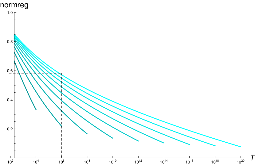
Refer to caption — Figure 1: The upper bound on the regret from Corollary 1 as a function of the number of evaluations $T$ . Each curve corresponds to a different domain size $N$ and is plotted for $T\in\{500,...,N\}$ , hence $N$ can be read from the end point of each curve.

For instance, if we pick the curve that corresponds to $N=10^{20}$ (the rightmost curve), and we choose $T=10^{6}$ , we achieve a regret of about $0.6$ , as indicated in the figure. This means that we can expect to find a function value of about $40\%$ of the expected global maximum by evaluating the function at only a fraction of $10^{-14}$ of its domain, and this holds for any prior covariance $\Sigma$ .

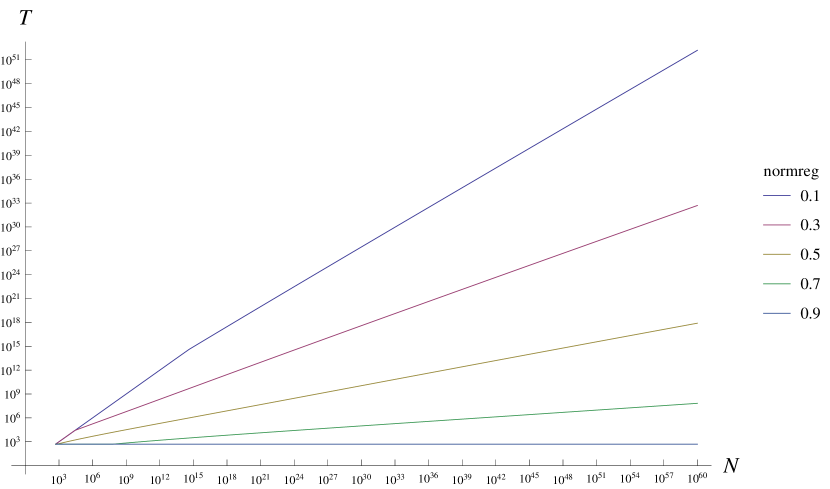
In Figure 2, we plot the upper bound on the required number of evaluations $T$ , implied by Corollary 1, as a function of the domain size $N$ . We observe that $T$ seems to scale polynomially with $N$ (i.e. linearly in log space) with an order that depends on the regret we want to achieve. Indeed, it is easy to see from Corollary 1 that $\forall\epsilon>0\leavevmode\nobreak\ \exists K:\forall N\geq T\geq K:$

\text{normreg}\leq 1-\frac{\sqrt{\log T}}{\sqrt{\log N}}+\epsilon

(20)

which implies that $\forall\epsilon>0\leavevmode\nobreak\ \exists K:\forall N\geq T\geq K:$

T\leq N^{(1-\text{normreg}+\epsilon)^{2}}.

(21)

This means for instance that, if we accept to achieve only $20\%$ of the global maximum, the required number of evaluations grows very slowly with about $T\approx N^{1/25}$ , but still polynomially.

3.3.2 Lower Regret Bound for the Optimal Policy

The upper bound from Corollary 1 is tight, as we can see by comparing 20 to the following result:

Lemma 1 (Lower Bound).

For the instance of the problem defined in Section 2.1 with $\mu=\mathbf{0}$ and $\Sigma=\mathbf{I}$ , the following lower bound on the regret holds for the optimal strategy: $\forall\epsilon>0\leavevmode\nobreak\ \exists K:\forall N\geq T\geq K:$

\operatorname*{normreg}\geq 1-\frac{\sqrt{\log T}}{\sqrt{\log N}}-\epsilon.

(22)

Proof.

Here, sampling without replacement is an optimal strategy, which yields the bound above, see Appendix I for the full proof. ∎

It follows from Lemma 1 that $\forall\epsilon>0\leavevmode\nobreak\ \exists K:\forall N\geq T\geq K:$

T\geq N^{(1-\text{normreg}-\epsilon)^{2}}.

(23)

Hence, for a given regret, the required number of evaluations $T$ grows polynomially in the domain size $N$ , even for the optimal policy, albeit with low degree. This means that if the domain size grows exponentially in the problem dimension, we will inherit this exponential growth also for the necessary number of evaluations. However, since our bounds are problem independent and hence worst-case in terms of the prior covariance $\Sigma$ , this result does not exclude the possibility that for certain covariances we might be able to obtain polynomial scaling of the required number of evaluations in the dimension of the problem.

3.3.3 Lower Regret Bound for Prior-Independent Policies

It is important to note that a uniform random policy will not achieve the bound from Corollary 1 in general. In fact, despite the bound from Corollary 1 being independent of the prior $(\mu,\Sigma)$ , it cannot be achieved by any policy that is independent of the prior:

Lemma 2.

For any optimization policy which does not depend on the prior $(\mu,\Sigma)$ , there exists an instance of the problem defined in Section 2.1 where

\operatorname*{normreg}\geq 1-\frac{T}{N},

(24)

which is clearly worse for $T\ll N$ than the bound in Corollary 1.

Proof.

Suppose we construct a function that is zero everywhere except in one location. Since the policy has no knowledge of that location, it is possible to place it such that the policy will perform no better than random selection, which yields the regret above. See Appendix J for the full proof. ∎

3.4 Extension to Continuous Domains

For finite domains, we looked at the setting where the cardinality of the domain $N$ is much larger than the number of admissible evaluations $T$ . The notion of domain size is less obvious in the continuous case, in the following we clarify this point before we discuss the results.

3.4.1 Problem Setting

In the continuous setting, we characterize the GP by $L_{k}$ and $\sigma$ , which are properties of the kernel $k$ :

	$\displaystyle\|k(x,x)-k(x,y)\|$	$\displaystyle\leq L_{k}\left\\|x-y\right\\|_{\infty}\quad\forall x,y\in\mathcal{A}$		(25)
	$\displaystyle k(x,x)$	$\displaystyle\leq\sigma^{2}\quad\forall x\in\mathcal{A}$		(26)

where $\mathcal{A}$ is the $D$ -dimensional unit cube (note that to use a domain other than the unit cube we can simply rescale). The setting we are interested in is

T\ll\left(\frac{L_{k}}{2\sigma^{2}}\right)^{D}=:m(L_{k},\sigma,D).

(27)

As we discuss in more detail in Appendix C, $m(L_{k},\sigma,D)$ corresponds to the number of points we would require to cover the domain such that we could acquire nonzero information about any point in the domain. Naturally, to guarantee that we can find the global optimum we would require at least that number of evaluations $T$ . Here, in contrast, we consider the setting where $T$ is much smaller and only a small fraction of the GP can be explored.

3.4.2 Results

Here, we adapt Corollary 1 to continuous domains. The bound we propose in the following is based on a result from (Grünewälder et al., 2010), which states that for a centered Gaussian Process $\left(G_{a}\right){}_{a\in\mathcal{A}}$ with domain $\mathcal{A}$ being the $D$ -dimensional unit cube and a Lipschitz-continuous kernel $k$

\left|k(x,x)-k(x,y)\right|\leq L_{k}\left\|x-y\right\|_{\infty}\quad\forall x,y\in\mathcal{A},

(28)

the regret of the optimal policy is bounded by

\displaystyle\mathbb{E}\left[\sup_{a\in\mathcal{A}}G(a)-\hat{Y}\right]

\displaystyle\leq\sqrt{\frac{2L_{k}}{\left\lfloor T^{1/D}\right\rfloor}}\left(2\sqrt{\log\left(2T\right)}+15\sqrt{D}\right).

(29)

Note that Grünewälder et al. (2010) state the bound for the more general case of Hölder-continuous functions, for simplicity of exposition we limit ourselves here to the case of Lipschitz-continuous kernels. Grünewälder et al. (2010) complement this bound with a matching lower bound (up to log factors). However, as we shall see, we can improve substantially on this bound in terms of its dependence on the Lipschitz constant $L_{k}$ if we assume that the variance is bounded, i.e., $k(x,x)\leq\sigma^{2}$ . This is particularly relevant for GPs with short length scales (or, equivalently, large domains) and hence large $L_{k}$ .

Interestingly, Grünewälder et al. (2010) obtain 29 using a policy that selects the actions a priori (by placing them on a grid), without any feedback from the observations made. Here, we will refine 29 by using this strategy for preselecting a large set of admissible actions offline and then selecting actions from this set using EI2 (Definition 2) or UCB2 (Definition 3) online. A reasoning along these lines yields the following bound:

Theorem 2.

For any centered Gaussian Process $\left(G_{a}\right){}_{a\in\mathcal{A}}$ , where $\mathcal{A}$ is the $D$ -dimensional unit cube, with kernel $k$ such that

	$\displaystyle\left\|k(x,x)-k(x,y)\right\|$	$\displaystyle\leq L_{k}\left\\|x-y\right\\|_{\infty}\quad\forall x,y\in\mathcal{A}$		(30)
	$\displaystyle\sqrt{k(x,x)}$	$\displaystyle\leq\sigma\quad\forall x\in\mathcal{A}$		(31)

we obtain the following bound on the regret, if we follow the EI2 (Definition 2) or the UCB2 (Definition 3) strategy:

	$\displaystyle\mathbb{E}\left[\sup_{a\in\mathcal{A}}G(a)-\hat{Y}\right]\leq\sqrt{\frac{2\log(L_{k})}{T^{1/D}}}\left(2\sqrt{\log\left(2\left\lceil\frac{L_{k}}{\log(L_{k})}T^{1/D}\right\rceil^{D}\right)}+15\sqrt{D}\right)+$
	$\displaystyle\quad\quad\quad\quad\quad\sqrt{2}\sigma\left(\sqrt{D\log\left(\left\lceil\frac{L_{k}}{\log(L_{k})}T^{1/D}\right\rceil\right)}-\left(1-T^{-\frac{1}{2\sqrt{\pi}}}\right)\sqrt{\log\left(\frac{T}{3\log^{\frac{3}{2}}(T)}\right)}\right).$		(32)

This bound also holds when restricting EI2 or UCB2 to a uniform grid on the domain $\mathcal{A}$ , where each side is divided into $\left\lceil\frac{L_{k}}{\log(L_{k})}T^{1/D}\right\rceil$ segments. Finally, this bound converges to $0$ as $T\to\infty$ .

Proof.

The idea here is to pre-select a set of $N$ points at locations $X_{1:N}$ on a grid and then sub-select points from this set during runtime using EI2 (Definition 2) or UCB2 (Definition 3). We bound the regret of this strategy by combining Theorem 1 with the main result from (Grünewälder et al., 2010), the full proof can be found in Appendix K. ∎

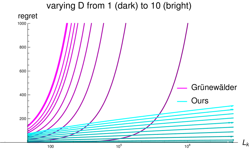
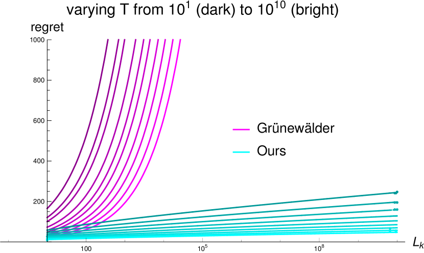
The important point to note here is that in Theorem 2 the bound grows logarithmically in $L_{k}$ , as opposed to the bound 29 from Grünewälder et al. (2010), which grows with $\sqrt{L_{k}}$ . This means that for Gaussian Processes with high $L_{k}$ , i.e. high variability, 32 is much lower than 29 (note that cuboid domains $\mathcal{A}$ can be rescaled to the unit cube by adapting the Lipschitz constant $L_{k}$ accordingly, hence a large domain is equivalent to a large Lipschitz constant). This allows for meaningful bounds even when the number of allowed evaluations is small relative to the domain-size of the function. We illustrate this in Figure 3. Consider for instance the case of $L_{k}=10^{5},\sigma=1,D=2,T=10^{5}$ , where the number of evaluations is far too low to explore the GP ( $T=10^{5}\ll m(L_{k},\sigma,D)=2.5\times 10^{9}$ ). We see from Figure 3(a) that our regret bounds (second-darkest cyan) remain low while the ones from Grünewälder et al. (2010) (second-darkest magenta) explode.

Theorem 2 also provides another insight: To allow for straightforward optimization of the acquisition function (e.g. EI, UCB), the domain is often discretized in practical Bayesian optimization. Theorem 2 tells us how fine this discretization should be to still achieve performance guarantees.

4 Relation to Standard EI and UCB

An empirical comparison (Appendix F) indicates EI2/UCB2 require more evaluations than EI/UCB to attain a given regret, but not more than twice as many. This matches our intuition: We would expect standard EI/UCB to perform better because i) any given step, evaluating at a potential maximizer instead of a minimizer will clearly lead to a larger immediate reduction in expected regret and ii) we would not expect an evaluation at a potential minimizer to provide any more useful information than an evaluation at a potential maximizer. Further, we would not expect EI2/UCB2 to perform much worse because a substantial fraction of its evaluations (in expectation half, for a centered GP) will be maximizations.

If we could prove that EI/UCB performs better than EI2/UCB2 for maximization, this would imply that the regret bounds presented above apply to EI/UCB. Unfortunately, proving this formally appears to be nontrivial. Nevertheless, we are able to give weaker regret bounds for standard EI/UCB which we discuss in the following.

4.1 Upper Bound on the Bayesian Simple Regret for Standard EI and UCB

Let us now consider the standard, one-sided versions of EI (Definition 6) and UCB (Definition 7), which are identical to EI2 (Definition 2) and UCB2 (Definition 3) except that we drop the second term in the $\max$ . We obtain the following version of Theorem 1:

Theorem 3.

For any instance $(N,T,\mu,\Sigma)$ of the problem defined in Section 2.1 with $N\geq T\geq 500$ , if we follow either the EI (Definition 6) or the UCB strategy (Definition 7) we have

\frac{\mathbb{E}\left[\hat{\check{F}}\right]-\mathbb{E}\left[\boldsymbol{\hat{Y}-\check{F}}\right]}{\mathbb{E}\left[\hat{\check{F}}\right]}\leq 1-\left(1-T^{-\frac{1}{2\sqrt{\pi}}}\right)\sqrt{\frac{\log(T)-\log\left(3\log^{\frac{3}{2}}(T)\right)}{\log(N)}}.

(33)

Proof.

The proof is very similar to the one of Theorem 1 and can be found in Appendix H. ∎

Note that we marked the changes in bold. Now, instead of a guarantee on $\hat{\check{Y}}$ , we provide a guarantee on $\hat{Y}-\check{F}$ , i.e. the difference between the best obtained value and the function minimum. We can then derive from that a version of Corollary 1:

Corollary 2.

For any instance $(N,T,\mu,\Sigma)$ of the problem defined in Section 2.1 with zero mean $\mu_{n}=0\leavevmode\nobreak\ \forall n$ and $N\geq T\geq 500$ , if we follow either standard EI (Definition 6) or UCB strategy (Definition 7), we have

normreg\leq\boldsymbol{2}\left(1-\left(1-T^{-\frac{1}{2\sqrt{\pi}}}\right)\sqrt{\frac{\log(T)-\log\left(3\log^{\frac{3}{2}}(T)\right)}{\log(N)}}\right).

(34)

Proof.

The proof is analogous to the one of Corollary 1.

∎

The important thing to note here is the appearance of the factor 2 in the bound. This means that asymptotically we have

\text{normreg}\leq\boldsymbol{2}\left(1-\frac{\sqrt{\log T}}{\sqrt{\log N}}\right)+\epsilon

(35)

and

T\leq N^{(1-\text{normreg}/\boldsymbol{2}+\epsilon)}

(36)

which is weaker compared to 20 and 21. We believe that this gap is not due to EI/UCB actually performing worse than EI2/UCB2, but rather an artifact of the proof.

5 Limitations

While we believe that the results above are insightful, there are a number of limitations one should be aware of:

As discussed in Section 4, the regret bounds we derive for standard EI and UCB are weaker than the ones for EI2 and UCB2, despite the intuition and empirical evidence that EI/UCB most likely perform no worse for maximization than EI2/UCB2. It would be interesting to close this gap.

Another limitation is that the bounds only hold for the noise-free setting. We believe that this limitation is acceptable because the problem of noisy observations is mostly orthogonal to the problem studied herein. Furthermore, the naive solution of reducing the noise by evaluating multiple times at each point leads to qualitatively similar regret bounds, see Appendix D for a more detailed discussion.

Further, the bounds from Corollary 1, Theorem 2, and Corollary 2 only hold for zero prior mean (equivalently, constant prior mean). This assumption is not uncommon in the GP optimization literature (see e.g. Srinivas et al. (2010)) but it may be limiting if one has prior knowledge about where good function values lie. It is likely possible to extend the results in this article to arbitrary prior means.

Finally, there are limitations that hold generally for the GP optimization literature: 1) In a naive implementation, the computational cost is cubic in the number of evaluations $T$ and 2) the assumption that the true function is drawn from a Gaussian Process is typically not realistic and only made for analytical convenience. It is hence not clear whether the relations we uncovered herein apply to realistic optimization settings or if they are mostly an artifact of the GP assumption.

Summarizing, it is clear that the results in the present paper have little direct practical relevance. Instead, the intention is to develop a theoretical understanding of the problem setting.

6 Conclusion

We have characterized GP optimization in the setting where finding the global optimum is impossible because the number of evaluations is too small with respect to the domain size. We derived regret-bounds for the finite-arm setting which are independent of the prior covariance, and we showed that they are tight. Further, we derived regret-bounds for GP optimization in continuous domains that depend on the Lipschitz constant of the covariance function and the maximum variance. In contrast to previous work, our bounds are non-vacuous even when the domain size is very large relative to the number of evaluations. Therefore, they provide novel insights into the performance of GP optimization in this challenging setting. In particular, they show that even when the number of evaluations is far too small to find the global optimum, we can find nontrivial function values (e.g. values that achieve a certain ratio with the optimal value).

References

Agrawal and Goyal [2011] Shipra Agrawal and Navin Goyal. Analysis of thompson sampling for the multi-armed bandit problem. CoRR, abs/1111.1797, 2011. URL http://arxiv.org/abs/1111.1797.
Audibert and Bubeck [2010] Jean-Yves Audibert and Sébastien Bubeck. Best Arm Identification in Multi-Armed Bandits. In COLT - 23th Conference on Learning Theory - 2010, page 13 p., Haifa, Israel, June 2010. URL https://hal-enpc.archives-ouvertes.fr/hal-00654404.
Auer et al. [2002] Peter Auer, Nicolò Cesa-Bianchi, and Paul Fischer. Finite-time analysis of the multiarmed bandit problem. Mach. Learn., 47(2-3):235–256, May 2002. ISSN 0885-6125. doi: 10.1023/A:1013689704352. URL https://doi.org/10.1023/A:1013689704352.
Bubeck et al. [2009] Sébastien Bubeck, Rémi Munos, and Gilles Stoltz. Pure exploration in multi-armed bandits problems. In Proceedings of the 20th International Conference on Algorithmic Learning Theory, ALT’09, pages 23–37, Berlin, Heidelberg, 2009. Springer-Verlag. ISBN 3-642-04413-1, 978-3-642-04413-7. URL http://dl.acm.org/citation.cfm?id=1813231.1813240.
Bull [2011] Adam D. Bull. Convergence rates of efficient global optimization algorithms. Journal of Machine Learning Research, 12:2879–2904, 2011. URL http://dblp.uni-trier.de/db/journals/jmlr/jmlr12.html#Bull11.
Dani et al. [2008] Varsha Dani, Thomas P. Hayes, and Sham M. Kakade. Stochastic linear optimization under bandit feedback. In In submission, 2008.
De Freitas et al. [2012] Nando De Freitas, Alex J. Smola, and Masrour Zoghi. Exponential regret bounds for gaussian process bandits with deterministic observations. In Proceedings of the 29th International Coference on International Conference on Machine Learning, ICML’12, pages 955–962, USA, 2012. Omnipress. ISBN 978-1-4503-1285-1. URL http://dl.acm.org/citation.cfm?id=3042573.3042697.
Golovin and Krause [2011] Daniel Golovin and Andreas Krause. Adaptive submodularity: Theory and applications in active learning and stochastic optimization. Journal of Artificial Intelligence Research (JAIR), 42:427–486, 2011.
GPy [since 2012] GPy. GPy: A gaussian process framework in python. http://github.com/SheffieldML/GPy, since 2012.
Grünewälder et al. [2010] Steffen Grünewälder, Jean-yves Audibert, Manfred Opper, and John Shawe-Taylor. Regret Bounds for Gaussian Process Bandit Problems. In Yee Whye Teh and Mike Titterington, editors, Proceedings of the Thirteenth International Conference on Artificial Intelligence and Statistics, volume 9 of Proceedings of Machine Learning Research, pages 273–280, Chia Laguna Resort, Sardinia, Italy, 2010. PMLR.
Jones et al. [1998] Donald R. Jones, Matthias Schonlau, and William J. Welch. Efficient global optimization of expensive black-box functions. Journal of Global Optimization, 13(4):455–492, Dec 1998. ISSN 1573-2916. doi: 10.1023/A:1008306431147. URL https://doi.org/10.1023/A:1008306431147.
Kaufmann et al. [2012] Emilie Kaufmann, Nathaniel Korda, and Rémi Munos. Thompson sampling: An asymptotically optimal finite-time analysis. In Proceedings of the 23rd International Conference on Algorithmic Learning Theory, ALT’12, pages 199–213, Berlin, Heidelberg, 2012. Springer-Verlag. ISBN 978-3-642-34105-2. doi: 10.1007/978-3-642-34106-9˙18. URL http://dx.doi.org/10.1007/978-3-642-34106-9_18.
Krause and Golovin [2014] Andreas Krause and Daniel Golovin. Submodular function maximization. In Tractability: Practical Approaches to Hard Problems. Cambridge University Press, February 2014.
Lai and Robbins [1985] T.L Lai and Herbert Robbins. Asymptotically efficient adaptive allocation rules. Adv. Appl. Math., 6(1):4–22, March 1985. ISSN 0196-8858. doi: 10.1016/0196-8858(85)90002-8. URL http://dx.doi.org/10.1016/0196-8858(85)90002-8.
Madani et al. [2004] Omid Madani, Daniel J. Lizotte, and Russell Greiner. Active model selection. In Proceedings of the 20th Conference on Uncertainty in Artificial Intelligence, UAI ’04, pages 357–365, Arlington, Virginia, United States, 2004. AUAI Press. ISBN 0-9749039-0-6. URL http://dl.acm.org/citation.cfm?id=1036843.1036887.
Massart [2007] Pascal Massart. Concentration Inequalities and Model Selection. Springer, June 2007. URL https://market.android.com/details?id=book-LmErAAAAYAAJ.
Nemhauser et al. [1978] G. L. Nemhauser, L. A. Wolsey, and M. L. Fisher. An analysis of approximations for maximizing submodular set functions—i. Mathematical Programming, 14(1):265–294, 1978.
Pedregosa et al. [2011] Fabian Pedregosa, Gaël Varoquaux, Alexandre Gramfort, Vincent Michel, Bertrand Thirion, Olivier Grisel, Mathieu Blondel, Peter Prettenhofer, Ron Weiss, Vincent Dubourg, Jake Vanderplas, Alexandre Passos, David Cournapeau, Matthieu Brucher, Matthieu Perrot, and Édouard Duchesnay. Scikit-learn: Machine Learning in Python. Journal of machine learning research: JMLR, 12(null):2825–2830, November 2011. URL https://dl.acm.org/doi/10.5555/1953048.2078195.
Robbins [1952] Herbert Robbins. Some aspects of the sequential design of experiments. Bulletin of the American Mathematical Society, 58(5):527–535, 1952. URL http://www.projecteuclid.org/DPubS/Repository/1.0/Disseminate?view=body&id=pdf_1&handle=euclid.bams/1183517370.
Russo and Van Roy [2016] D Russo and B Van Roy. An information-theoretic analysis of thompson sampling. Journal of machine learning research: JMLR, 2016.
Russo and Van Roy [2014] Daniel Russo and Benjamin Van Roy. Learning to Optimize via Posterior Sampling. Mathematics of Operations Research, 39(4):1221–1243, April 2014.
Shahriari et al. [2016] B. Shahriari, K. Swersky, Z. Wang, R. P. Adams, and N. de Freitas. Taking the human out of the loop: A review of bayesian optimization. Proceedings of the IEEE, 104(1):148–175, Jan 2016. ISSN 0018-9219. doi: 10.1109/JPROC.2015.2494218.
Srinivas et al. [2010] Niranjan Srinivas, Andreas Krause, Sham M Kakade, and Matthias Seeger. Gaussian Process Optimization in the Bandit Setting: No Regret and Experimental Design. In Proceedings of the 27th International Conference on Machine Learning (ICML-10), 2010. URL https://arxiv.org/abs/0912.3995.

Appendix A Relation to Adaptive Submodularity

Submodularity is a property of set functions with far-reaching implications. Most importantly here, it allows for efficient approximate optimization Nemhauser et al. [1978], given the additional condition of monotonicity. This fact has been exploited in many information gathering applications, see Krause and Golovin [2014] for an overview.

In Golovin and Krause [2011], the authors extend the notion of submodularity to adaptive problems, where decisions are based on information acquired online. This is precisely the setting we consider in the present paper. However, as we will show shortly, our function maximization problem is not submodular. Nevertheless, our proof is inspired by the notion of adaptive sumodularity.

Consider the following definitions, which we adapted to the notation in the present paper:

Definition 4.

(Golovin and Krause [2011]) The Conditional Expected Marginal Benefit with respect to some utility function $u$ is defined as

\Delta_{u}(a|a_{1:t},y_{1:t})=\mathbb{E}\left[u(F,A_{1:t+1})-u(F,A_{1:t})|Y_{1:t}=y_{1:t},A_{1:t}=a_{1:t},A_{t+1}=a\right].

(37)

Definition 5.

(Golovin and Krause [2011]) Adaptive submodularity holds if for any $t\leq k\in\mathbb{N}$ , any $a_{1:k},y_{1:k}$ and any $a$ we have

\Delta_{u}(a|a_{1:t},y_{1:t})\geq\Delta_{u}(a|a_{1:k},y_{1:k}).

(38)

Intuitively, in an adaptively submodular problem the expected benefit of any given action $a$ decreases the more information we gather. Golovin and Krause [2011] show that if a problem is adaptively submodular (along with some other condition), then the greedy policy will converge exponentially to the optimal policy.

A.1 Gaussian-Process Optimization is not Adaptively Submodular

In the following we make a simple argument why GP optimization is not generally adaptively submodular. It is not entirely clear what is the right utility function $u$ , but our argument holds for any plausible choice.

Consider a function $F_{1:N}$ with all values mutually independent, except for $F_{1}$ and $F_{2}$ which are negatively correlated. Further, suppose that we made an observation $y_{1}$ which is far larger than the upper confidence bounds on $F_{1}$ and $F_{2}$ . Any reasonable choice of utility function would yield an extremely small conditional expected marginal benefit for $A_{2}=2$ , since we would not expect this to give us any information about the optimum. Now suppose we evaluate the function at $A_{2}=1$ and observe a $y_{2}$ such that the posterior mean of $F_{2}$ is approximately equal to $y_{1}$ . Now, the conditional expected marginal benefit of evaluating at $A_{3}=2$ should be substantial for any reasonable utility, since the maximum might lie at that point. More generally, through unlikely observations the GP landscape can change completely and points which seemed uninteresting before can become interesting, which violates the diminishing-returns property of adaptive submodularity Definition 5.

Appendix B Relation to GP-UCB

The bounds from Srinivas et al. [2010] are only meaningful if we are allowed to make a sufficient number of evaluations to attain low uncertainty over the entire GP. The reason is that these bounds depend on a term called the information gain $\gamma_{T}$ , which represents the maximum information that can be acquired about the GP with $T$ evaluations. As long as the GP still has large uncertainty in some areas, each additional evaluation may add a substantial amount of information (there is no saturation) and $\gamma_{T}$ , and hence the cumulative regret, will keep growing.

To see this, consider Lemma 5.3 in Srinivas et al. [2010] (we use a slightly different notation here): The information gain of a set of points $X={x_{1},...,x_{T}}$ can be expressed as

G(X):=I(y_{X};f_{X})=\frac{1}{2}\sum_{t=1}^{T}\log(1+\sigma_{y}^{-2}\sigma^{2}(x_{t}|x_{1:t-1}))

(39)

where $\sigma^{2}(x_{t}|x_{1:t-1})$ is the predictive variance after evaluating at $x_{1:t-1}$ and $\sigma_{y}^{2}$ is the variance of the observation noise¹¹1Note that the information gain goes to infinity as the observation noise $\sigma_{y}$ goes to zero, which is in fact another reason why the results from Srinivas et al. [2010] are not directly applicable to our setting. However, this is a technicality that can be resolved (in the most naive way, one could add artificial noise).. Hence, we can write the information gain for $T+1$ points as

G(X\cup\{x_{T+1}\})=G(X)+\frac{1}{2}\log(1+\sigma_{y}^{-2}\sigma^{2}(x_{T+1}|x_{1:T})).

(40)

Now let $X^{*}:=\max_{X:|X|=T}G(X)$ be the points that maximize the information gain. By definition (see equation 7 in Srinivas et al. [2010]), we have

\displaystyle\gamma_{T}

\displaystyle:=G(X^{*})

(41)

that is, $\gamma_{T}$ is the maximum information that can be acquired using $T$ points. For $T+1$ points we have

	$\displaystyle\gamma_{T+1}$	$\displaystyle=\max_{X,x_{T+1}}G(X\cup\{x_{T+1}\})$		(42)
		$\displaystyle\geq\max_{x_{T+1}}G(X^{*}\cup\{x_{T+1}\})$		(43)

where the inequality follows from the fact that maximizing over $X,x_{T+1}$ jointly will at least yield as high a value as just picking $X^{*}$ from the previous optimization and optimizing only over $x_{T+1}$ . Plugging in 40, we have

\gamma_{T+1}\geq G(X^{*})+\frac{1}{2}\max_{x_{T+1}}\log(1+\sigma_{y}^{-2}\sigma^{2}(x_{T+1}|x_{1:T}^{*}))

(44)

and hence

\gamma_{T+1}\geq\gamma_{T}+\frac{1}{2}\max_{x_{T+1}}\log(1+\sigma_{y}^{-2}\sigma^{2}(x_{T+1}|x_{1:T}^{*})).

(45)

This means that if $T$ is not large enough to explore the GP reasonably well everywhere (i.e., there are still $x$ such that $\sigma^{2}(x|x_{1:T}^{*})$ is large), then adding an observation can add substantial information, i.e. $\gamma_{T+1}$ is substantially larger than $\gamma_{T}$ (which means the regret grows substantially).

As a more concrete case, suppose we have a GP which a priori has a uniform variance $\sigma^{2}(x)=s^{2}\quad\forall x$ . In addition, suppose that the GP domain is large with respect to $T$ , in the sense that it is not possible to reduce the variance everywhere substantially by observing $T$ (or less) points, i.e. we have $\max_{x_{t}}\sigma(x_{t}|x_{1:t-1})\approx s\leavevmode\nobreak\ \forall x_{1:t-1},t\leq T+1$ . We hence have

	$\displaystyle\gamma_{T}$	$\displaystyle=\max_{x_{1:T}}\frac{1}{2}\sum_{t=1}^{T}\log(1+\sigma_{y}^{-2}\sigma^{2}(x_{t}\|x_{1:t-1}))$		(46)
		$\displaystyle\approx\frac{1}{2}T\log(1+\sigma_{y}^{-2}s^{2}).$		(47)

This linear growth will continue until $T$ is large enough such that the uncertainty of the GP can be reduced substantially everywhere.

Since the bound on the cumulative regret $R_{T}$ is of the form $\sqrt{T\gamma_{T}}$ (see Theorem 1 in Srinivas et al. [2010]) it will hence also grow linearly in $T$ . Srinivas et al. [2010] then bound the suboptimality of the optimization by the average regret $R_{T}/T$ (see the paragraph on regret in Section 2 of Srinivas et al. [2010]), which does not decrease as long as $R_{T}$ grows linearly in $T$ .

Appendix C The Continuous-Domain Setting

In the continuous setting, we characterize the GP by $L_{k}$ and $\sigma$ , which are properties of the kernel $k$ :

	$\displaystyle\|k(x,x)-k(x,y)\|$	$\displaystyle\leq L_{k}\left\\|x-y\right\\|_{\infty}\quad\forall x,y\in\mathcal{A}$		(48)
	$\displaystyle k(x,x)$	$\displaystyle\leq\sigma^{2}\quad\forall x\in\mathcal{A}$		(49)

where $\mathcal{A}$ is the $D$ -dimensional unit cube (note that to use a domain other than the unit cube we can simply rescale). The setting we are interested in is

T\ll\left(\frac{L_{k}}{2\sigma^{2}}\right)^{D}=:m(L_{k},\sigma,D),

(50)

which implies that a large part of the GP may remain unexplored, as will become clear in the following comparison to related work:

As discussed in the introduction and in Appendix B, the results from Srinivas et al. [2010] only apply when we can reduce the maximum variance of the GP using $T$ evaluations. This would require that we can acquire information on each point $x$ that has maximum prior variance $k(x,x)=\text{max}_{z}k(z,z)=\sigma^{2}$ . In order to ensure that we gather nonzero information on such a point $x$ , we have to make sure to evaluate at least one point $y$ such that $k(x,y)>0$ (or, more realistically, $k(x,y)>\epsilon$ , which would lead to a qualitatively similar result), which is equivalent to the condition

|k(x,x)-k(x,y)|<k(x,x)=\sigma^{2},

(51)

which we can ensure by

L_{k}\left\|x-y\right\|_{\infty}<\sigma^{2}

(52)

or equivalently by

\left\|x-y\right\|_{\infty}<\frac{\sigma^{2}}{L_{k}}.

(53)

This statement says that $x$ has to be within a cube centered at $y$ with sidelength $2\sigma^{2}/L_{k}$ . To ensure that this holds for all $x\in\mathcal{A}$ (since in the worst case they all have prior variance $\sigma^{2}$ , which is typical), we need to cover the domain with

T>\left(\frac{L_{k}}{2\sigma^{2}}\right)^{D}=m(L_{k},\sigma,D)

(54)

cubes and hence evaluations.

Appendix D A Note on Observation Noise

Our goal here was to focus on the issue of large domains, without the added difficulty of noisy observations, such as to allow a clearer view of the core problem. Interestingly, the proofs apply practically without any changes to the setting with observation noise. The caveat is that the regret bounds are on the largest noisy observation $\hat{Y}$ rather than the largest retrieved function value $\max_{t}F_{A_{t}}$ (the two are identical in the noise-free setting).

As a naive way of obtaining regret bounds on $\max_{t}F_{A_{t}}$ , one could simply evaluate each point $n$ times and use the average observation as a pseudo observation. Choosing $n$ large enough, all pseudo observations $Y_{1:T}$ will be close to their respective function values $F_{A_{1:T}}$ with high probability. To guarantee that all $T$ pseudo observations are within $\epsilon$ of the true function values with probability $\delta$ , we would need $n=\log(T/\delta)f(\sigma_{y},\epsilon)$ (this follows from union bound over $T$ observations), where $f$ is some function that is not relevant here and $\sigma_{y}$ is the noise standard deviation. We can now simply replace $T$ with $T/\left(\log(T/\delta)f(\sigma_{y},\epsilon)\right)$ in all the theorems (to be precise, we would also have to add $\epsilon$ to the regret, but it can be made arbitrarily small). While this solution is impractical, it is interesting to note that the dependence of the resulting regret-bounds on the domain size $N$ and Lipschitz constant $L_{k}$ does not change. The dependence on $T$ is also identical, up to a $\log$ factor. This suggests that the relations we uncovered in this paper between the regret, the number of evaluations $T$ , the domain size $N$ , the Lipschitz constant $L_{k}$ remain qualitatively the same in the presence of observation noise.

Appendix E Definitions of Standard EI/UCB

Definition 6 (EI).

An agent follows the EI strategy when it picks its actions according to

\displaystyle A_{t+1}

\displaystyle=\operatorname*{argmax}_{n\in[N]}\operatorname*{ei}\left(\hat{Y}_{t}|M_{t}^{n},\sqrt{C_{t}^{nn}}\right)

(55)

with the expected improvement $\operatorname*{ei}$ as defined in Definition 1.

Definition 7 (UCB).

An agent follows the UCB strategy when it picks its actions according to

\displaystyle A_{t+1}

\displaystyle=\operatorname*{argmax}_{n\in[N]}\left(M_{t}^{n}+\sqrt{C_{t}^{nn}2\log N}\right).

(56)

Appendix F Empirical Comparison between EI/UCB and EI2/UCB2

We conducted a number of within-model experiments, where the ground-truth function is a sample drawn from the GP. The continuous-domain experiments use the GPy [since 2012] library and the discrete-domain experiments use scikit-learn (Pedregosa et al. [2011]). The code for all the experiments is publicly accessible²²2https://github.com/mwuethri/regret-Bounds-for-Gaussian-Process-Optimization-in-Large-Domains.

F.1 Continuous Domain

We defined a GP $G$ on a $D$ -dimensional unit cube with a squared-exponential kernel with length scale $l$ . The smaller the length-scale and the larger the dimensionality, the harder the problem. For the experiments that follow, we chose the ranges of $D,l$ such that we cover the classical setting (where the global optimum can be identified) as well as the large-domain setting (where this is not possible). To make this scenario computationally tractable, we discretize the domain using a grid with $1000$ points, and we allow the algorithm to evaluate at $T=50$ points.

The true expected regret

\mathbb{E}\left[\sup_{a\in\mathcal{A}}G(a)-\hat{Y}\right]=r(l,D,T)

(57)

is a function of the length-scale $l$ , the dimension $D$ , and the number of function evaluations $T$ . We compute this quantity empirically using $1000$ samples (i.e. $1000$ randomly-drawn ground-truth functions). In Figure 4, for instance, we plot this empirical expected regret as a function of the number of evaluations $T$ .

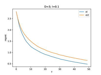
In this example, EI performs slightly better than EI2. To gain a more quantitative understanding, it is instructive to look at how many evaluations $T$ are required to attain a given regret $R=r(l,D,T)$ :

T=t(R,l,D).

(58)

We can then compare the required number of steps for EI and EI2:

\frac{t_{ei}(R,l,D)}{t_{ei2}(R,l,D)},

(59)

which we report in Table 1.

Table 1: Fraction

\frac{t_{ei}(R,l,D)}{t_{ei2}(R,l,D)}

for continuous domains. NaN entries correspond to the case where the given regret was not attained after

T=50

evaluations.

		2.5	2.0	1.5	1.0	0.5
D	l
1	0.003	1.00	1.00	0.87	0.84	NaN
	0.010	1.00	1.00	0.80	0.80	0.74
	0.030	1.00	1.00	1.00	1.00	0.78
	0.100	1.00	1.00	1.00	1.00	0.75
	0.300	1.00	1.00	1.00	1.00	1.00
2	0.003	1.00	1.00	1.00	1.00	NaN
	0.010	1.00	0.86	1.00	NaN	NaN
	0.030	0.67	1.00	0.91	0.71	NaN
	0.100	1.00	1.00	0.80	0.78	0.75
	0.300	1.00	1.00	1.00	1.00	0.83
3	0.003	1.00	1.00	1.00	1.00	NaN
	0.010	1.00	1.00	1.00	NaN	NaN
	0.030	1.00	1.00	1.06	NaN	NaN
	0.100	1.00	1.00	0.73	0.69	NaN
	0.300	1.00	1.00	0.75	0.86	0.73
4	0.003	1.00	1.00	1.00	NaN	NaN
	0.010	1.00	1.00	1.00	NaN	NaN
	0.030	1.00	1.00	1.00	NaN	NaN
	0.100	1.00	1.00	0.84	NaN	NaN
	0.300	1.00	0.75	0.86	0.71	0.70

In one entry EI2 appears to perform slightly better, we have $t_{ei2}=1.06t_{ei}$ . This is may be due to the variance of the empirical estimation. In all other entries, we have $0.5t_{ei2}\leq t_{ei}\leq t_{ei2}$ , which means that EI always reaches the given expected regret $R$ faster than EI2, but not more than twice as fast. This is what we intuitively expected: EI should do better than EI2, because it does not waste evaluations on minimization, but not much better, since in expectation every second evaluation of EI2 is a maximization. Note that the entries which are $1$ , i.e. both algorithms perform equally well, correspond to i) particularly simple settings (large $l$ , low $D$ ) where both algorithms find good values in just a handful of evaluations or ii) particularly hard settings where there is no essentially no correlation between different points in the discretized domain.

For UCB and UCB2 (where we used a fixed confidence level) we obtain similar results, see Table 2.

Table 2: Fraction

\frac{t_{ucb}(R,l,D)}{t_{ucb2}(R,l,D)}

for continuous domains. NaN entries correspond to the case where the given regret was not attained after

T=50

evaluations.

		2.5	2.0	1.5	1.0	0.5
D	l
1	0.003	1.00	1.00	0.89	0.86	NaN
	0.010	1.00	1.00	0.80	0.90	0.81
	0.030	1.00	1.00	1.00	1.00	0.90
	0.100	1.00	1.00	1.00	1.00	1.00
	0.300	1.00	1.00	1.00	1.00	1.00
2	0.003	1.00	1.00	1.00	1.00	NaN
	0.010	1.00	0.86	1.00	NaN	NaN
	0.030	0.67	0.83	0.83	0.77	NaN
	0.100	1.00	1.00	0.80	0.73	0.78
	0.300	1.00	1.00	1.00	1.00	0.83
3	0.003	1.00	1.00	1.00	1.00	NaN
	0.010	1.00	1.00	1.00	NaN	NaN
	0.030	1.00	1.00	1.00	NaN	NaN
	0.100	1.00	0.83	0.75	0.76	NaN
	0.300	1.00	1.00	0.75	1.00	0.71
4	0.003	1.00	1.00	1.00	NaN	NaN
	0.010	1.00	1.00	1.00	NaN	NaN
	0.030	1.00	1.00	1.00	NaN	NaN
	0.100	1.00	0.86	0.83	NaN	NaN
	0.300	1.00	0.75	0.87	0.75	0.66

F.2 Band Covariance Matrices

Next, we compare EI/UCB with EI2/UCB2 in the discrete setting with $N=100$ . We use band covariance matrices, where the diagonal elements are equal to $1$ and there are a number of nonzero elements to the right and the left of the diagonal. We vary width of this band and the value the off-diagonal elements take, we report the results in Table 3 for EI vs EI2 and in Table 4 for UCB vs UCB2. Similarly to the case of continuous domains, we see that $0.5t_{ei2}\leq t_{ei}\leq t_{ei2}$ (and the equivalent for UCB).

Table 3: Fraction

\frac{t_{ei}(\text{band\_size, band\_corr})}{t_{ei2}(\text{band\_size, band\_corr})}

for finite band covariance matrices. The covariance matries are identity matrices with band_size many elements with value band_corr added to each side of the diagonal. NaN entries correspond to the case where the given regret was not attained after

T=20

evaluations.

		2.00	1.55	1.10	0.65	0.20
band_size	band_corr
0	0.00	1.0	1.00	1.00	NaN	NaN
2	-0.20	1.0	0.75	0.86	0.82	NaN
3	0.20	1.0	1.00	0.87	0.89	NaN
5	-0.10	1.0	1.00	1.00	0.94	NaN
	0.20	1.0	1.00	1.00	0.88	NaN
10	0.10	1.0	1.00	1.00	0.94	NaN
40	0.05	1.0	1.00	0.87	0.94	NaN

Table 4: Fraction

\frac{t_{ucb}(\text{band\_size, band\_corr})}{t_{ucb2}(\text{band\_size, band\_corr})}

T=20

evaluations.

		2.00	1.55	1.10	0.65	0.20
band_size	band_corr
0	0.00	1.0	1.0	1.00	NaN	NaN
2	-0.20	1.0	1.0	0.86	0.87	NaN
3	0.20	1.0	1.0	0.87	0.89	NaN
5	-0.10	1.0	1.0	1.00	0.88	NaN
	0.20	1.0	1.0	1.00	0.88	NaN
10	0.10	1.0	1.0	1.00	0.83	NaN
40	0.05	1.0	1.0	1.00	1.00	NaN

F.3 Randomly-Sampled Covariance Matrices

Finally, we sample covariances (of size $N=200$ ) randomly from an inverse Wishart distribution (with $400$ degrees of freedom and identity scale matrix). We report the results in Table 5 for EI vs EI2 and in Table 6 for UCB vs UCB2. As in the previous experiments, we see that $0.5t_{ei2}\leq t_{ei}\leq t_{ei2}$ (and the equivalent for UCB).

Table 5: Fraction

\frac{t_{ei}(\text{wishart\_seed})}{t_{ei2}(\text{wishart\_seed})}

for covariance matrices drawn from a Wishart distribution. NaN entries correspond to the case where the given regret was not attained after

T=30

evaluations.

	0.20	0.15	0.10	0.05	0.00
wishart_seed
1	1.0	0.67	0.83	0.78	NaN
2	1.0	1.00	0.83	0.87	NaN
3	1.0	1.00	0.83	0.83	NaN
4	1.0	1.00	1.00	0.82	NaN
5	1.0	1.00	1.00	0.82	NaN

Table 6: Fraction

\frac{t_{ucb}(\text{wishart\_seed})}{t_{ucb2}(\text{wishart\_seed})}

for covariance matrices drawn from a Wishart distribution. NaN entries correspond to the case where the given regret was not attained after

T=30

evaluations.

	0.20	0.15	0.10	0.05	0.00
wishart_seed
1	1.0	1.0	0.83	0.82	NaN
2	1.0	1.0	0.83	0.87	NaN
3	1.0	1.0	0.83	0.88	NaN
4	1.0	1.0	1.00	0.87	NaN
5	1.0	1.0	1.00	0.81	NaN

Appendix G Proof of Theorem 1

In this section we prove Theorem 1. As we have seen in the previous section, our problem is not adaptively submodular. Nevertheless, the following proof is heavily inspired by the proof in Golovin and Krause [2011]. We derive a less strict condition than adaptive submodularity which is applicable to our problem and implies that we converge exponentially to the optimum $\cdot\beta$ :

Lemma 3.

For any problem of the type defined in Section 2.1, we have for any $\alpha,\beta>0$

$\displaystyle\beta\mathbb{E}\left[\hat{\check{F}}\right]-\mathbb{E}\left[\hat{\check{Y}}_{t}\right]$	$\displaystyle\leq\alpha\left(\mathbb{E}\left[\hat{\check{Y}}_{t+1}\right]-\mathbb{E}\left[\hat{\check{Y}}_{t}\right]\right)\quad\forall t\in\{1:T-1\}$	(60)
	$\displaystyle\Downarrow$
$\displaystyle(1-e^{-\frac{T-1}{\alpha}})\beta\mathbb{E}\left[\hat{\check{F}}\right]$	$\displaystyle\leq\mathbb{E}\left[\hat{\check{Y}}_{T}\right].$	(61)

i.e. the first inequality implies the second inequality.

Proof.

The proof is closely related to the adaptive submodularity proof by Golovin and Krause [2011]. Defining $\delta_{t}:=\beta\mathbb{E}\left[\hat{\check{F}}\right]-\mathbb{E}\left[\hat{\check{Y}}_{t}\right]\forall t\in\{1:T\}$ , we can rewrite the first inequality as

	$\displaystyle\delta_{t}$	$\displaystyle\leq\alpha(\delta_{t}-\delta_{t+1})\quad\forall t\in\{1:T-1\}$
	$\displaystyle\delta_{t+1}$	$\displaystyle\leq(1-\frac{1}{\alpha})\delta_{t}\quad\forall t\in\{1:T-1\}$

Since the function $e^{x}$ is convex, we have $e^{x}\geq 1+x\quad\forall x$ . Using this fact, we obtain the inequality

	$\displaystyle\delta_{t+1}$	$\displaystyle\leq e^{-\frac{1}{\alpha}}\delta_{t}\quad\forall t\in\{1:T-1\}$
	$\displaystyle\delta_{T}$	$\displaystyle\leq e^{-\frac{T-1}{\alpha}}\delta_{1}$

Now we can substitute $\delta_{T}=\beta\mathbb{E}\left[\hat{\check{F}}\right]-\mathbb{E}\left[\hat{\check{Y}}_{T}\right]$ and $\delta_{1}=\beta\mathbb{E}\left[\hat{\check{F}}\right]-\mathbb{E}\left[\hat{\check{Y}}_{1}\right]=\beta\mathbb{E}\left[\hat{\check{F}}\right]$ (since $\hat{\check{Y}}_{1}=0)$ :

	$\displaystyle\beta\mathbb{E}\left[\hat{\check{F}}\right]-\mathbb{E}\left[\hat{\check{Y}}_{T}\right]$	$\displaystyle\leq e^{-\frac{T-1}{\alpha}}\beta\mathbb{E}\left[\hat{\check{F}}\right]$
	$\displaystyle(1-e^{-\frac{T-1}{\alpha}})\beta\mathbb{E}\left[\hat{\check{F}}\right]$	$\displaystyle\leq\mathbb{E}\left[\hat{\check{Y}}_{T}\right].$

∎

Hence, if for some $\alpha,\beta>0$ we can show that 60 holds, Lemma 3 yields a lower bound on the expected utility.

G.1 Specialization for the Extremization Problem

Lemma 4.

For any problem of the type defined in Section 2.1 we have for any $\alpha,\beta>0$

$\displaystyle\mathbb{E}\left[\beta\hat{\check{F}}-\hat{\check{Y}}_{t}\|m_{t},c_{t},\hat{y}_{t},\check{y}_{t}\right]$	$\displaystyle\leq\alpha\mathbb{E}\left[\hat{\check{Y}}_{t+1}-\hat{\check{Y}}_{t}\|m_{t},c_{t},\hat{y}_{t},\check{y}_{t}\right]$	(62)
	$\displaystyle\quad\quad\quad\quad\forall t\in\{1:T-1\},m_{t}\in\mathbb{R}^{N},c_{t}\in\mathbb{S}_{+}^{N},\hat{y}_{t}\geq\check{y}_{t}\in\mathbb{R}$
	$\displaystyle\Downarrow$
$\displaystyle(1-e^{-\frac{T-1}{\alpha}})\beta\mathbb{E}\left[\hat{\check{F}}\right]$	$\displaystyle\leq\mathbb{E}\left[\hat{\check{Y}}\right].$	(63)

Proof.

It is easy to see that the implication

$\displaystyle\mathbb{E}\left[\beta\hat{\check{F}}-\hat{\check{Y}}_{t}\|m_{t},c_{t},\hat{y}_{t},\check{y}_{t}\right]$	$\displaystyle\leq\alpha\mathbb{E}\left[\hat{\check{Y}}_{t+1}-\hat{\check{Y}}_{t}\|m_{t},c_{t},\hat{y}_{t},\check{y}_{t}\right]$	(64)
	$\displaystyle\quad\quad\quad\quad\forall t\in[T-1],m_{t}\in\mathbb{R}^{N},c_{t}\in\mathbb{S}_{+}^{N},\hat{y}_{t}\geq\check{y}_{t}\in\mathbb{R}$
	$\displaystyle\Downarrow$
$\displaystyle\mathbb{E}\left[\beta\hat{\check{F}}-\hat{\check{Y}}_{t}\right]$	$\displaystyle\leq\alpha\mathbb{E}\left[\hat{\check{Y}}_{t+1}-\hat{\check{Y}}_{t}\right]\quad\forall t\in\{1:T-1\}.$	(65)

holds, since taking the expectation with respect to $M_{t},C_{t},\hat{Y}_{t},\check{Y}_{t}$ on both sides of the first line yields the second line. Since 65 is identical to Lemma 3, the desired implication follows from these two implications. ∎

To prove that 62 holds, we will derive a lower bound for the right-hand side and an upper bound for the left-hand side.

G.2 Lower Bound for the Right-Hand Side

Lemma 5.

For any instance $(N,T,\mu,\Sigma)$ of the problem defined in Section 2.1, if we follow either the EI2 (Definition 2) or the UCB2 (Definition 3) strategy, we have

	$\displaystyle\mathbb{E}$	$\displaystyle\left[\hat{\check{Y}}_{t+1}-\hat{\check{Y}}_{t}\|m_{t},c_{t},\hat{y}_{t},\check{y}_{t}\right]$		(66)
		$\displaystyle\geq\max\left\{\operatorname{ei}\left(\hat{y}_{t}\bigg{\|}m_{t}^{n_{ucb}},\sqrt{c_{t}^{n_{ucb}n_{ucb}}}\right),\operatorname{ei}\left(-\check{y}_{t}\bigg{\|}-m_{t}^{n_{ucb}},\sqrt{c_{t}^{n_{ucb}n_{ucb}}}\right)\right\}$

with $\operatorname*{ei}$ as defined in Definition 1 and

n_{ucb}:=\operatorname*{argmax}_{n\in[N]}\max\left\{-\hat{y}_{t}+m_{t}^{n}+\sqrt{c_{t}^{nn}2\log N},\check{y}_{t}-m_{t}^{n}+\sqrt{c_{t}^{nn}2\log N}\right\}

(67)

for any $t\in\{1:T-1\},m_{t}\in\mathbb{R}^{N},c_{t}\in\mathbb{S}_{+}^{N},\hat{y}_{t}\geq\check{y}_{t}\in\mathbb{R}$ .

Proof.

Developing the expectation on the left hand side of 62 we have

$\displaystyle\mathbb{E}$	$\displaystyle\left[\hat{\check{Y}}_{t+1}-\hat{\check{Y}}_{t}\|m_{t},c_{t},\hat{y}_{t},\check{y}_{t}\right]$	(68)
	$\displaystyle=\mathbb{E}\left[\max\left\{F_{A_{t+1}}-\hat{y}_{t},0\right\}+\max\left\{-F_{A_{t+1}}+\check{y}_{t},0\right\}\bigg{\|}m_{t},c_{t},\hat{y}_{t},\check{y}_{t}\right]$	(69)
	$\displaystyle=\mathbb{E}\left[\operatorname{ei}\left(\hat{y}_{t}\bigg{\|}m_{t}^{A_{t+1}},\sqrt{c_{t}^{A_{t+1}A_{t+1}}}\right)+\operatorname{ei}\left(-\check{y}_{t}\bigg{\|}-m_{t}^{A_{t+1}},\sqrt{c_{t}^{A_{t+1}A_{t+1}}}\right)\bigg{\|}m_{t},c_{t},\hat{y}_{t},\check{y}_{t}\right]$	(70)
	$\displaystyle\geq\mathbb{E}\left[\max\left\{\operatorname{ei}\left(\hat{y}_{t}\bigg{\|}m_{t}^{A_{t+1}},\sqrt{c_{t}^{A_{t+1}A_{t+1}}}\right),\operatorname{ei}\left(-\check{y}_{t}\bigg{\|}-m_{t}^{A_{t+1}},\sqrt{c_{t}^{A_{t+1}A_{t+1}}}\right)\right\}\bigg{\|}m_{t},c_{t},\hat{y}_{t},\check{y}_{t}\right]$	(71)

where we have used Definition 1, and the inequality follows from the fact that the expected improvement ( $\operatorname*{ei}$ ) is always $\geq 0$ . The action $A_{t+1}$ is a function of $M_{t},C_{t},\hat{Y}_{t},\check{Y}_{t}$ . If we follow the EI2 strategy (Definition 2), we have

\displaystyle=\max_{n\in[N]}\max\left\{\operatorname*{ei}\left(\hat{y}_{t}|m_{t}^{n},\sqrt{c_{t}^{nn}}\right),\operatorname*{ei}\left(-\check{y}_{t}|-m_{t}^{n},\sqrt{c_{t}^{nn}}\right)\right\}

(72)

and if we follow the UCB2 (Definition 3) strategy, we have

\lx@cref{creftypecap~refnum}{bla}=\max\left\{\operatorname*{ei}\left(\hat{y}_{t}\bigg{|}m_{t}^{n_{ucb}},\sqrt{c_{t}^{n_{ucb}n_{ucb}}}\right),\operatorname*{ei}\left(-\check{y}_{t}\bigg{|}-m_{t}^{n_{ucb}},\sqrt{c_{t}^{n_{ucb}n_{ucb}}}\right)\right\}.

(73)

Clearly we have $\lx@cref{creftypecap~refnum}{eq:rhs_intermediate_ei}\geq\lx@cref{creftypecap~refnum}{eq:rhs_intermediate_ucb}$ , hence for both strategies it holds that $\lx@cref{creftypecap~refnum}{bla}\geq\lx@cref{creftypecap~refnum}{eq:rhs_intermediate_ucb}$ which concludes the proof.

∎

G.3 Upper Bound for the Left-Hand Side

In analogy with Definition 1, we define

Definition 8 (Multivariate Expected Improvement).

For a family of jointly Gaussian distributed RVs $(F_{n})_{n\in[N]}$ with mean $m\in\mathbb{R}^{N}$ and covariance $c\in\mathbb{S}_{+}^{N}$ and a threshold $\tau\in\mathbb{R}$ , we define the multivariate expected improvement as

	$\displaystyle\operatorname*{mei}(\tau\|m,c):$	$\displaystyle=\mathbb{E}\left[\max\left\{\max_{n\in[N]}F_{n}-\tau,0\right\}\right]$		(74)
		$\displaystyle=\int_{\mathbb{R}^{N}}\max\left\{\max_{n\in[N]}f_{n}-\tau,0\right\}\mathcal{N}(f\|m,c)df.$		(75)

Lemma 6.

For any instance $(N,T,\mu,\Sigma)$ of the problem defined in Section 2.1, if we follow either the EI2 (Definition 2) or the UCB2 (Definition 3) strategy, we have for any $0<\beta\leq 1$

	$\displaystyle\mathbb{E}$	$\displaystyle\left[\beta\hat{\check{F}}-\hat{\check{Y}}_{t}\|m_{t},c_{t},\hat{y}_{t},\check{y}_{t}\right]$		(76)
		$\displaystyle\leq\beta 2\max\left\{\operatorname{mei}(0\|m_{t}-\hat{y}_{t},c_{t}),\operatorname{mei}(0\|\check{y}_{t}-m_{t},c_{t})\right\}+(1-\beta)(-\hat{y}_{t}+\check{y}_{t})$

for any $t\in\{1:T-1\},m_{t}\in\mathbb{R}^{N},c_{t}\in\mathbb{S}_{+}^{N},\hat{y}_{t}\geq\check{y}_{t}\in\mathbb{R}$ .

Proof.

We have

$\displaystyle\mathbb{E}$	$\displaystyle\left[\beta\hat{\check{F}}-\hat{\check{Y}}_{t}\|m_{t},c_{t},\hat{y}_{t},\check{y}_{t}\right]$	(77)
	$\displaystyle=\beta\mathbb{E}\left[\hat{F}-\check{F}-\hat{y}_{t}+\check{y}_{t}\|m_{t},c_{t}\right]+(1-\beta)(-\hat{y}_{t}+\check{y}_{t})$	(78)
	$\displaystyle=\beta\mathbb{E}\left[\hat{F}-\hat{y}_{t}\|m_{t},c_{t}\right]+\beta\mathbb{E}\left[-\check{F}+\check{y}_{t}\|m_{t},c_{t}\right]+(1-\beta)(-\hat{y}_{t}+\check{y}_{t})$	(79)
	$\displaystyle\leq\beta\mathbb{E}\left[\max\{\hat{F}-\hat{y}_{t},0\}\|m_{t},c_{t}\right]+\beta\mathbb{E}\left[\max\{-\check{F}+\check{y}_{t},0\}\|m_{t},c_{t}\right]+(1-\beta)(-\hat{y}_{t}+\check{y}_{t})$	(80)
	$\displaystyle=\beta\left(\operatorname{mei}(0\|m_{t}-\hat{y}_{t},c_{t})+\operatorname{mei}(0\|\check{y}_{t}-m_{t},c_{t})\right)+(1-\beta)(-\hat{y}_{t}+\check{y}_{t})$	(81)
	$\displaystyle\leq\beta 2\max\left\{\operatorname{mei}(0\|m_{t}-\hat{y}_{t},c_{t}),\operatorname{mei}(0\|\check{y}_{t}-m_{t},c_{t})\right\}+(1-\beta)(-\hat{y}_{t}+\check{y}_{t})$	(82)

where by $m_{t}-\hat{y}_{t}$ we mean that the scalar $\hat{y}_{t}$ is subtracted from each element of the vector $m_{t}$ .

∎

G.4 Upper Bound on the Regret

Theorem 4.

For any instance $(N,T,\mu,\Sigma)$ of the problem defined in Section 2.1, if we follow either the EI2 (Definition 2) or the UCB2 (Definition 3) strategy, we have for any $\alpha>0$ and any $0<\beta\leq 1-\frac{1}{\sqrt{2\pi}\left(2\log N\right)^{3/2}}$

$\displaystyle\max_{x}\left(2\frac{\beta\left(\sqrt{2\log N}+\frac{1}{2\log N\sqrt{2\pi}}\right)-x}{\operatorname*{ei}\left(x\right)}\right)$	$\displaystyle\leq\alpha$	(83)
	$\displaystyle\Downarrow$
$\displaystyle(1-e^{-\frac{T-1}{\alpha}})\beta\mathbb{E}\left[\hat{\check{F}}\right]$	$\displaystyle\leq\mathbb{E}\left[\hat{\check{Y}}\right]$	(84)

i.e. the first line implies the second.

Proof.

According to Lemma 4, we have


	$\displaystyle\Uparrow$
	$\displaystyle\frac{\mathbb{E}\left[\beta\hat{\check{F}}-\hat{\check{Y}}_{t}\|m_{t},c_{t},\hat{y}_{t},\check{y}_{t}\right]}{\mathbb{E}\left[\hat{\check{Y}}_{t+1}-\hat{\check{Y}}_{t}\|m_{t},c_{t},\hat{y}_{t},\check{y}_{t}\right]}\leq\alpha$
	$\displaystyle\quad\quad\forall t\in\{1:T-1\},m_{t}\in\mathbb{R}^{N},c_{t}\in\mathbb{S}_{+}^{N},\hat{y}_{t}\geq\check{y}_{t}\in\mathbb{R}.$		(85)

In the following, we will find a simpler expression which implies 85 and therefore 84. Then we will simplify the new expression further, until we finally arrive at 83 through an unbroken chain of implications.

Using the lower bound from Lemma 5 and the upper bound from Lemma 6 we can write


	$\displaystyle\Uparrow$
	$\displaystyle\frac{\beta 2\max\left\{\operatorname{mei}(0\|m-\hat{y},c),\operatorname{mei}(0\|\check{y}-m,c)\right\}+(1-\beta)(-\hat{y}+\check{y})}{\max\left\{\operatorname{ei}\left(\hat{y}\bigg{\|}m^{n_{ucb}},\sqrt{c^{n_{ucb}n_{ucb}}}\right),\operatorname{ei}\left(-\check{y}\bigg{\|}-m^{n_{ucb}},\sqrt{c^{n_{ucb}n_{ucb}}}\right)\right\}}\leq\alpha$
	$\displaystyle\quad\quad\forall m\in\mathbb{R}^{N},c\in\mathbb{S}_{+}^{N},\hat{y}\geq\check{y}\in\mathbb{R},$		(86)
	$\displaystyle\quad\quad\quad\quad n_{ucb}=\operatorname*{argmax}_{n\in[N]}\max\left\{-\hat{y}+m^{n}+\sqrt{c^{nn}2\log N},\check{y}-m^{n}+\sqrt{c^{nn}2\log N}\right\}$

where we have dropped the time indices, since they are irrelevant here. It is easy to see that all terms in 86 are invariant to a common shift in $m,\hat{y}$ and $\check{y}$ . Hence, we can impose a constraint on these variables, without changing the condition. We choose the constraint $\hat{y}=-\check{y}$ to simplify the expression


	$\displaystyle\Updownarrow$
	$\displaystyle 2\frac{\beta\max\left\{\operatorname{mei}(0\|m-\hat{y},c),\operatorname{mei}(0\|-\hat{y}-m,c)\right\}-(1-\beta)\hat{y}}{\max\left\{\operatorname{ei}\left(\hat{y}\bigg{\|}m^{n_{ucb}},\sqrt{c^{n_{ucb}n_{ucb}}}\right),\operatorname{ei}\left(\hat{y}\bigg{\|}-m^{n_{ucb}},\sqrt{c^{n_{ucb}n_{ucb}}}\right)\right\}}\leq\alpha$
	$\displaystyle\quad\quad\forall m\in\mathbb{R}^{N},c\in\mathbb{S}_{+}^{N},\hat{y}\in\mathbb{R}_{\geq 0},$		(87)
	$\displaystyle\quad\quad\quad\quad n_{ucb}=\operatorname*{argmax}_{n\in[N]}\max\left\{-\hat{y}+m^{n}+\sqrt{c^{nn}2\log N},-\hat{y}-m^{n}+\sqrt{c^{nn}2\log N}\right\}.$

Clearly, the denominator is invariant with respect to any sign flips in the elements of $m$ . The numerator is maximized if all elements of $m$ have the same sign, no matter if positive or negative. Hence, we can restrict the above conditions to $m$ with positive entries, which means in all maximum operators the left term is active


	$\displaystyle\Updownarrow$
	$\displaystyle 2\frac{\beta\operatorname{mei}(0\|m-\hat{y},c)-(1-\beta)\hat{y}}{\operatorname{ei}\left(\hat{y}\bigg{\|}m^{n_{ucb}},\sqrt{c^{n_{ucb}n_{ucb}}}\right)}\leq\alpha$
	$\displaystyle\quad\quad\forall m\in\mathbb{R}_{\geq 0}^{N},c\in\mathbb{S}_{+}^{N},\hat{y}\in\mathbb{R}_{\geq 0},n_{ucb}=\operatorname*{argmax}_{n\in[N]}\left(m^{n}+\sqrt{c^{nn}2\log N}\right).$		(88)

Inserting the bound from Lemma 12 we have


	$\displaystyle\Uparrow$
	$\displaystyle 2\frac{\beta\left(\max\left\{\max_{n\in[N]}(m^{n}-\hat{y}+\sqrt{c^{nn}2\log N}),0\right\}+\frac{\max_{n\in[N]}\sqrt{c^{nn}}}{2\sqrt{2\pi}\log\left(N\right)}\right)-(1-\beta)\hat{y}}{\operatorname*{ei}\left(\hat{y}\bigg{\|}m^{n_{ucb}},\sqrt{c^{n_{ucb}n_{ucb}}}\right)}\leq\alpha$
	$\displaystyle\quad\quad\forall m\in\mathbb{R}_{\geq 0}^{N},c\in\mathbb{S}_{+}^{N},\leq\alpha,\hat{y}\in\mathbb{R}_{\geq 0},n_{ucb}=\operatorname*{argmax}_{n\in[N]}\left(m^{n}+\sqrt{c^{nn}2\log N}\right)$		(89)
	$\displaystyle\Updownarrow$
	$\displaystyle 2\frac{\beta\left(\max\left\{m^{n_{ucb}}-\hat{y}+\sqrt{c^{n_{ucb}n_{ucb}}2\log N},0\right\}+\frac{\max_{n\in[N]}\sqrt{c^{nn}}}{2\sqrt{2\pi}\log\left(N\right)}\right)-(1-\beta)\hat{y}}{\operatorname*{ei}\left(\hat{y}\bigg{\|}m^{n_{ucb}},\sqrt{c^{n_{ucb}n_{ucb}}}\right)}\leq\alpha$
	$\displaystyle\quad\quad\forall m\in\mathbb{R}_{\geq 0}^{N},c\in\mathbb{S}_{+}^{N},\leq\alpha,\hat{y}\in\mathbb{R}_{\geq 0},n_{ucb}=\operatorname*{argmax}_{n\in[N]}\left(m^{n}+\sqrt{c^{nn}2\log N}\right).$		(90)

It holds for any $n\in[N]$ that $m^{n}\geq 0$ and

m^{n_{ucb}}+\sqrt{c^{n_{ucb}n_{ucb}}}\sqrt{2\log N}\geq m^{n}+\sqrt{c^{nn}2\log N},

from which it follows that

\displaystyle\frac{m^{n_{ucb}}}{\sqrt{2\log N}}+\sqrt{c^{n_{ucb}n_{ucb}}}

\displaystyle\geq\sqrt{c^{nn}}.

(91)

Using this fact we can write


	$\displaystyle\Uparrow$
	$\displaystyle 2\frac{\beta\left(\max\{m^{n_{ucb}}-\hat{y}+\sqrt{c^{n_{ucb}n_{ucb}}}\sqrt{2\log N},0\}+\frac{\sqrt{c^{n_{ucb}n_{ucb}}}}{2\log N\sqrt{2\pi}}+\frac{m^{n_{ucb}}}{\sqrt{2\pi}\left(2\log N\right)^{3/2}}\right)-(1-\beta)\hat{y}}{\operatorname*{ei}\left(\hat{y}\bigg{\|}m^{n_{ucb}},\sqrt{c^{n_{ucb}n_{ucb}}}\right)}\leq\alpha$
	$\displaystyle\quad\quad\forall m\in\mathbb{R}_{\geq 0}^{N},c\in\mathbb{S}_{+}^{N},\leq\alpha,\hat{y}\in\mathbb{R}_{\geq 0},n_{ucb}=\operatorname*{argmax}_{n\in[N]}\left(m^{n}+\sqrt{c^{nn}2\log N}\right).$		(92)

For any $\beta\leq 1-\frac{1}{1+\sqrt{2\pi}\left(2\log N\right)^{3/2}}\leq 1-\frac{1}{\sqrt{2\pi}\left(2\log N\right)^{3/2}}$ we have


	$\displaystyle\Uparrow$
	$\displaystyle 2\frac{\beta\left(\max\{m^{n_{ucb}}-\hat{y}+\sqrt{c^{n_{ucb}n_{ucb}}}\sqrt{2\log N},0\}+\frac{\sqrt{c^{n_{ucb}n_{ucb}}}}{2\log N\sqrt{2\pi}}\right)-(1-\beta)(\hat{y}-m^{n_{ucb}})}{\operatorname*{ei}\left(\hat{y}\bigg{\|}m^{n_{ucb}},\sqrt{c^{n_{ucb}n_{ucb}}}\right)}\leq\alpha$
	$\displaystyle\quad\quad\forall m\in\mathbb{R}_{\geq 0}^{N},c\in\mathbb{S}_{+}^{N},\leq\alpha,\hat{y}\in\mathbb{R}_{\geq 0},n_{ucb}=\operatorname*{argmax}_{n\in[N]}\left(m^{n}+\sqrt{c^{nn}2\log N}\right).$		(93)

According to Definition 1, we have

\operatorname*{ei}\left(\hat{y}\bigg{|}\mu,\sqrt{c^{n_{ucb}n_{ucb}}}\right)=\sqrt{c^{n_{ucb}n_{ucb}}}\operatorname*{ei}\left(\frac{\hat{y}-m^{n_{ucb}}}{\sqrt{c^{n_{ucb}n_{ucb}}}}\right).

Using this fact, we obtain


	$\displaystyle\Updownarrow$
	$\displaystyle 2\frac{\beta\left(\max\left\{\frac{m^{n_{ucb}}-\hat{y}}{\sqrt{c^{n_{ucb}n_{ucb}}}}+\sqrt{2\log N},0\right\}+\frac{1}{2\log N\sqrt{2\pi}}\right)-(1-\beta)\frac{\hat{y}-m^{n_{ucb}}}{\sqrt{c^{n_{ucb}n_{ucb}}}}}{\operatorname*{ei}\left(\frac{\hat{y}-m^{n_{ucb}}}{\sqrt{c^{n_{ucb}n_{ucb}}}}\right)}\leq\alpha$
	$\displaystyle\quad\quad\forall m\in\mathbb{R}_{\geq 0}^{N},c\in\mathbb{S}_{+}^{N},\leq\alpha,\hat{y}\in\mathbb{R}_{\geq 0},n_{ucb}=\operatorname*{argmax}_{n\in[N]}\left(m^{n}+\sqrt{c^{nn}2\log N}\right).$		(94)

Defining $x:=\frac{\hat{y}-m^{n_{ucb}}}{\sqrt{c^{n_{ucb}n_{ucb}}}}$ we can simplify this condition as


	$\displaystyle\Updownarrow$
	$\displaystyle 2\frac{\beta\left(\max\left\{\sqrt{2\log N}-x,0\right\}+\frac{1}{2\log N\sqrt{2\pi}}\right)-(1-\beta)x}{\operatorname*{ei}\left(x\right)}\leq\alpha\quad\quad\forall x\in\mathbb{R}.$		(95)

For any $x\geq\sqrt{2\log N}$ the numerator of the left hand side is negative

$\displaystyle\beta\left(\frac{1}{2\log N\sqrt{2\pi}}\right)-(1-\beta)x$	$\displaystyle\leq\beta\left(\frac{1}{2\log N\sqrt{2\pi}}\right)-(1-\beta)\sqrt{2\log N}$	(96)
	$\displaystyle\leq(1-\frac{1}{\sqrt{2\pi}\left(2\log N\right)^{3/2}})\left(\frac{1}{2\log N\sqrt{2\pi}}\right)-\frac{1}{\sqrt{2\pi}\left(2\log N\right)}$	(97)
	$\displaystyle=-\frac{1}{2\log N\sqrt{2\pi}}\left(\frac{1}{2\log N\sqrt{2\pi}}\right)$	(98)
	$\displaystyle\leq 0$	(99)

and since $\alpha$ and the denominator are both positive, 95 is satisfied. Hence, we only need to consider the case where $x\leq\sqrt{2\log N}$ and can therefore write


	$\displaystyle\Updownarrow$
	$\displaystyle 2\frac{\beta\left(\sqrt{2\log N}+\frac{1}{2\log N\sqrt{2\pi}}\right)-x}{\operatorname*{ei}\left(x\right)}\leq\alpha\quad\forall x\leq\sqrt{2\log N}.$		(100)

From this chain of implications and Lemma 4 the result of Theorem 4 follows.∎

Finally, using the previous results, we can obtain the desired bound on the regret (Theorem 1), which we restate here for convenience:

See Theorem 1

Proof.

We can rewrite Theorem 4 as

	$\displaystyle\left(1-e^{-\frac{T}{\max_{x}\left(2\frac{\beta\left(\sqrt{2\log N}+\frac{1}{2\log N\sqrt{2\pi}}\right)-x}{\operatorname*{ei}\left(x\right)}\right)}}\right)\beta$	$\displaystyle\leq\frac{\mathbb{E}\left[\hat{\check{Y}}\right]}{\mathbb{E}\left[\hat{\check{F}}\right]}$		(101)
	$\displaystyle\forall N\geq T\geq 500,\mu,\Sigma,$	$\displaystyle 0<\beta\leq 1-\frac{1}{\sqrt{2\pi}\left(2\log N\right)^{3/2}}$

where we have restricted the inequality to $N\geq T\geq 500$ , a condition we need later . What is left to be done is to simplify this bound, such that it becomes interpretable. We can rewrite the above as

	$\displaystyle\left(1-e^{-\frac{T}{\max_{x}\left(2\frac{\beta\left(\frac{1}{\sqrt{2\pi}a^{2}}+a\right)-x}{\operatorname*{ei}\left(x\right)}\right)}}\right)\beta$	$\displaystyle\leq\frac{\mathbb{E}\left[\hat{\check{Y}}\right]}{\mathbb{E}\left[\hat{\check{F}}\right]}$		(102)
	$\displaystyle\forall N\geq T\geq 500,\mu,\Sigma,$	$\displaystyle 0<\beta\leq 1-\frac{1}{\sqrt{2\pi}a^{3}},a=\sqrt{2\log N}.$

Choosing a $\beta$

We choose

\displaystyle\beta

\displaystyle\text{=}\frac{b-\frac{\text{ei}(b)}{\text{ei}^{\prime}(b)}}{\frac{1}{\sqrt{2\pi}a^{2}}+a}

(103)

where $\text{ei}^{\prime}$ is the derivative of ei, and

b=\sqrt{\sqrt{2\log T}^{2}-2\log\left(3\ 2^{-3/2}\sqrt{2\log T}^{3}\right)}.

(104)

Before we can continue, we need to show that this $\beta$ satisfies the condition in 102. First of all, from 104 and the conditions in 102 we can derive some relations which will be useful later on

\displaystyle 2.17\leq b

\displaystyle\leq\sqrt{a^{2}-2\log\left(3\ 2^{-3/2}a^{3}\right)}\leq a.

(105)

It is easy to see that $0<\beta$ holds, it remains to be shown that

\displaystyle\beta

\displaystyle\leq 1-\frac{1}{\sqrt{2\pi}a^{3}}.

(106)

Inserting the definition of $\beta$ 103 and simplifying we have

	$\displaystyle\frac{b-\frac{\text{ei}(b)}{\text{ei}^{\prime}(b)}}{\frac{1}{\sqrt{2\pi}a^{2}}+a}$	$\displaystyle\leq 1-\frac{1}{\sqrt{2\pi}a^{3}}$		(107)
	$\displaystyle b-\frac{\text{ei}(b)}{\text{ei}^{\prime}(b)}$	$\displaystyle\leq a-\frac{1}{2\pi a^{5}}.$		(108)

Using Definition 1 and the lower bound in Lemma 10, we obtain a sufficient condition

\frac{b^{3}}{b^{2}-1}\leq a-\frac{1}{2\pi a^{5}}.

(109)

Since we have $b\leq a$ (see 105) we obtain the sufficient condition

\frac{1}{2\pi b^{5}}+\frac{b^{3}}{b^{2}-1}\leq a.

(110)

From $2.17\leq b$ (see 105) it follows that $2\pi b^{5}\geq b^{2}-1$ , and hence we can further simplify to obtain a sufficient condition

b+\frac{1}{b-1}\leq a.

(111)

Given 105 it is easy to see that both sides are positive, hence we can square each side to obtain

b^{2}+\frac{2b}{b-1}+\frac{1}{(b-1)^{2}}\leq a^{2}.

(112)

Now we will show that this condition is satisfied by 104. We have from 105

	$\displaystyle b$	$\displaystyle\leq\sqrt{a^{2}-2\log\left(3\ 2^{-3/2}a^{3}\right)}$		(113)
	$\displaystyle 2\log\left(3\ 2^{-3/2}a^{3}\right)+b^{2}$	$\displaystyle\leq a^{2}$		(114)

and since $b\leq a$ , we have

2\log\left(3\ 2^{-3/2}b^{3}\right)+b^{2}\leq a^{2}.

(115)

This implies 112, to see this we use the above inequality to bound $a^{2}$ in 112

	$\displaystyle b^{2}+\frac{2b}{b-1}+\frac{1}{(b-1)^{2}}$	$\displaystyle\leq 2\log\left(3\ 2^{-3/2}b^{3}\right)+b^{2}$		(116)
	$\displaystyle\frac{2b}{b-1}+\frac{1}{(b-1)^{2}}$	$\displaystyle\leq 2\log\left(3\ 2^{-3/2}b^{3}\right).$		(117)

It is easy to verify that for any $b\geq 2.17$ , the left-hand side is decreasing and the right-hand side is increasing. Hence, it is sufficient to show that it holds for $b=2.17$ which is easily done by evaluating at that value. This concludes the proof that our choice of $\beta$ 103 satisfies the conditions in 102. We can now insert this value to obtain

	$\displaystyle\left(1-e^{-\frac{T}{\max_{x}\left(2\frac{b-\frac{\text{ei}(b)}{\text{ei}^{\prime}(b)}-x}{\operatorname*{ei}\left(x\right)}\right)}}\right)\frac{b-\frac{\text{ei}(b)}{\text{ei}^{\prime}(b)}}{\frac{1}{\sqrt{2\pi}a^{2}}+a}$	$\displaystyle\leq\frac{\mathbb{E}\left[\hat{\check{Y}}\right]}{\mathbb{E}\left[\hat{\check{F}}\right]}$		(118)
	$\displaystyle\forall N\geq T\geq 500,\bar{\mu},\Sigma,a=\sqrt{2\log N},$	$\displaystyle b=\sqrt{\sqrt{2\log T}^{2}-2\log\left(3\ 2^{-3/2}\sqrt{2\log T}^{3}\right)}$

Optimizing for $x$

Here we show that

\max_{x}\left(2\frac{b-\frac{\text{ei}(b)}{\text{ei}^{\prime}(b)}-x}{\operatorname*{ei}\left(x\right)}\right)\leq-\frac{2}{\text{ei}^{\prime}(b)}.

(119)

We have

	$\displaystyle\max_{x}\left(2\frac{b-\frac{\text{ei}(b)}{\text{ei}^{\prime}(b)}-x}{\operatorname*{ei}\left(x\right)}\right)$	$\displaystyle=\max_{\delta}\left(2\frac{b-\frac{\text{ei}(b)}{\text{ei}^{\prime}(b)}-b-\delta}{\operatorname*{ei}\left(b+\delta\right)}\right)$		(120)
		$\displaystyle=\max_{\delta}\left(2\frac{\text{ei}(b)+\delta\text{ei}^{\prime}(b)}{-\text{ei}^{\prime}(b)\operatorname*{ei}\left(b+\delta\right)}\right).$		(121)

Since the ei function is convex, we have $\text{ei}(b)+\delta\text{ei}^{\prime}(b)\leq\text{ei}(b+\delta)$ . Using this and the fact that the denominator is positive (since ei is always positive and $\operatorname*{ei}^{\prime}$ is always negative), we have

\max_{x}\left(2\frac{b-\frac{\text{ei}(b)}{\text{ei}^{\prime}(b)}-x}{\operatorname*{ei}\left(x\right)}\right)\leq-\frac{2}{\text{ei}^{\prime}(b)}.

(122)

Inserting this result into 118, we obtain

	$\displaystyle\left(1-e^{\frac{T\text{ei}^{\prime}(b)}{2}}\right)\frac{b-\frac{\text{ei}(b)}{\text{ei}^{\prime}(b)}}{\frac{1}{\sqrt{2\pi}a^{2}}+a}$	$\displaystyle\leq\frac{\mathbb{E}\left[\hat{\check{Y}}\right]}{\mathbb{E}\left[\hat{\check{F}}\right]}$		(123)
	$\displaystyle\forall N\geq T\geq 500,\mu,\Sigma,a=\sqrt{2\log N},$	$\displaystyle b=\sqrt{\sqrt{2\log T}^{2}-2\log\left(3\ 2^{-3/2}\sqrt{2\log T}^{3}\right)}.$

Simplifying the bound further

Now, all that is left to do is to simplify this bound a bit further.

Bounding the left factor

First of all, we show that the left factor satisfies

1-e^{\frac{1}{2}T\text{ei}^{\prime}(b)}\geq 1-T^{-\frac{1}{2\sqrt{\pi}}}.

(124)

Using Definition 1 and the lower bound from Lemma 10, we obtain

	$\displaystyle 1-e^{\frac{1}{2}T\text{ei}^{\prime}(b)}$	$\displaystyle\geq 1-e^{-\frac{\left(b^{2}-1\right)e^{-\frac{b^{2}}{2}}T}{2\sqrt{2\pi}b^{3}}}$		(125)
		$\displaystyle\geq 1-e^{-\frac{e^{-\frac{b^{2}}{2}}T}{3\sqrt{2\pi}b}}$		(126)

where the second inequality is easily seen to hold true, since we have $b\geq 2.17$ . Inserting 104, and bounding further we obtain

$\displaystyle 1-e^{-\frac{e^{-\frac{b^{2}}{2}}T}{3\sqrt{2\pi}b}}$	$\displaystyle=1-e^{-\frac{\log^{\frac{3}{2}}(T)}{2\sqrt{\pi}\sqrt{\log(T)-\log\left(3\log^{\frac{3}{2}}(T)\right)}}}$	(127)
	$\displaystyle\geq 1-e^{-\frac{\log^{\frac{3}{2}}(T)}{2\sqrt{\pi}\sqrt{\log(T)}}}$	(128)
	$\displaystyle=1-T^{-\frac{1}{2\sqrt{\pi}}}$	(129)

from which 124 follows.

Bounding the right factor

Now we will show that the right factor from 123 satisfies

\frac{b-\frac{\text{ei}(b)}{\text{ei}^{\prime}(b)}}{\frac{1}{\sqrt{2\pi}a^{2}}+a}\geq\sqrt{\frac{\log(T)-\log\left(3\log^{\frac{3}{2}}(T)\right)}{\log(N)}}.

(130)

Using Definition 1 and the upper bound from Lemma 10, we obtain

\frac{b-\frac{\text{ei}(b)}{\text{ei}^{\prime}(b)}}{\frac{1}{\sqrt{2\pi}a^{2}}+a}\geq\frac{2\sqrt{\pi}a^{2}b^{5}}{\left(2\sqrt{\pi}a^{3}+\sqrt{2}\right)\left(b^{4}-b^{2}+3\right)}.

(131)

Now, to lower bound this further, we show that

\left(2\sqrt{\pi}a^{3}+\sqrt{2}\right)\left(b^{4}-b^{2}+3\right)\leq\left(2\sqrt{\pi}a^{3}\right)b^{4}.

(132)

Equivalently, we can show that

-2\sqrt{\pi}a^{3}b^{2}+6\sqrt{\pi}a^{3}+\sqrt{2}b^{4}-\sqrt{2}b^{2}+3\sqrt{2}\leq 0.

(133)

Since $b\geq 2.17$ , we have $3\sqrt{2}-\sqrt{2}b^{2}\leq 0$ , and hence

-2\sqrt{\pi}a^{3}b^{2}+6\sqrt{\pi}a^{3}+\sqrt{2}b^{4}\leq 0

(134)

is a sufficient condition. The derivative of the left-hand side

	$\displaystyle 4\sqrt{2}b^{2}-4\sqrt{\pi}a^{3}$	$\displaystyle\leq 4\sqrt{2}a^{2}-4\sqrt{\pi}a^{3}$		(135)
		$\displaystyle=(4\sqrt{2}-4\sqrt{\pi}a)a^{2}$		(136)

is always negative (since $a\geq 2.17$ ). Hence, it is sufficient to show that 134 holds for the minimal $b=2.17$ , which can easily be verified to hold true for any $a\geq 2.17$ . Hence, we have shown that 132 holds, and inserting it into 131, we obtain

$\displaystyle\frac{b-\frac{\text{ei}(b)}{\text{ei}^{\prime}(b)}}{\frac{1}{\sqrt{2\pi}a^{2}}+a}$	$\displaystyle\geq\frac{2\sqrt{\pi}a^{2}b^{5}}{\left(2\sqrt{\pi}a^{3}\right)b^{4}}$	(137)
	$\displaystyle=\frac{b}{a}$	(138)
	$\displaystyle=\sqrt{\frac{\log(T)-\log\left(3\log^{\frac{3}{2}}(T)\right)}{\log(N)}}.$	(139)

Final bound

Finally, inserting 124 and 130 into 123, we obtain

\displaystyle\left(1-T^{-\frac{1}{2\sqrt{\pi}}}\right)\sqrt{\frac{\log(T)-\log\left(3\log^{\frac{3}{2}}(T)\right)}{\log(N)}}

\displaystyle\leq\frac{\mathbb{E}\left[\hat{\check{Y}}\right]}{\mathbb{E}\left[\hat{\check{F}}\right]}\quad\forall N\geq T\geq 500,\mu,\Sigma.

(140)

This implies straightforwardly the bound on the regret

\frac{\mathbb{E}\left[\hat{\check{F}}\right]-\mathbb{E}\left[\hat{\check{Y}}\right]}{\mathbb{E}\left[\hat{\check{F}}\right]}\leq 1-\left(1-T^{-\frac{1}{2\sqrt{\pi}}}\right)\sqrt{\frac{\log(T)-\log\left(3\log^{\frac{3}{2}}(T)\right)}{\log(N)}}\quad\forall N\geq T\geq 500,\mu,\Sigma.

(141)

∎

Appendix H Proof of Theorem 3

The proof of Theorem 3 is very similar to the one of Theorem 1 in Appendix G. Here we discuss the parts that are different.

Lemma 7.

For any problem of the type defined in Section 2.1, we have for any $\alpha,\beta>0$

$\displaystyle\beta\mathbb{E}\left[\hat{\check{F}}\right]-\mathbb{E}\left[\hat{Y}_{t}-\check{F}\right]$	$\displaystyle\leq\alpha\left(\mathbb{E}\left[\hat{Y}_{t+1}-\hat{Y}_{t}\right]\right)\quad\forall t\in\{1:T-1\}$	(142)
	$\displaystyle\Downarrow$
$\displaystyle(1-e^{-\frac{T-1}{\alpha}})\beta\mathbb{E}\left[\hat{\check{F}}\right]$	$\displaystyle\leq\mathbb{E}\left[\hat{Y}_{T}-\check{F}\right].$	(143)

i.e. the first inequality implies the second inequality.

Proof.

This result is obtained from Lemma 3 by replacing $\hat{\check{Y}}_{t}$ with $\hat{Y}_{t}-\check{F}$ . It is easy to see that the proof of Lemma 3 goes through with this change.

∎

Hence, if for some $\alpha,\beta>0$ we can show that 142 holds, Lemma 7 yields a lower bound on the expected utility.

Lemma 8.

For any problem of the type defined in Section 2.1 we have for any $\alpha,\beta>0$

$\displaystyle\mathbb{E}\left[\beta\hat{\check{F}}-(\hat{Y}_{t}-\check{F})\|m_{t},c_{t},\hat{y}_{t}\right]$	$\displaystyle\leq\alpha\mathbb{E}\left[\hat{Y}_{t+1}-\hat{Y}_{t}\|m_{t},c_{t},\hat{y}_{t}\right]$	(144)
	$\displaystyle\quad\quad\quad\quad\forall t\in\{1:T-1\},m_{t}\in\mathbb{R}^{N},c_{t}\in\mathbb{S}_{+}^{N},\hat{y}_{t}\in\mathbb{R}$
	$\displaystyle\Downarrow$
$\displaystyle(1-e^{-\frac{T-1}{\alpha}})\beta\mathbb{E}\left[\hat{\check{F}}\right]$	$\displaystyle\leq\mathbb{E}\left[\hat{Y}-\check{F}\right].$	(145)

Proof.

The proof follows the same logic as the one from Lemma 4.

∎

Theorem 5.

For any instance $(N,T,\mu,\Sigma)$ of the problem defined in Section 2.1, if we follow either the EI (Definition 6) or the UCB (Definition 7) strategy, we have for any $\alpha>0$ and any $0<\beta\leq 1-\frac{1}{\sqrt{2\pi}\left(2\log N\right)^{3/2}}$

$\displaystyle\max_{x}\left(2\frac{\beta\left(\sqrt{2\log N}+\frac{1}{2\log N\sqrt{2\pi}}\right)-x}{\operatorname*{ei}\left(x\right)}\right)$	$\displaystyle\leq\alpha$	(146)
	$\displaystyle\Downarrow$
$\displaystyle(1-e^{-\frac{T-1}{\alpha}})\beta\mathbb{E}\left[\hat{\check{F}}\right]$	$\displaystyle\leq\mathbb{E}\left[\hat{Y}-\check{F}\right]$	(147)

i.e. the first line implies the second.

Proof.

According to Lemma 8, we have


	$\displaystyle\Uparrow$
	$\displaystyle\frac{\mathbb{E}\left[\beta\hat{\check{F}}-(\hat{Y}_{t}-\check{F})\|m_{t},c_{t},\hat{y}_{t}\right]}{\mathbb{E}\left[\hat{Y}_{t+1}-\hat{Y}_{t}\|m_{t},c_{t},\hat{y}_{t}\right]}\leq\alpha$
	$\displaystyle\quad\quad\forall t\in\{1:T-1\},m_{t}\in\mathbb{R}^{N},c_{t}\in\mathbb{S}_{+}^{N},\hat{y}_{t}\in\mathbb{R}.$		(148)

Rearranging terms and plugging in the known variable $\hat{y}_{t}$ we have


	$\displaystyle\Updownarrow$		(149)
	$\displaystyle\frac{\beta\mathbb{E}\left[\hat{F}-\hat{y}_{t}\|m_{t},c_{t}\right]-(1-\beta)\mathbb{E}\left[\hat{y}_{t}-\check{F}\|m_{t},c_{t}\right]}{\mathbb{E}\left[\hat{Y}_{t+1}-\hat{y}_{t}\|m_{t},c_{t},\hat{y}_{t}\right]}\leq\alpha$
	$\displaystyle\quad\quad\forall t\in\{1:T-1\},m_{t}\in\mathbb{R}^{N},c_{t}\in\mathbb{S}_{+}^{N},\hat{y}_{t}\in\mathbb{R}.$		(150)

Since the expected minimum function value $\check{F}$ is no larger than the smallest mean $\check{m}_{t}$ , we have


	$\displaystyle\Uparrow$		(151)
	$\displaystyle\frac{\beta\mathbb{E}\left[\hat{F}-\hat{y}_{t}\|m_{t},c_{t}\right]-(1-\beta)(\hat{y}_{t}-\check{m}_{t})}{\mathbb{E}\left[\hat{Y}_{t+1}-\hat{y}_{t}\|m_{t},c_{t},\hat{y}_{t}\right]}\leq\alpha$
	$\displaystyle\quad\quad\forall t\in\{1:T-1\},m_{t}\in\mathbb{R}^{N},c_{t}\in\mathbb{S}_{+}^{N},\hat{y}_{t}\in\mathbb{R}.$		(152)

Since these terms are invariant to a common shift in all variables, we can assume $\check{m}_{t}=0$ without loss of generality, and hence


	$\displaystyle\Updownarrow$		(153)
	$\displaystyle\frac{\beta\mathbb{E}\left[\hat{F}-\hat{y}_{t}\|m_{t},c_{t}\right]-(1-\beta)\hat{y}_{t}}{\mathbb{E}\left[\hat{Y}_{t+1}-\hat{y}_{t}\|m_{t},c_{t},\hat{y}_{t}\right]}\leq\alpha$
	$\displaystyle\quad\quad\forall t\in\{1:T-1\},m_{t}\in\mathbb{R}_{\geq 0}^{N},c_{t}\in\mathbb{S}_{+}^{N},\hat{y}_{t}\in\mathbb{R}_{\geq 0}.$		(154)

We have

$\displaystyle\mathbb{E}\left[\hat{F}-\hat{y}_{t}\|m_{t},c_{t}\right]$	$\displaystyle\leq\mathbb{E}\left[\max\{\hat{F}-\hat{y}_{t},0\}\|m_{t},c_{t}\right]$	(155)
	$\displaystyle=\mathbb{E}\left[\max\{\hat{F},0\}\|m_{t}-\hat{y}_{t},c_{t}\right]$	(156)
	$\displaystyle=\text{mei}(0\|m_{t}-\hat{y}_{t},c_{t})$	(157)

with mei as defined in Definition 8. In addition, we have

	$\displaystyle\mathbb{E}\left[\hat{Y}_{t+1}-\hat{y}_{t}\|m_{t},c_{t},\hat{y}_{t}\right]$	$\displaystyle=\mathbb{E}\left[\max\left\{\hat{Y}_{t+1}-\hat{y}_{t},0\right\}\|m_{t},c_{t},\hat{y}_{t}\right]$		(158)
		$\displaystyle\geq\text{ei}\left(\hat{y}_{t}\|m_{t}^{n_{ucb}},\sqrt{c_{t}^{n_{ucb}n_{ucb}}}\right)$		(159)

with ei as defined in Definition 1. The equality follows from the fact that we know that $\hat{Y}_{t+1}\geq\hat{y}_{t}$ . The inequality follows due to a similar argument as the one in the proof of Lemma 5.

Substituting these terms and dropping the time index, we have


	$\displaystyle\Uparrow$
	$\displaystyle\frac{\beta\operatorname{mei}(0\|m-\hat{y},c)-(1-\beta)\hat{y}}{\operatorname{ei}\left(\hat{y}\bigg{\|}m^{n_{ucb}},\sqrt{c^{n_{ucb}n_{ucb}}}\right)}\leq\alpha$
	$\displaystyle\quad\quad\forall m\in\mathbb{R}^{N}_{\geq 0},c\in\mathbb{S}_{+}^{N},\hat{y}\in\mathbb{R}_{\geq 0}$		(160)
	$\displaystyle\quad\quad\quad\quad n_{ucb}=\operatorname*{argmax}_{n\in[N]}\max\left(m^{n}+\sqrt{c^{nn}2\log N}\right).$		(161)

Note that this condition is implied by 88, hence the rest of the proof is identical to the one from Theorem 4. ∎

Finally, using the previous results, we can obtain the desired bound on the regret (Theorem 3), which we restate here for convenience:

See Theorem 3

Proof.

The proof is identical to the one from Theorem 1. We simply substitute $\hat{\check{Y}}$ with $\hat{Y}-\check{F}$ and the proof goes through unchanged otherwise. ∎

Appendix I Proof of Lemma 1

For convenience, we restate Lemma 1 before the proof: See Lemma 1

Proof.

Since the bandits are i.i.d., an optimal strategy is to select arms uniformly at random (without replacement), which means that at each step we observe an i.i.d. sample. It is known that for i.i.d. standard normal random variables $X_{1},...,X_{K}$ , we have asymptotically

\mathbb{E}[\max\{X_{1},...,X_{K}\}]\sim\sqrt{2\log K}\quad(K\to\infty),

(162)

see e.g. Massart [2007] page 66. It follows that $\forall\epsilon>0\leavevmode\nobreak\ \exists K:\forall N\geq T\geq K:$

\frac{\mathbb{E}[\hat{Y}]}{\mathbb{E}[\hat{F}]}\leq\frac{\sqrt{2\log T}}{\sqrt{2\log N}}+\epsilon

(163)

from which the desired result follows straightforwardly. ∎

Appendix J Proof of Lemma 2

For convenience, we restate Lemma 2 before the proof: See Lemma 2

Proof.

Suppose we have an optimization policy, and the prior mean $\mu$ and covariance $\Sigma$ are both zero, i.e. the GP is zero everywhere. This will induce a distribution over the actions $A_{1:T}$ taken by the policy. Since there are $N$ possible actions and the policy is allowed to pick $T$ of them, there is at least one action $K$ which has a probability of no more than $T/N$ of being chosen. Now suppose that we set the prior covariance $\Sigma_{KK}$ to a nonzero value, while maintaining everything else zero. Note that this will not change the distribution over the actions taken by the policy unless it happens to pick $K$ , hence the probability of action $K$ being selected does not change. Since the observed maximum $\hat{Y}$ is $\hat{F}$ if action $K$ is selected by the policy and zero otherwise, we have

\displaystyle\mathbb{E}[\hat{Y}]

\displaystyle\leq\mathbb{E}[\hat{F}]\frac{T}{N}

(164)

from which 24 follows straightforwardly. ∎

Appendix K Proof of Theorem 2

For convenience, we restate Theorem 2 before the proof: See Theorem 2

Proof.

\mathbb{E}\left[\sup_{a\in\mathcal{A}}G(a)-\hat{Y}\right]\leq\mathbb{E}\left[\sup_{a\in\mathcal{A}}G(a)-\max_{i\in[N]}G_{X_{i}}\right]+\mathbb{E}\left[\max_{i\in[N]}G_{X_{i}}-\hat{Y}\right].

(165)

A bound on the first term is given by the main result in Grünewälder et al. [2010]:

\displaystyle\mathbb{E}\left[\sup_{a\in\mathcal{A}}G(a)-\max_{i\in[N]}G_{X_{i}}\right]

\displaystyle\leq\sqrt{\frac{2L_{k}}{\left\lfloor N^{1/D}\right\rfloor}}\left(2\sqrt{\log\left(2N\right)}+15\sqrt{D}\right).

(166)

A bound on the second term can be derived straightforwardly from Corollary 1:

	$\displaystyle\mathbb{E}\left[\max_{i\in[N]}G_{A_{i}}-\hat{Y}\right]$	$\displaystyle\leq\left(1-\left(1-T^{-\frac{1}{2\sqrt{\pi}}}\right)\sqrt{\frac{\log\left(\frac{T}{3\log^{\frac{3}{2}}(T)}\right)}{\log(N)}}\right)\max_{i\in[N]}G_{A_{i}}$		(167)
		$\displaystyle\leq\sqrt{2}\sigma\left(\sqrt{\log(N)}-\left(1-T^{-\frac{1}{2\sqrt{\pi}}}\right)\sqrt{\log\left(\frac{T}{3\log^{\frac{3}{2}}(T)}\right)}\right).$		(168)

where we have used the inequality $\max_{i\in[N]}G_{A_{i}}\leq\sigma\sqrt{2\log(N)}$ (see Massart [2007], Lemma 2.3).

Choosing $N=\left\lceil\frac{L_{k}}{\log(L_{k})}T^{1/D}\right\rceil^{D}$ we obtain

	$\displaystyle\mathbb{E}\left[\sup_{a\in\mathcal{A}}G(a)-\max_{i\in[N]}G_{X_{i}}\right]\leq$	$\displaystyle\sqrt{\frac{2L_{k}}{\left\lceil\frac{L_{k}}{\log(L_{k})}T^{1/D}\right\rceil}}\left(2\sqrt{\log\left(2\left\lceil\frac{L_{k}}{\log(L_{k})}T^{1/D}\right\rceil^{D}\right)}+15\sqrt{D}\right)$		(169)
	$\displaystyle\leq$	$\displaystyle\sqrt{\frac{2\log(L_{k})}{T^{1/D}}}\left(2\sqrt{\log\left(2\left\lceil\frac{L_{k}}{\log(L_{k})}T^{1/D}\right\rceil^{D}\right)}+15\sqrt{D}\right)$		(170)

and

\displaystyle\mathbb{E}\left[\max_{i\in[N]}G_{A_{i}}-\hat{Y}\right]

\displaystyle\leq\sqrt{2}\sigma\left(\sqrt{D\log\left(\left\lceil\frac{L_{k}}{\log(L_{k})}T^{1/D}\right\rceil\right)}-\left(1-T^{-\frac{1}{2\sqrt{\pi}}}\right)\sqrt{\log\left(\frac{T}{3\log^{\frac{3}{2}}(T)}\right)}\right).

(171)

Substituting these terms in 165 yields 32.

So far, we have only shown that 32 holds when preselecting a grid as proposed in Grünewälder et al. [2010] and then restricting our optimization policies to this preselected domain. However, it is easy to show that the result also holds when allowing EI2 (Definition 2) or the UCB2 (Definition 3) to select from the entire domain $\mathcal{A}$ . The proof of Corollary 1 is based on bounding the expected increment of the observed maximum at each time step 60. It is clear that by allowing the policy to select from a larger set of points, the expected increment cannot be smaller.

Convergence

In the following, we show that the bound converges to 0 as $T\to\infty$ . Clearly, the first term in 32 converges to zero. The second term can be written (without the factor $\sqrt{2}\sigma$ , as it is irrelevant) as

\sqrt{D\log\left(\left\lceil\frac{L_{k}}{\log(L_{k})}T^{1/D}\right\rceil\right)}-\sqrt{\log\left(\frac{T}{3\log^{\frac{3}{2}}(T)}\right)}+T^{-\frac{1}{2\sqrt{\pi}}}\sqrt{\log\left(\frac{T}{3\log^{\frac{3}{2}}(T)}\right)}.

(172)

Clearly, the last of these terms converges to zero. For the other two terms we have

	$\displaystyle\sqrt{D\log\left(\left\lceil\frac{L_{k}}{\log(L_{k})}T^{1/D}\right\rceil\right)}-\sqrt{\log\left(\frac{T}{3\log^{\frac{3}{2}}(T)}\right)}$		(173)
	$\displaystyle\leq\sqrt{D\log\left(\frac{L_{k}}{\log(L_{k})}T^{1/D}+1\right)}-\sqrt{\log\left(\frac{T}{3\log^{\frac{3}{2}}(T)}\right)}$		(174)
	$\displaystyle=\frac{D\log\left(\frac{L_{k}}{\log(L_{k})}T^{1/D}+1\right)-\log\left(\frac{T}{3\log^{\frac{3}{2}}(T)}\right)}{\sqrt{D\log\left(\frac{L_{k}}{\log(L_{k})}T^{1/D}+1\right)}+\sqrt{\log\left(\frac{T}{3\log^{\frac{3}{2}}(T)}\right)}}$		(175)
	$\displaystyle=\frac{D\log\left(\frac{L_{k}}{\log(L_{k})}+T^{-1/D}\right)+\log\left(3\right)+\frac{3}{2}\log\left(\log(T)\right)}{\sqrt{D\log\left(\frac{L_{k}}{\log(L_{k})}T^{1/D}+1\right)}+\sqrt{\log\left(\frac{T}{3\log^{\frac{3}{2}}(T)}\right)}}.$		(176)

The numerator grows with $\log\log T$ , while the denominator grows faster, with $\sqrt{\log T}$ , which means that these terms also converge to 0.

∎

Appendix L Some Properties of Expected Improvement and Related Functions

Here we prove some properties of the expected improvement $\operatorname*{ei}$ (Definition 1) and related functions, such that we can use them in the rest of the proof.

Lemma 9 (Convexity of expected improvement).

The standard expected improvement function $\operatorname*{ei}(x)$ (Definition 1) is convex on $\mathbb{R}$ .

Proof.

This is easy to see since the second derivative

\frac{d^{2}\operatorname*{ei}(x)}{dx^{2}}=\frac{e^{-\frac{x^{2}}{2}}}{\sqrt{2\pi}}

(177)

is positive everywhere.

∎

Lemma 10 (Bounds on normal CCDF).

We have the following bounds on the complementary cumulative density function (CCDF) of the standard normal distribution

\left(\tau^{-1}-\tau^{-3}\right)\mathcal{N}(\tau)\leq\Phi^{c}(\tau)\leq\left(\tau^{-1}-\tau^{-3}+3\tau^{-5}\right)\mathcal{N}(\tau)\quad\forall\tau>0.

(178)

The normal CCDF is defined as

\Phi^{c}(\tau):=\int_{\tau}^{\infty}\mathcal{N}(x)dx.

(179)

Proof.

Using integration by parts, we can write for any $\tau>0$

$\displaystyle\Phi^{c}(\tau)$	$\displaystyle=\int_{\tau}^{\infty}\mathcal{N}(x)dx$	(180)
	$\displaystyle=\tau^{-1}\mathcal{N}(\tau)-\int_{\tau}^{\infty}x^{-2}\mathcal{N}(x)dx$	(181)
	$\displaystyle=\left(\tau^{-1}-\tau^{-3}\right)\mathcal{N}(\tau)+3\int_{\tau}^{\infty}x^{-4}\mathcal{N}(x)dx$	(182)
	$\displaystyle=\left(\tau^{-1}-\tau^{-3}+3\tau^{-5}\right)\mathcal{N}(\tau)-15\int_{\tau}^{\infty}x^{-6}\mathcal{N}(x)dx.$	(183)

From this the bounds straightforwardly follow

∎

Lemma 11 (Bounds on the expected improvement).

We have the following bound for the expected improvement (Definition 1)

\displaystyle\left(\tau^{-2}-3\tau^{-4}\right)\mathcal{N}(\tau)\leq\operatorname*{ei}(\tau)\leq\tau^{-2}\mathcal{N}(\tau)\quad\forall\tau>0.

(184)

Proof.

From Definition 1 we have that

\displaystyle\operatorname*{ei}(\tau)=\mathcal{N}(\tau)-\tau\Phi^{c}(\tau).

(185)

The desired result follows straightforwardly using the bounds from Lemma 10.

∎

Lemma 12 (Upper bound on the multivariate expected improvement).

	$\displaystyle\operatorname*{mei}(\tau\|m,c)$	$\displaystyle=\mathbb{E}\left[\max\left\{\max_{n\in[N]}F_{n}-\tau,0\right\}\right]$		(186)
		$\displaystyle\leq\max\left\{\max_{n\in[N]}(m_{n}-\tau+\sqrt{c_{nn}2\log N}),0\right\}+\frac{\max_{n\in[N]}\sqrt{c_{nn}}}{2\sqrt{2\pi}\log\left(N\right)}.$		(187)

Proof.

Defining $Z:=\max_{n\in[N]}F_{n}$ , we can write

$\displaystyle\operatorname*{mei}(0\|m,c)$	$\displaystyle=\mathbb{E}\left[\max\left\{Z,0\right\}\right]$	(188)
	$\displaystyle=\int_{-\infty}^{\infty}\max\{z,0\}p(z)dz$	(189)
	$\displaystyle=\int_{0}^{\infty}zp(z)dz$	(190)
	$\displaystyle\stackrel{{\scriptstyle{\scriptstyle b\geq 0}}}{{=}}\int_{0}^{b}zp(z)dz+\int_{b}^{\infty}zp(z)dz$	(191)
	$\displaystyle=\int_{0}^{b}zp(z)dz+\int_{0}^{\infty}\int_{b}^{\infty}[x\leq z]p(z)dzdx$	(192)
	$\displaystyle=\int_{0}^{b}zp(z)dz+\int_{0}^{\infty}P(Z\geq\max(x,b))dx$	(193)
	$\displaystyle=\int_{0}^{b}zp(z)dz+bP(Z\geq b)+\int_{b}^{\infty}P(Z\geq x)dx.$	(194)

Since $\int_{0}^{b}zp(z)dz\leq\int_{0}^{b}bp(z)dz$ for any $b\geq 0$ , we can bound this as

194	$\displaystyle\leq bP(0\leq Z\leq b)+bP(Z\geq b)+\int_{b}^{\infty}P(Z\geq x)dx$	(195)
	$\displaystyle=bP(0\leq Z)+\int_{b}^{\infty}P(Z\geq x)dx$	(196)
	$\displaystyle\leq b+\int_{b}^{\infty}P(Z\geq x)dx$	(197)
	$\displaystyle=b+\int_{b}^{\infty}P(\lor_{n\in[N]}(F_{n}\geq x))dx$	(198)

where we have used the fact that the event $Z\geq x$ is identical to the event $\lor_{n\in[N]}(F_{n}\geq x)$ . Using the union bound we can now write

198	$\displaystyle\leq b+\sum_{n\in[N]}\int_{b}^{\infty}P(F_{n}\geq x)dx$	(199)
	$\displaystyle=b+\sum_{n\in[N]}\int_{b}^{\infty}\int_{-\infty}^{\infty}[f_{n}\geq x]p(f_{n})df_{n}dx$	(200)
	$\displaystyle=b+\sum_{n\in[N]}\int_{-\infty}^{\infty}\max\{f_{n}-b,0\}p(f_{n})df_{n}.$	(201)

Noticing that the summands in the above term match the definition of expected improvement (Definition 1), we can write

201	$\displaystyle=b+\sum_{n\in[N]}\operatorname*{ei}\left(b\|m_{n},\sqrt{c_{nn}}\right)$	(202)
	$\displaystyle\leq b+N\max_{n\in[N]}\operatorname*{ei}\left(b\|m_{n},\sqrt{c_{nn}}\right)$	(203)
	$\displaystyle=b+N\max_{n\in[N]}\sqrt{c_{nn}}\operatorname*{ei}\left(\frac{b-m_{n}}{\sqrt{c_{nn}}}\right)$	(204)

where we have used 11 in the last line. Using Lemma 11 we obtain for any $b>\max_{n}m_{n}$

204

\displaystyle\leq b+N\max_{n\in[N]}\left(\sqrt{c_{nn}}\left(\frac{b-m_{n}}{\sqrt{c_{nn}}}\right)^{-2}\mathcal{N}\left(\frac{b-m_{n}}{\sqrt{c_{nn}}}\right)\right).

(205)

This inequality hence holds for any $b$ which satisfies $b>\max_{n}m_{n}$ and $b\geq 0$ (from 191). We pick the following value which clearly satisfies these conditions

\displaystyle b

\displaystyle=\max\left\{\max_{n\in[N]}\left(m_{n}+\sqrt{c_{nn}2\log N}\right),0\right\}

(206)

from which it follows that

\displaystyle\frac{b-m_{n}}{\sqrt{c_{nn}}}

\displaystyle\geq\sqrt{2\log N}\quad\forall n\in[N].

(207)

Given this fact it is easy to see that

205	$\displaystyle\leq b+N\max_{n\in[N]}\left(\sqrt{c_{nn}}\sqrt{2\log N}^{-2}\mathcal{N}\left(\sqrt{2\log N}\right)\right)$	(208)
	$\displaystyle=b+\frac{1}{2\sqrt{2\pi}\log N}\max_{n\in[N]}\sqrt{c_{nn}}$	(209)
	$\displaystyle=\max\left\{\max_{n\in[N]}\left(m_{n}+\sqrt{c_{nn}2\log N}\right),0\right\}+\frac{\max_{n\in[N]}\sqrt{c_{nn}}}{2\sqrt{2\pi}\log N}.$	(210)

It is easy to see that $\operatorname*{mei}(\tau|m,c)=\operatorname*{mei}(0|m-\tau,c)$ , which concludes the proof. ∎

Regret Bounds for Gaussian-Process Optimization in Large Domains

Abstract

1 Introduction

1.1 Related Work

1.1.1 No Prior Information

1.1.2 Structural Prior Information

1.1.3 Gaussian Prior

1.1.4 Adaptive Submodularity

2 Problem Definition

2.1 The Finite Case

2.1.1 Problem Instances

2.2 The Continuous Case

3 Results

3.1 Optimization Algorithms

Definition 1.

Definition 2 (EI2).

Definition 3 (UCB2).

3.2 Upper Bound on the Bayesian Simple Regret for the Extremization Problem

Theorem 1.

Proof.

3.3 Upper and Lower Bound on the Bayesian Simple Regret for the Maximization Problem

3.3.1 Upper Regret Bound for the EI2 and UCB2 Policies

Corollary 1.

Proof.

3.3.2 Lower Regret Bound for the Optimal Policy

Lemma 1 (Lower Bound).

Proof.

3.3.3 Lower Regret Bound for Prior-Independent Policies

Lemma 2.

Proof.

3.4 Extension to Continuous Domains

3.4.1 Problem Setting

3.4.2 Results

Theorem 2.

Proof.

4 Relation to Standard EI and UCB

4.1 Upper Bound on the Bayesian Simple Regret for Standard EI and UCB

Theorem 3.

Proof.

Corollary 2.

Proof.

5 Limitations

6 Conclusion

References

Appendix A Relation to Adaptive Submodularity

Definition 4.

Definition 5.

A.1 Gaussian-Process Optimization is not Adaptively Submodular

Appendix B Relation to GP-UCB

Appendix C The Continuous-Domain Setting

Appendix D A Note on Observation Noise

Appendix E Definitions of Standard EI/UCB

Definition 6 (EI).

Definition 7 (UCB).

Appendix F Empirical Comparison between EI/UCB and EI2/UCB2

F.1 Continuous Domain

F.2 Band Covariance Matrices

F.3 Randomly-Sampled Covariance Matrices

Appendix G Proof of Theorem 1

Lemma 3.

Proof.

G.1 Specialization for the Extremization Problem

Lemma 4.

Proof.

G.2 Lower Bound for the Right-Hand Side

Lemma 5.

Proof.

G.3 Upper Bound for the Left-Hand Side

Definition 8 (Multivariate Expected Improvement).

Lemma 6.

Proof.

G.4 Upper Bound on the Regret

Theorem 4.

Proof.

Proof.

Choosing a β\beta

Optimizing for xx

Simplifying the bound further

Bounding the left factor

Bounding the right factor

Choosing a $\beta$

Optimizing for $x$