University of Illinois Urbana-Champaign
11email: {li213, bcyang2, dzhuang6, mitras}@illinois.edu 22institutetext: Massachusetts Institute of Technology
22email: [email protected]
Refining Perception Contracts: Case Studies in Vision-based Safe Auto-landing
Abstract
Perception contracts provide a method for evaluating safety of control systems that use machine learning for perception. A perception contract is a specification for testing the ML components, and it gives a method for proving end-to-end system-level safety requirements. The feasibility of contract-based testing and assurance was established earlier in the context of straight lane keeping—a 3-dimensional system with relatively simple dynamics. This paper presents the analysis of two 6 and 12-dimensional flight control systems that use multi-stage, heterogeneous, ML-enabled perception. The paper advances methodology by introducing an algorithm for constructing data and requirement guided refinement of perception contracts (DaRePC). The resulting analysis provides testable contracts which establish the state and environment conditions under which an aircraft can safety touchdown on the runway and a drone can safely pass through a sequence of gates. It can also discover conditions (e.g., low-horizon sun) that can possibly violate the safety of the vision-based control system.
Keywords:
Learning-enabled control systems Air vehicles Assured autonomy Testing.1 Introduction
The successes of Machine Learning (ML) have led to an emergence of a family of systems that take autonomous control actions based on recognition and interpretation of signals. Vision-based lane keeping in cars and automated landing systems for aircraft are exemplars of this family. In this paper, we explore two flight control systems that use multi-stage, heterogeneous, ML-enabled perception: an automated landing system created in close collaboration with our industry partners and an autonomous racing controller built for a course in our lab.
Vision-based auto-landing system.
For autonomous landing, availability of relatively inexpensive cameras and ML algorithms could serve as an attractive alternative. The perception pipeline of a prototype vision-based automated landing system (see Fig. 1) estimates the relative pose of the aircraft with respect to the touchdown area using combination of deep neural networks and classical computer vision algorithm. The rest of the auto-landing system uses the estimated pose from the perception pipeline to guide and control the aircraft from 2300 meters—along a reference trajectory of slope—down to the touchdown area on the runway. The quality of the camera images depend on the intensity and direction of lighting, weather conditions, as well as the actual position of the aircraft and, in turn, influences the performance of the perception-based pose estimation. From a testing and verification perspective, the problem is to identify a range of environmental conditions and a range of initial approaches from which the aircraft can achieve safe touchdown; safety being defined by a cone or a sequence of predicates in the state space (see Fig. 2).
Vision-based drone racing.
Drone racing systems are pushing the boundaries of perception and agile control [23]. Our second case study (DroneRace) is about autonomous control of a drone through a sequence of gates, under different visibility conditions, in a photorealistic simulator we built using Neural Radiance Fields [26]. The perception pipeline here estimates the position of the drone using a vision-based particle filter. Once again, the challenge is to discover the environment and approach conditions under which the maneuver can be performed reliably.
The problem is challenging because the uncertainties in the perception module are state and environment dependent; these uncertainties have to be quantified and then propagated through the control and dynamics of the system. The core technical challenge for addressing this problem is that we do not have specifications for the DNN-based perception pipeline: What precise property should they satisfy for system-level safety? The recently introduced perception contracts approach [15, 2] addresses this problem: The contract can be created from ground truth-labeled data, and it serves a specification for modular testing of the ML perception components. Perception contracts can also be used to prove end-to-end system-level safety requirements. It gives a bound on the error between true pose and estimated pose as a function of the ground truth , that is supposed to hold even under environmental variations. In the previous works [15, 2], the range of environmental factors, and consequently, the perception contracts, were fixed, and the feasibility of such contract-based reasoning is demonstrated in low-dimensional, and relatively simple applications, such as a lane-keeping system.
This work advances the perception contracts method in two important ways. First, we develop an algorithm called DaRePC that iteratively refines the contracts based both the target system-level requirement and sampled data from the environment. To the best of our knowledge, DaRePC is the first approach that can help automatically identify the environmental conditions of vision-based flight control systems, that can assure system-level safety. We show that under certain convergence assumptions that can be empirically validated, DaRePC terminates with either a contract that proves the requirement or finds a counter-example. We discuss findings from applying DaRePC to AutoLand and DroneRace. These are challenging applications with high-dimensional (6d and 12d), nonlinear dynamics, and heterogeneous perception pipelines involving Deep Neural Networks and filtering modules. For both case studies, we are able to identify a set of environmental conditions where the system is proven to satisfy the requirement. We show that DaRePC is able to identify interesting combinations of non-convex set of environmental conditions that the system can satisfy requirement (Fig. 2). For the AutoLand case study, we can further show that our algorithm can find counter-examples violating requirements.
2 Related Works
Contracts and Assume-Guarantee.
A closely related approach has been developed by Păsăreanu, Mangal, Gopinath, and et al. in [18, 3, 19]. In [19], the authors generate weakest assumptions about the ML component, from the system-level correctness requirements and the available information about the non-ML components. These weakest assumptions are analogous to perception contracts, in that they are useful for assume-guarantee style reasoning for proving system-level requirements. However, unlike PCs they are completely agnostic of the actual perception components. The approach was used to analyze a TaxiNet-based lane following system [18]. Another important technical difference is that this framework uses probabilistic discrete state transition systems as the underlying mathematical model.
Our previous work [15, 2] develops the idea of perception contracts using the language of continuous state space models. Thus far, all the applications studies in these threads are related to lane following by a single agent, which is quite different from distributed formation control. The idea was recently extended to distributed system to assure safety of vision-based swarm formation control [14]. In [25], the perception contract is developed and used to help design a controller for safely landing a drone on a landing pad.
Safety of automated landing
Safety of a vision-based automated landing system is analyzed in [21]. This approach carefully exploits the geometry of perspective cameras to create a mathematical relationship between the aircraft pose and perceived pose. This relation is then modeled a NN which is composed with the controller (another NN in this case) for end-to-end analysis. This approach gives strong guarantees at the expense of requiring expertise (in creating the perception model) and being tailored for a particular application. Shoukri et al. in [22] analyze a vision-based auto landing system using falsification techniques. Their techniques involve computing the range of tolerable error from the perception pipeline and finding states where this error is violated. However, the impacts of environmental variations were not considered in either of these works.
Perception-based control
In a series of recent works by Dean et al., the authors studied the robustness guarantees of perception-based control algorithms under simple perception noises: In [4], the authors proposed a perception-based controller synthesis approach for linear systems and provided a theoretical analysis. In [5], the authors proposed robust barrier functions that provide an approach for synthesizing safety-critical controllers under uncertainty of the state. More complex perception modules have also been studied. In [8], the reachability of a closed-loop system with a neural controller has been studied.
3 The Problem: Assuring Safety of Vision-based Systems
Notations.
For a function , we will extend its definition to sets as usual for any . Also, for a function defined on sets , we will write simply as for .
A vision-based system or simply a system is described by a tuple where is called the state space, is the set of initial states, is called the observation space, is called an environment space, is called the dynamics, and is called the observer. Typically, and are available in analytical form and are amenable to formal analysis. In contrast, the environment and the observer are not, and we only have black-box access to . For example, the perception pipelines implementing the observer for the AutoLand and the DroneRace systems (Sections 5-6), are well beyond the capabilities of NN verification tools.
An execution of a system in an environment is a sequence of states such that and for each , For an execution and , we write the state as . The reachable states of a system in an environment is a sequence of sets of states such that for each , for all possible execution . For any , denotes the set of states reachable at time .
A requirement is given by a set . An execution in environment satisfies a requirement if for each , . The system satisfies over and , which we write as , if for every , every execution of the with observation function , starting from any state in satisfies . We write for some and , if there exists and , if for the execution starting from in , . We make the dependence on and explicit here because these are the parameters that will change in our discussion.
Problem.
Given a system , we are interested in finding either (a) a subset of the environment such that or (b) a counterexample, that is, an environment such that .
4 Method: Perception Contracts
The system is a composition of the dynamic function and the observer , and we are interested in developing compositional or modular solutions to the above problem. The observer in a real system is implemented using multiple machine learning (ML) components, and it depends on the environment in complicated ways. For example, a camera-based pose estimation system of the type used in uses camera images which depend on lighting direction, lens flare, albedo and other factors, in addition to the actual physical position of the camera with respect to the target. Testing such ML-based observers is challenging because, in general, the observer has no specifications.
A natural way of tackling this problem is to create an over-approximation of the observer, through sampling or other means. The actual observer can be made to conform to this over-approximation arbitrarily precisely, by simply making large or conservative. However, such an over-approximation may not be useful for establishing system-level correctness. Thus, has to balance observer conformance and system correctness, which leads to the following notion of perception contract.
Definition 1
For a given observer , a requirement , and sets , , a -perception contract is a map such that
-
1.
Conformance: ,
-
2.
Correctness: .
Recall, means that the closed loop system , which is the system with the observer substituted by , satisfies the requirement . The following proposition states how perception contracts can be used for verifying actual perception-based systems.
Proposition 1
Suppose contains the reachable states of the system . If is a -perception contract for for some requirement , then satisfies , i.e., .
At a glance, Proposition 1 may seem circular: it requires us to first compute the reachable states of to get a perception contract , which is then used to establish the requirement for . However, as we shall see with the case studies, the initial can be a very crude over-approximation of the reachable states of , and the perception contract can be useful for proving much stronger requirements.
4.1 Learning Conformant Perception Contracts from Data
For this paper, we consider deterministic observers . This covers a broad range of perception pipelines that use neural networks and traditional computer vision algorithms. Recall, a perception contract gives a set of perceived or observed values, for any state . In this paper, we choose to represent this set as a ball of radius centered at .
In real environments, observers are unlikely to be perfectly conformant to perception contracts. Instead, we can try to compute a contract that maximizes some measure of conformance of such as , where is the indicator function and is a distribution over the and . See the case studies and the discussions in Section 7 for more information on the choice of . Computing the conformance measure is infeasible because we only have black box access to and . Instead, we can estimate an empirical conformance measure: Given a set of states and a set of environments over which the perception contract is computed, we can sample according to to get , where , , and . We define the empirical conformance measure of as the fraction of samples that satisfies : . Using Hoeffding’s inequality [13] , we can bound the gap between the actual conformance measure and the empirical measure , as a function of the number of samples .
Proposition 2
For any , with probability at least , .
This gives us a way to choose the number of samples , to bound the gap between the empirical and the actual conformance, with some probability (as decided by the choice of ).
The LearnContract algorithm takes as input a set of states , an environment set over which a perception contract is to be constructed for the actual perception function . It also takes the desired conformance measure , the tolerable gap (between the empirical and actual conformance), and the confidence parameter . The algorithm first computes the required number of samples for which the gap holds with probability more than (based on Proposition 2). It then samples states over , and environmental parameters in , according to a distribution . The samples are then used to compute function using standard regression.
The training data for the radius function is obtained by computing the difference between actual perceived state and the center predicted by . To make actual conformance , from Proposition 2, we know that the empirical conformance . Recall, the empirical conformance is the fraction of samples satisfying . is obtained by performing quantile regression with quantile value . Given where , QuantileRegression finds the function such that fraction of data points satisfy that by solving the optimization problem [6]:
Therefore, given , , , the algorithm is able to find with desired conformance.
Contracts with fixed training data.
Sometimes we only have access to a pre-collected training data set. LearnContract can be modified to accommodate this setup. Given the number of samples and , , according to Proposition 2, we can get an upper bound on the gap and therefore get a lower bound for the empirical conformance . We can then use quantile regression to find the contract with right empirical conformance on the training data set.
LearnContract constructs candidate perception contracts that are conformant to a degree, over specified state and environment spaces. For certain environments , the system may not meet the requirements, and therefore, the most precise and conformant candidate contracts computed over such an environment will not be correct. In Section 4.2, we will develop techniques for refining and to find contracts that are correct or find counter-examples. For the completeness of this search process we will make the following assumption about convergence of LearnContract with respect to .
Convergence of LearnContract.
Consider a monotonically decreasing sequence of sets , such that their limit for some environment . Let be the corresponding sequence of candidate contracts constructed by LearnContract for changing , while keeping all other parameters fixed. We will say that the algorithm is convergent at if for all Informally, as candidate contracts are computed for a sequence of environments converging to , the contracts point-wise converge to . In Section 5, we will see examples providing empirical evidence for this convergence property.
4.2 Requirement Guided Refinement of Perception Contracts
We now present Data and Requirement Guided Perception Contract (DaRePC) algorithm which uses LearnContract to find perception contract that are correct. Consider system and the safety requirement , we assume there exists a nominal environment such that there exists with .
DaRePC takes as input initial , environment sets, requirement , and the parameters for LearnContract. It outputs either an environment set with a candidate contract such that and the actual observer conforms to over , or it outputs a set of initial states and an environment set such that will be violated.
DaRePC will check if leaves . If completely leaves , then satisfies can’t be found on . and is returned as a counter-example (Line 7). When partially exits , then refinement will be performed by partitioning the initial states using RefineState and shrinking the environments around nominal using ShrinkEnv (Line 8). If never exit , then is a valid perception contract that satisfy the correctness requirement in Definition 1. It is returned together with .
We briefly discuss the subroutines used in DaRePC.
computes an over-approximation of of the system . For showing completeness of the algorithm, we assume that Reach converges to a single execution as , converges to a singleton set. This assumption is satisfied by many reachability algorithms, especially simulation-based reachability algorithms [9, 24].
takes as input a set of states, and partitions it into a finer set of states. With enough refinements, all partitions will converge to arbitrarily small sets. There are many strategies for refining state partitions, such as, bisecting hyperrectangular sets along coordinate axes.
The ShrinkEnv function takes as input a set of environmental parameters , the nominal environmental parameter , and the actual perception function and generates a new set of environmental parameters. The sequence of sets generated by repeatedly apply ShrinkEnv will monotonically converge to a singleton set containing only the nominal environmental parameter .
4.3 Properties of DaRePC
Theorem 4.1
If is output from DaRePC, then
From the assumptions for and the Reach function, we are able to show that as RefineState and ShrinkEnv are called repeatedly, the resulting reachable states computed by Reach will converge to a single trajectory under nominal environmental conditions. The property can be stated more formally as:
Proposition 3
Given , and an execution of in nominal environment , , such that generated by calling RefineState times on and obtained on environment refined by ShrinkEnv times satisfies that ,
We further define how a system can satisfy/violate the requirement robustly.
Definition 2
satisfy robustly for and if , , the execution satisfies that , such that .
Similarly, violates robustly if there exists an execution starting from under and at time , , there always exist such that
With all these, we can show completeness of DaRePC.
Theorem 4.2 (Completeness)
If satisfies conformance and convergence and satisfy/violate requirement robustly, then Algorithm 2 always terminates, i.e., the algorithm can either find a and that or find a counter-example and with that .
5 Case Study: Vision-based Auto Landing
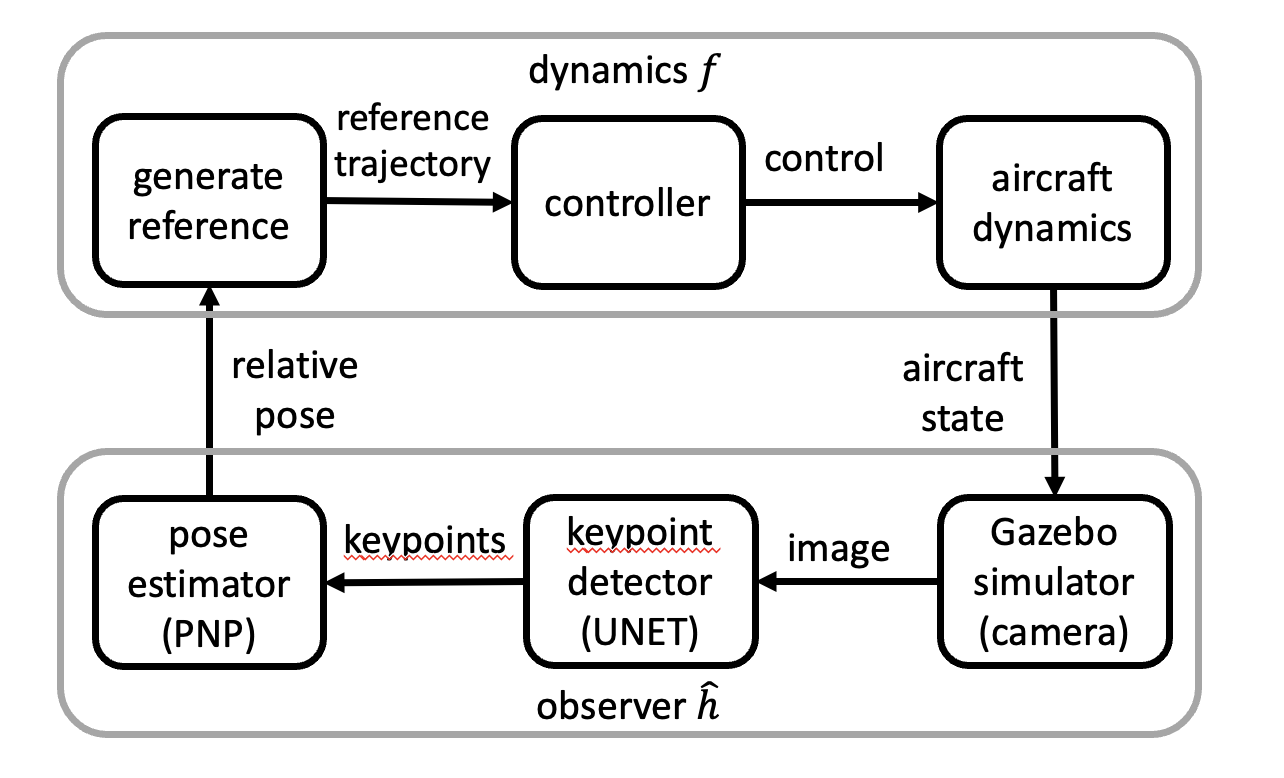
Our first case study is , which is a vision-based auto-landing system. Here an aircraft is attempting to touchdown on a runway using a vision-based pose estimator. Such systems are being contemplated for different types of aircraft landing in airports that do not have expensive Instrumented Landing Systems (ILS). The system block diagram is shown in Fig. 1. The safety requirement defines a sequence of shrinking rectangular regions that the aircraft should remain in (see Fig. 2), otherwise, it has to trigger an expensive missed approach protocol. For our analysis we built a detailed simulation of the aircraft dynamics; the observer or the perception pipeline is the actual code used for vision-based pose estimation.
5.1 AutoLand control system with DNN-based pose estimator
The state space of the AutoLand system is defined by the state variables , where are position coordinates, is the yaw, is the pitch and is the velocity of the aircraft. The perception pipeline implements the observer that attempts to estimate the full state of the aircraft (relative to the touchdown point), except the velocity. That is, the observation space is defined by .
Dynamics.
The dynamics () combines the physics model of the aircraft with a controller that follows a nominal trajectory. A 6-dimensional nonlinear differential equation describes the motion of the aircraft with yaw rate , the pitch rate , and acceleration as the control inputs (Details are given in the Appendix). The aircraft controller tries to follow a reference trajectory approaching the runway. This reference approach trajectory starts at position kilometers from the touchdown point and meters above ground, and has a slope in the z direction. The reference approach has constant speed of .
Vision-based observer.
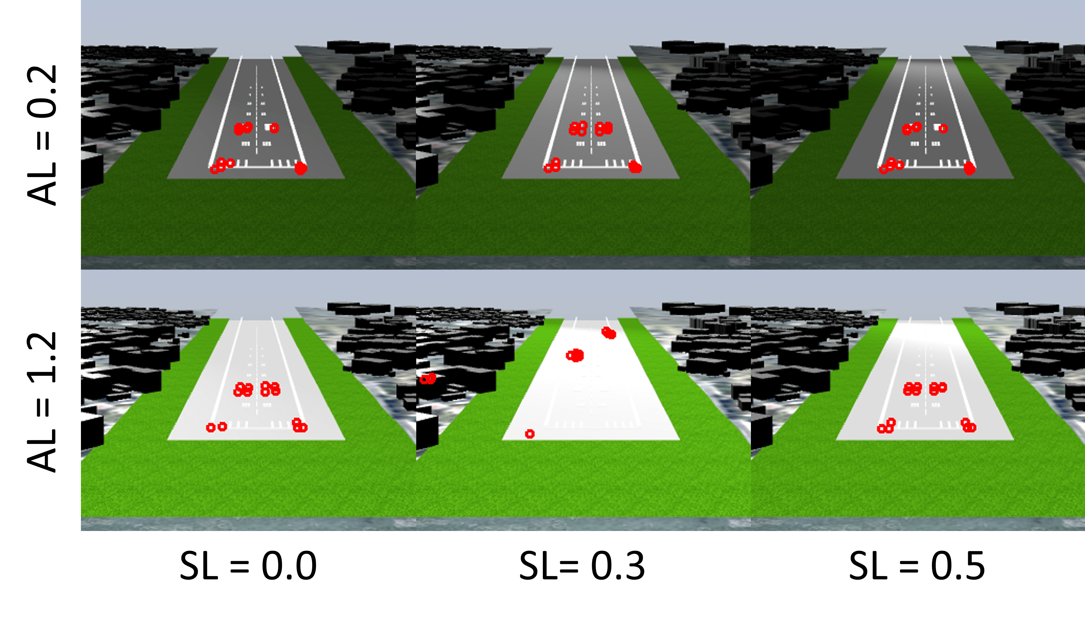
The observations are computed using a realistic perception pipeline composed of three functions (Fig. 1): (1) The airplane’s front camera generates an image, (2) a key-point detector detects specific key-points on the runway in that image using U-Net [20], (3) pose estimator uses the detected key-points and the prior knowledge of the actual positions of those key-points on the ground, to estimate the pose of the aircraft. This last calculation is implemented using the perspective-n-point algorithm [10]. Apart from the impact of the environment on the image, the observer is deterministic.
Environment.
For this paper, we study the effects of two dominant environment factors, namely the ambient light and the position of the sun, represented by a spotlight111We have also performed similar analysis with fog and rain, but the discussion is not included here owing to limited space.. (1) The ambient light intensity in the range [0.2, 1.2] and (2) the spot light’s angle (with respect to the runway) in the range radians, define the environment . These ranges are chosen to include a nominal environment in which there exists an initial state from which the system is safe. Sample camera images from the same state under different environmental conditions are shown in Fig. 1.
5.2 Safety Analysis of AutoLand
We apply DaRePC on the system with reachability analysis implemented using Verse [16]. We run the algorithm with the above range of the environment , the requirement , and on two rectangular initial sets and with different range of initial positions (see Appendix 0.F).
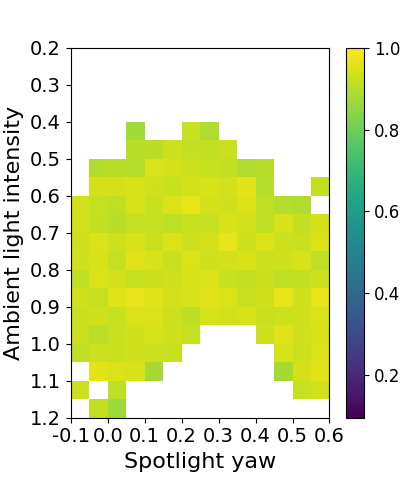
For , the algorithm finds and a corresponding perception contract such that after performing 12 rounds of refinements with empirical conformance measure of . The resulting is visualized in Fig. 2. The white region represents the environmental parameters that are removed (not provably safe) during refinement. For the colored region, different colors represent the empirical conformance of to over each environmental parameter partition. We have following observations from the analysis.
The computed perception contract achieves desired conformance.
To compute the perception contract, we choose the desired conformance , the gap between actual conformance and empirical conformance and the confidence parameter . From LearnContract, the empirical conformance measure should be at least for approximately K samples. We round this up to k samples. The computed perception contract achieves empirical conformance measure over .
Additionally, we run 30 random simulations from under . Out of the resulting K data points generated, observations were contained in the computed perception contract , which gives an empirical conformance of for this different sampling distribution. This shows that meets the desired conformance and can be even better for some realistic sampling distributions.
DaRePC captures interesting behavior.
The set of environmental parameters found by DaRePC also reveals some interesting behavior of the perception pipeline. We can see from Fig. 2 that when the intensity of ambient light is below 0.6 or above 1.15, the performance of perception pipeline becomes bad as many of the partitions are removed in those region. However, we can see there is a region where the ambient lighting condition is close to the nominal ambient lighting condition, but surprisingly, the performance of perception pipeline is still bad. We found that this happens because in this environment, the glare from the spotlight (sun) makes the runway too bright for the perception pipeline to detect keypoints. Conversely, in region , the relatively low ambient light is compensated by the sun, and therefore, the perception pipeline has reliable performance for landing.
Conformance, correctness and system-level safety.
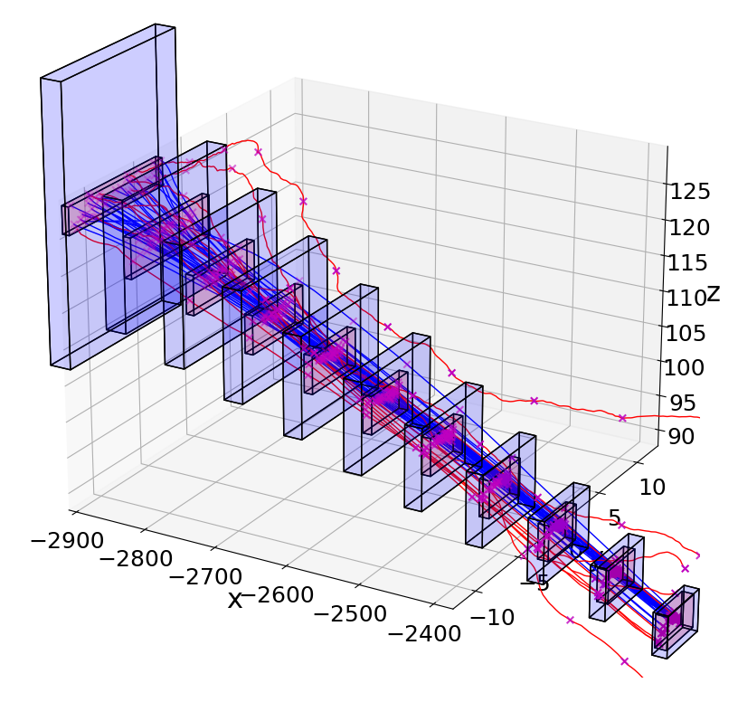
Fig. 2 shows the system-level safety requirement in blue and in red. We can see that the computed reachable set indeed falls inside , which by Proposition 1, implies that if the perception pipeline conforms to then .
Further, to check , we run 30 simulations starting from states randomly sampled from under environments randomly sampled from . The results are shown in Fig. 2. All 30 simulations satisfy , and only one of these is not in the computed reachable set. This happens because doesn’t have conformance, and therefore cannot capture all behaviors of the actual system.
Discovering bad environments; doesn’t satisfy .
We performed 10 random simulations from under . Eight out of the 10 violate (Red trajectories in Fig. 2). This suggests that the environments removed during refinement can indeed lead to real counter-examples violating .
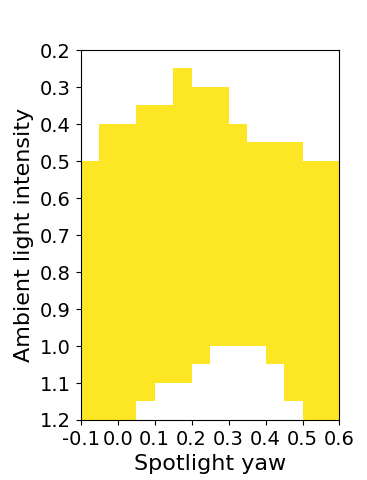
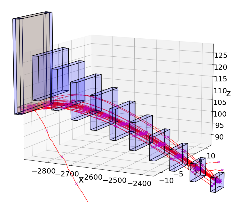
For , DaRePC is able to find a set of states and such that . and are found by calling RefineState on 5 times and ShrinkEnv on 8 times. The computed set of environmental parameters and is shown in Fig. 3. We perform 30 simulations starting from randomly sampled under and the results are shown in Fig. 3. We can see clearly from the plot that all the simulation trajectories violates , which provides evidence that and we found are indeed counter-examples.
5.3 Convergence and conformance of Perception Contracts
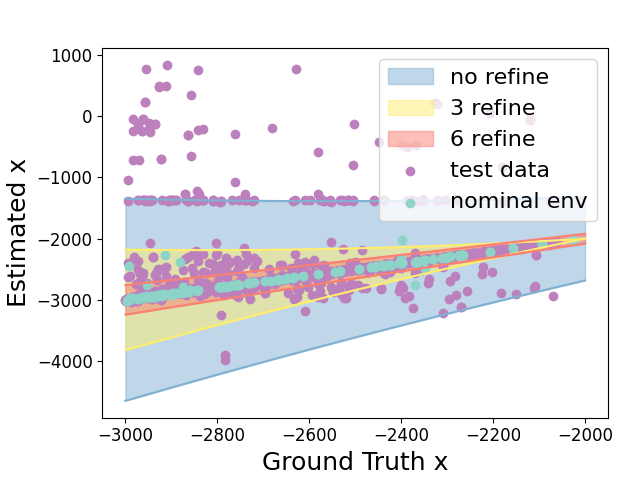
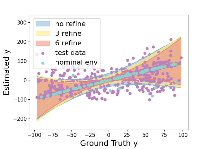
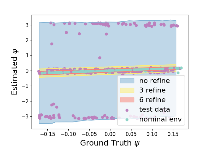
In Section 4.1 , for showing termination of the algorithm, we assume that the perception contract we computed is convergent, i.e. as candidate contracts are computed for a sequence of environments converging to , the contracts also converge to (pointwise). To test this, we pre-sampled k data points and set , . We reduce for by invoking ShrinkEnv function 0, 3, and 6 times on the set of environments with pre-sampled data points. ShrinkEnv refines the environments by removing environmental parameters where the perceived states is far from the actual states and removing corresponding data points sampled under these environments. Fig. 4 shows how the output perception contract and its conformance measure are influenced by successive refinements. For the three range of environments , , after 0,3,6 round of refinements, we observe that , which provides evidence that the perception contract is convergent.
Refinement preserves conformance measure of perception contract.
As we reduce the range of environmental parameters with 0, 3 and 6 refinements, the training data set reduced from 80000 to 71215 and 62638, respectively. Therefore, according to Proposition 2, the empirical conformance measure should at least be for all these three cases to achieve the actual conformance measure. In practice, we are able to get , and empirical conformance measure. From this, we can see refinement preserves conformance measure of perception contract.
6 Case Study: Vision-based Drone Racing (DroneRace)
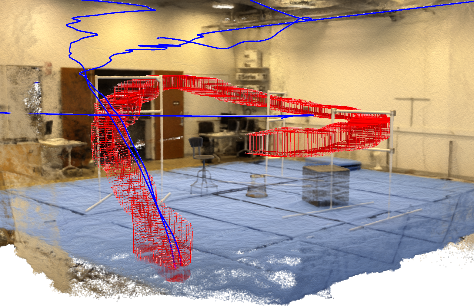
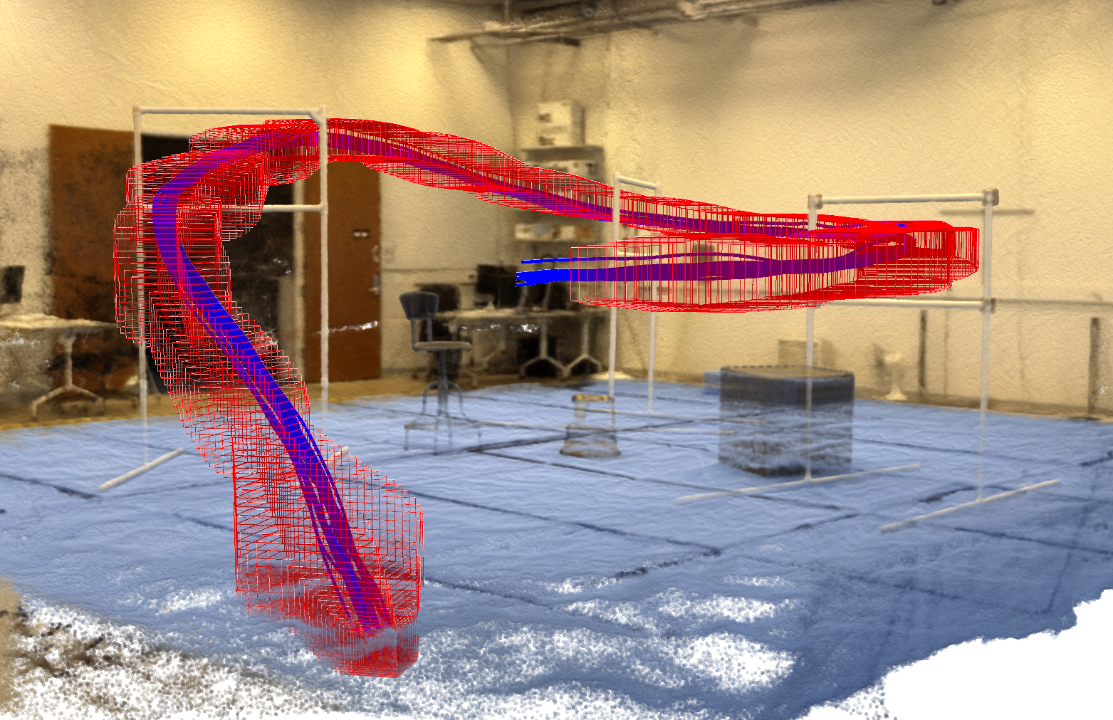
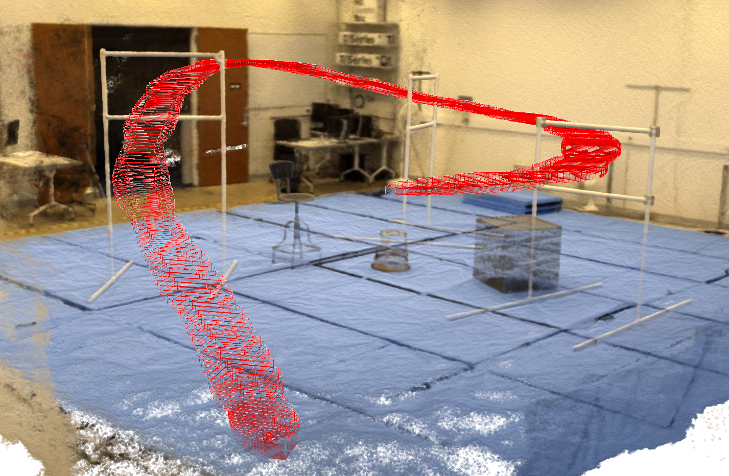
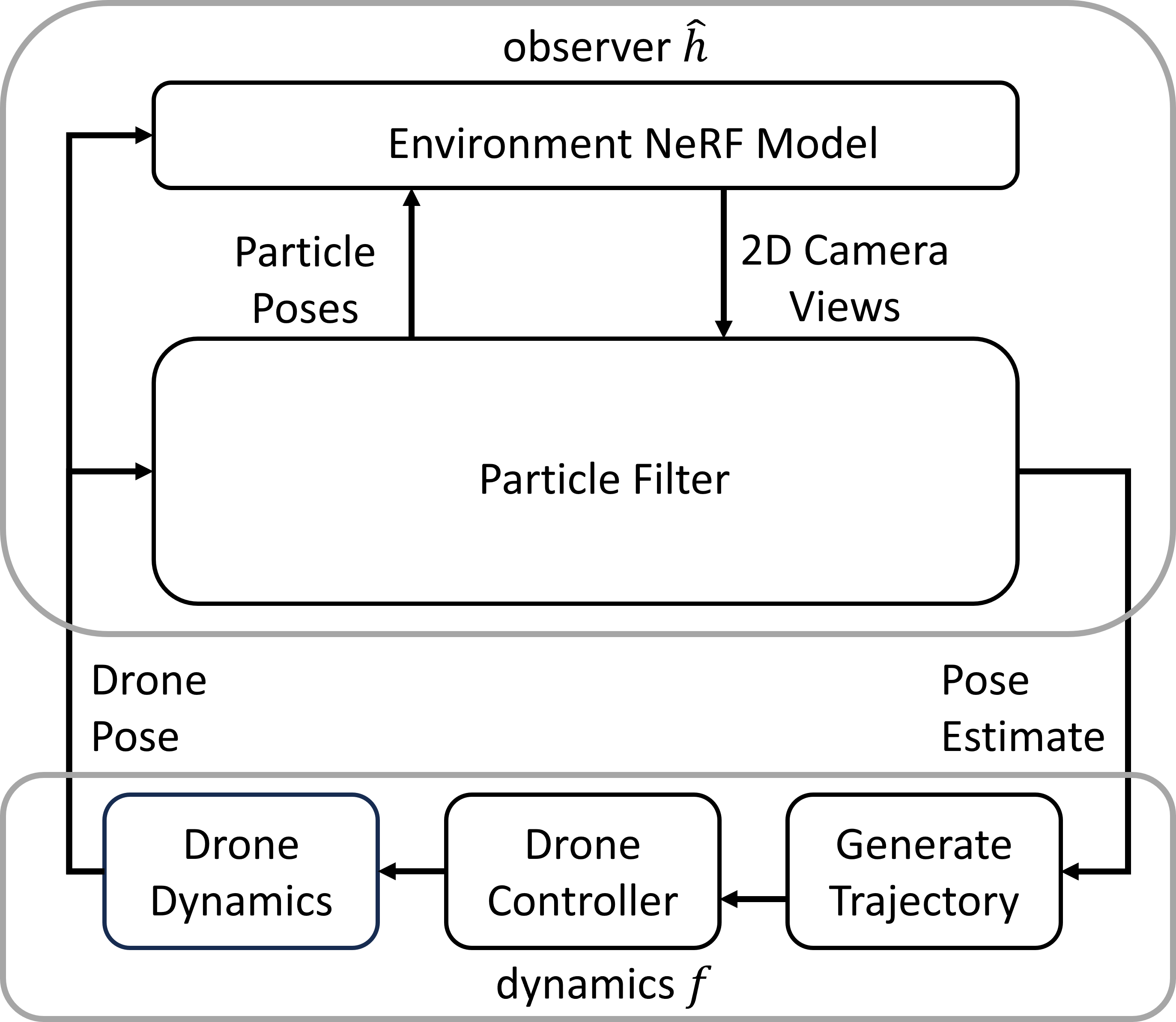
In the second case study, a custom-made quadrotor has to follow a path through a sequence of gates in our laboratory using a vision-based particle filtering for pose estimation. The system architecture is shown in Fig. 6. The safety requirement is a pipe-like region in space passing through the gates. Our analysis here is based on a simulator mimicking the laboratory flying space that we created for this work using Neural Radiance Fields (NeRF) [26]. This simulator enables us to render photo-realistic camera images from any position in the space and with different lighting and visibility (fog) conditions. The observer implementing the vision-based particle filter is the actual code that flies the drone.
6.1 System Description
The 12-dimensional state space of the system is defined by the position , linear velocities , roll pith yaw angles , and the corresponding angular velocities . The observer estimates the 3d-position and the yaw angle. That is, the observation space is defined by . This is a reasonable setup as roll and pitch angles can be measured directly using onboard accelerometer, but position and yaw angles have to be obtained through computation or expensive external devices such as GPS or Vicon.
Dynamics.
A standard 12-dimensional nonlinear model for the drone is used [12]. The input to the aircraft are the desired roll, pitch, yaw angles, and the vertical thrust. The path for passing through the gates is generated by a planner and the controller tries to follow this planned path. More details about the controller and the dynamics are provided in the Appendix 0.H.
Observer.
The observations are computed using a particle filter algorithm from [17]. This is a very different perception pipeline compared to . The probability distribution over the state is represented using a set of particles, from which the mean estimate is calculated. Roughly, the particle filter updates the particles in two steps: in the prediction step it uses the dynamics model to move the particles forward in time, and in the correction step it re-samples the particles to select those particles that are consistent with the actual measurement (images in this case). The details of this algorithm are not important for our analysis. However, it is important to note that the particles used for prediction and correction do not have access to the environment parameters (e.g. lighting).
Besides using current image, the particle filter also uses history information to help estimation and therefore the estimation accuracy may improve over time. The shape of the reference trajectory that the drone is following can also influence its the performance, especially rapid turning in the reference trajectory. Therefore, consider this specific application, we decided to sample data along the reference trajectory for constructing the perception contract which gives similar distribution when the drone is following the reference trajectory.
Environment.
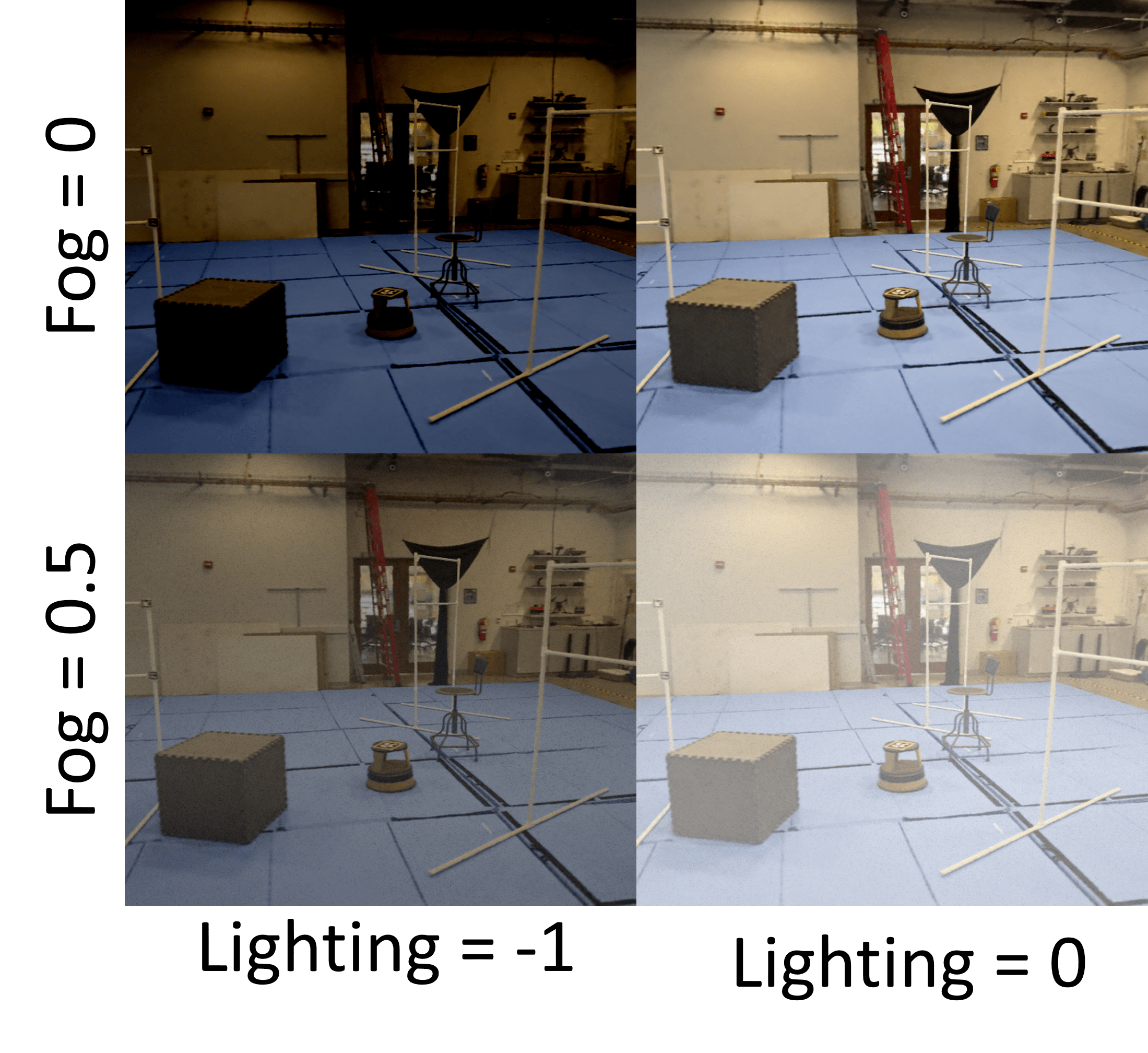
We study the impact of two environmental parameters: (1) Fog ranging from (clear) to (heavy fog), and (2) Ambient light ranging from (dark) and 0 (bright). The nominal environment is a scenario in which the drone is able to complete the path successfully. The effect of different environments on the same view are shown in Fig. 1.
6.2 Analysis of DroneRace
For the DroneRace system, the initial set with , , , , , defines an approach zone (all the other dimensions are set to ). Due to the fact that the perception pipeline for the DroneRace example is highly sensitive, we choose desired actual conformance measure , the gap and the confidence parameter . Therefore, the empirical conformance measure should be at least with at least 5756 training data points.
Conformance, correctness and system-level safety.
For , with 23 refinements on the environmental, DaRePC is able to show that is safe. The environment set that was proved safe is ball-like region around nominal environment . The empirical conformance measure of the contract is , which is higher than the minimal empirical conformance needed to get the desired conformance with confidence . The computed reachable set shows correctness with respect to the requirement (Fig. 5), that is, .
satisfies .
We run 20 random simulated trajectories starting from randomly sampled and . The results are visualized by the blue trajectories in Fig. 5. We can see all the 20 simulations are covered by the Reach computed and therefore doesn’t violate . This provides evidence that the . We also measure the empirical conformance measure of the perception contract for states in these 20 random simulations and the contract is able to get empirical conformance measure on these states.
Discovering bad environments.
We run 20 additional simulations starting from randomly sampled under environments randomly sampled from outside of . The results are shown in Fig. 7 in appendix. We observe that among all 20 simulations, the drone violates requirments in 19 simulations. This provides evidence that the system can easily violate the requirement outside the environmental factors DaRePC identified.
7 Discussions
There are several limitations of the perception contract method developed in this paper, which also suggest directions for future explorations.
Distributional Shifts.
We discussed that DaRePC has nice properties of conformance and termination provided LearnContract converges, as the environment converges to the ground conditions. This only makes sense in the limited situation where the underlying sampling distribution for constructing the contract remains the same under deployed conditions. It will be important to develop techniques for detecting and adapting to distributional shifts in the perception data, in order to have guarantees that are robust to such changes [1].
Runtime monitoring and control.
The proplem formulation in this paper is focused on verification, which in turn requires the identification of the environmental conditions under which system safety can be assured. Perception contracts can also be used for runtime monitoring for detection of the violation of certain properties. The key challenge here is to compute preimages of the contracts, that is: , that can be used for detecting violation or imminent violation of the requirements. Another related problem is the correction of such imminent violations by changing the control actions.
The paper presents the analysis of 6 and 12 dimensional flight control systems that use multi-stage, heterogeneous, ML-enabled perception. Both systems have high-dimensional nonlinear dynamics and realistic perception pipelines including deep neural networks. We explore how the variation of environment impacts system level safety performance. We advances the method of perception contract by introducing an algorithm for constructing data and requirement guided refinement of perception contracts (DaRePC). DaRePC is able to either identify a set of states and environmental factors that the requirement can be satisfied or find a counter example. In future, we are planning to apply the algorithm to real hardware to test its performance.
References
- [1] Amodei, D., Olah, C., Steinhardt, J., Christiano, P., Schulman, J., Mané, D.: Concrete problems in ai safety (2016)
- [2] Angello, A., Hsieh, C., Madhusudan, P., Mitra, S.: Perception contracts for safety of ml-enabled systems. In: Proc. of the ACM on Programming Languages (PACMPL), OOPSLA (2023)
- [3] Calinescu, R., Imrie, C., Mangal, R., Rodrigues, G.N., Păsăreanu, C., Santana, M.A., Vázquez, G.: Discrete-event controller synthesis for autonomous systems with deep-learning perception components. arXiv:2202.03360 (2023)
- [4] Dean, S., Matni, N., Recht, B., Ye, V.: Robust guarantees for perception-based control. In: Bayen, A.M., Jadbabaie, A., Pappas, G., Parrilo, P.A., Recht, B., Tomlin, C., Zeilinger, M. (eds.) Proceedings of the 2nd Conference on Learning for Dynamics and Control. Proceedings of Machine Learning Research, vol. 120, pp. 350–360. PMLR (10–11 Jun 2020), https://proceedings.mlr.press/v120/dean20a.html
- [5] Dean, S., Taylor, A., Cosner, R., Recht, B., Ames, A.: Guaranteeing safety of learned perception modules via measurement-robust control barrier functions. In: Kober, J., Ramos, F., Tomlin, C. (eds.) Proceedings of the 2020 Conference on Robot Learning. Proceedings of Machine Learning Research, vol. 155, pp. 654–670. PMLR (16–18 Nov 2021), https://proceedings.mlr.press/v155/dean21a.html
- [6] Dekkers, G.: Quantile regression: Theory and applications (2014)
- [7] Dreossi, T., Fremont, D.J., Ghosh, S., Kim, E., Ravanbakhsh, H., Vazquez-Chanlatte, M., Seshia, S.A.: VerifAI: A toolkit for the formal design and analysis of artificial intelligence-based systems. In: Computer Aided Verification (CAV) (Jul 2019)
- [8] Everett, M., Habibi, G., How, J.P.: Efficient reachability analysis of closed-loop systems with neural network controllers. In: 2021 IEEE International Conference on Robotics and Automation (ICRA). pp. 4384–4390 (2021). https://doi.org/10.1109/ICRA48506.2021.9561348
- [9] Fan, C., Qi, B., Mitra, S., Viswanathan, M.: Dryvr: Data-driven verification and compositional reasoning for automotive systems. In: Majumdar, R., Kunčak, V. (eds.) Computer Aided Verification (CAV). pp. 441–461. Springer, Cham (2017)
- [10] Fischler, M.A., Bolles, R.C.: Random sample consensus: A paradigm for model fitting with applications to image analysis and automated cartography. Commun. ACM 24(6), 381–395 (jun 1981). https://doi.org/10.1145/358669.358692, https://doi.org/10.1145/358669.358692
- [11] Fremont, D.J., Chiu, J., Margineantu, D.D., Osipychev, D., Seshia, S.A.: Formal analysis and redesign of a neural network-based aircraft taxiing system with VerifAI. In: Computer Aided Verification (CAV) (Jul 2020)
- [12] Herbert, S.L., Chen, M., Han, S., Bansal, S., Fisac, J.F., Tomlin, C.J.: Fastrack: A modular framework for fast and guaranteed safe motion planning. In: 2017 IEEE 56th Annual Conference on Decision and Control (CDC). pp. 1517–1522 (2017). https://doi.org/10.1109/CDC.2017.8263867
- [13] Hoeffding, W.: Probability inequalities for sums of bounded random variables. Journal of the American Statistical Association 58(301), 13–30 (1963), http://www.jstor.org/stable/2282952
- [14] Hsieh, C., Koh, Y., Li, Y., Mitra, S.: Assuring safety of vision-based swarm formation control (2023)
- [15] Hsieh, C., Li, Y., Sun, D., Joshi, K., Misailovic, S., Mitra, S.: Verifying controllers with vision-based perception using safe approximate abstractions. IEEE Transactions on Computer-Aided Design of Integrated Circuits and Systems 41(11), 4205–4216 (2022)
- [16] Li, Y., Zhu, H., Braught, K., Shen, K., Mitra, S.: Verse: A python library for reasoning about multi-agent hybrid system scenarios. In: Enea, C., Lal, A. (eds.) Computer Aided Verification. pp. 351–364. Springer Nature Switzerland, Cham (2023)
- [17] Maggio, D., Abate, M., Shi, J., Mario, C., Carlone, L.: Loc-nerf: Monte carlo localization using neural radiance fields (2022)
- [18] Păsăreanu, C.S., Mangal, R., Gopinath, D., Getir Yaman, S., Imrie, C., Calinescu, R., Yu, H.: Closed-loop analysis of vision-based autonomous systems: A case study. In: Proc. 35th Int. Conf. Comput. Aided Verification. pp. 289–303 (2023)
- [19] Păsăreanu, C., Mangal, R., Gopinath, D., Yu, H.: Assumption Generation for the Verification of Learning-Enabled Autonomous Systems. arXiv:2305.18372 (2023)
- [20] Ronneberger, O., Fischer, P., Brox, T.: U-net: Convolutional networks for biomedical image segmentation. In: Navab, N., Hornegger, J., Wells, W.M., Frangi, A.F. (eds.) Medical Image Computing and Computer-Assisted Intervention – MICCAI 2015. pp. 234–241. Springer International Publishing, Cham (2015)
- [21] Santa Cruz, U., Shoukry, Y.: Nnlander-verif: A neural network formal verification framework for vision-based autonomous aircraft landing. In: Deshmukh, J.V., Havelund, K., Perez, I. (eds.) NASA Formal Methods. pp. 213–230. Springer International Publishing, Cham (2022)
- [22] Shoouri, S., Jalili, S., Xu, J., Gallagher, I., Zhang, Y., Wilhelm, J., Jeannin, J.B., Ozay, N.: Falsification of a Vision-based Automatic Landing System. https://doi.org/10.2514/6.2021-0998, https://arc.aiaa.org/doi/abs/10.2514/6.2021-0998
- [23] Song, Y., Romero, A., Müller, M., Koltun, V., Scaramuzza, D.: Reaching the limit in autonomous racing: Optimal control versus reinforcement learning. Science Robotics 8(82), eadg1462 (2023). https://doi.org/10.1126/scirobotics.adg1462, https://www.science.org/doi/abs/10.1126/scirobotics.adg1462
- [24] Sun, D., Mitra, S.: NeuReach: Learning reachability functions from simulations. In: Fisman, D., Rosu, G. (eds.) Tools and Algorithms for the Construction and Analysis of Systems. pp. 322–337. Springer, Cham (2022)
- [25] Sun, D., Yang, B.C., Mitra, S.: Learning-based perception contracts and applications (2023)
- [26] Tancik, M., Weber, E., Ng, E., Li, R., Yi, B., Kerr, J., Wang, T., Kristoffersen, A., Austin, J., Salahi, K., Ahuja, A., McAllister, D., Kanazawa, A.: Nerfstudio: A modular framework for neural radiance field development. In: ACM SIGGRAPH 2023 Conference Proceedings. SIGGRAPH ’23 (2023)
Appendix 0.A Proof for Proposition 1
Proposition 1 Restated Suppose contains the reachable states of the system . If is a -perception contract for for some requirement , then satisfies , i.e., .
Proof
Consider any environment , any initial state . From correctness of , it follows that . That is, for the system with as observer the reachable sets for all , and for each . Now consider any execution of . We know . Since , from conformance of , we know that for all . Therefore, for , we have . This tells us that for all execution for all , which gives us .
Appendix 0.B Proof for Proposition 2
Proposition 2 Restated For any , with probability at least , we have that
Proof
From Hoeffding’s inequality, we get
This implies that
which proves the proposition.
Appendix 0.C Proof for Proposition 3
Proposition 3 Restated Given , and an execution of in nominal environment , , such that generated by calling RefineState times on and obtained on environment refined by ShrinkEnv times satisfies that ,
Proof
We know from the definition of ShrinkEnv that as the sequence of sets of environmental parameters generated by ShrinkEnv will monotonically converge to a singleton set contain the grounding environmental parameter . We know from convergence of that will converge to as the set of environmental parameters converge to a singleton set. In addition, we know the output of RefineState will converge to a singleton set of states after it’s repeatedly invoked by definition. Therefore, by the assumption of Reach, when a partition converges to some and , which is the trajectory starting from state generated by under environmental parameter .
Appendix 0.D Proof for Theorem 4.2
Theorem 4.2 Restated If satisfies conformance and convergence and satisfy/violate requirement robustly, then Algorithm 2 always terminates, i.e., the algorithm can either find a and that or find a counter-example and with that .
Proof
To show completeness of the algorithm, we need to show four cases:
1) When there exist a counter-example, the algorithm can find the counter-example. If there exist a counter-example such that trajectory starting from under grounding environmental parameter exits at time , then according to the robustness assumption of the system, there exist , such that , . Therefore, according to Proposition 3, with enough refinement, we can get a set of states with and with such that . In this case, which captures the counter-example.
2) A counter-example returned is indeed a counter-example. A set of states is returned as counter-example when , such that for some . From conformance of , we know for all and In this case, trajectory starting from with any environmental parameter will satisfy that which is not in . The output of DaRePC in this case is indeed a counter-example.
3) When a counter-example doesn’t exist, the algorithm can find satisfy on . This case can be shown similar to case 1). Since we assume the system is robust, for every trajectory of the system that satisfies , there exist such that for all . Since we know as DaRePC repeatedly performs refinement, will converge to a single execution. Therefore, according to Proposition 3, with enough refinement, for all safe trajectory we can get . Therefore, with enough refinement, we can always find a that satisfies when the satisfy on under .
4) A returned by DaRePC will always satisfy on . This is given automatically by Theorem 4.1 and the conformance assumption.
Appendix 0.E Dynamics and Controller for AutoLand Case Study
The dynamics of the AutoLand Case Study is given by
is a descretization parameter. The control inputs are the yaw rate , pitch rate and acceleration
The error between the reference points and state is then given by
The control inputs are then computed using errors computed by a PD controller.
Appendix 0.F Initial Sets for AutoLand Case Study
The initial sets , for AutoLand case study are
Appendix 0.G Block Diagram for DroneRace
The block diagram for the DroneRace case study is shown in Fig. 6
Appendix 0.H Dynamics and Controller for DroneRace Case Study
We used a slightly modified version of drone dynamics from [12]. It’s given by the following differential equations
Where some parameters , , , , . Given reference state provided by the reference trajectory, we can compute the tracking error between reference state and current state . The position error between current state of the drone and the reference trajectory is given by.
The tracking error for other states is given by the difference between reference state and current state. Therefore, the control signals can be computed using following feedback controller.
Appendix 0.I Simulation Trajectories for for DroneRace