Refined Belief-Propagation Decoding of Quantum Codes with Scalar Messages
Abstract
Codes based on sparse matrices have good performance and can be efficiently decoded by belief-propagation (BP). Decoding binary stabilizer codes needs a quaternary BP for (additive) codes over GF(4), which has a higher check-node complexity compared to a binary BP for codes over GF(2). Moreover, BP decoding of stabilizer codes suffers a performance loss from the short cycles in the underlying Tanner graph. In this paper, we propose a refined BP algorithm for decoding quantum codes by passing scalar messages. For a given error syndrome, this algorithm decodes to the same output as the conventional quaternary BP but with a check-node complexity the same as binary BP. As every message is a scalar, the message normalization can be naturally applied to improve the performance. Another observation is that the message-update schedule affects the BP decoding performance against short cycles. We show that running BP with message normalization according to a serial schedule (or other schedules) may significantly improve the decoding performance and error-floor in computer simulation.
Index Terms:
Quantum stabilizer codes, LDPC codes, sparse matrices, belief-propagation, sum-product algorithm, message-update schedule, message normalization.I Introduction
In the 1960s, Gallager proposed the low-density parity-check (LDPC) codes (or called sparse codes) and sum-product (decoding) algorithm to have a near Shannon-capacity performance for many channels, including the binary symmetric channel (BSC) and additive white Gaussian noise (AWGN) channel [1, 2, 3, 4, 5]. The sum-product algorithm runs an iterative message-passing on the Tanner graph [6] defined by a parity-check matrix of the code [7, 8, 9], where the procedure is usually understood as a realization of Pearl’s belief-propagation (BP)—a widely-used algorithm in machine-learning and artificial-intelligence [10, 11, 12].
The parity-check matrix of a classical code is used to do syndrome measurements for (syndrome-based) decoding. In the 1990s, quantum error-correction was proposed to be done in a similar way by using stabilizer codes [13, 14, 15, 16, 17]. There will be a check matrix defined for a stabilizer code to do the projective (syndrome) measurements for decoding. Many sparse stabilizer codes have been proposed, such as topological codes [18, 19], random sparse codes (in particular, bicycle codes) [20], and hypergraph-product codes [21].
Decoding a binary stabilizer code is equivalent to decoding an additive code over GF() (representing Pauli errors ) [17]. That is, a quaternary BP (BP4) is required, with every message conventionally a length-four vector to represent a distribution over GF(4). In contrast, decoding a binary classical code only needs a binary BP (BP2), with every message a scalar (e.g., as a log-likelihood ratio (LLR) [2] or likelihood difference (LD) [5]). As a result, BP2 has a check-node efficiency times better than the conventional BP4 [22].111 The complexity can be for the fast Fourier transform (FFT) method [23, 24]. But a comparison based on this is more suitable for a larger , since there is additional cost running FFT and inverse FFT. To reduce the complexity, it often treats a binary stabilizer code as a binary classical code with doubled length so that BP2 can be used [20], followed by additional processes to handle the / correlations [25, 26].
A stabilizer code inevitably has many four-cycles in its Tanner graph, which degrade the performance of BP [20, 27]. To improve, additional pre/post-processes are usually used, such as heuristic flipping from nonzero syndrome bits [27], (modified) enhanced-feedback [28, 29], training a neural BP [30], augmented decoder (adding redundant rows to the check matrix) [26], and ordered statistics decoding (OSD) [31].
In this paper, we first simplify the conventional BP4. An important observation is that, though a binary stabilizer code is considered as a quaternary code, its error syndrome is binary. Inspired by this observation and MacKay’s LD-based computation rule (-rule) (cf. (47)–(53) in [5]), we derive a -rule based BP4 that is equivalent to the conventional BP4 but passing every message as a scalar, which improves the check-node efficiency 16 times and does not need additional processes to handle the / correlations.
Then we improve BP4 by introducing classical BP techniques. First, the messages can be updated in different orders (schedules) [32, 33, 34]. Second, as we have scalar messages, the message normalization can be applied [35, 36, 37]. With these techniques, our (scalar-based) BP4 shows a much improved empirical performance in computer simulation.
II Classical Binary Belief-Propagation Decoding
II-A The notation and parallel/serial BP2
We consider the syndrome-based decoding. Consider an classical binary linear code defined by an parity-check matrix (not necessarily of full rank) with . Upon the reception of a noisy codeword disturbed by an unknown error , syndrome measurements (defined by rows of ) are performed to generate a syndrome vector . The decoder is given , , and an a priori distribution for each to infer an such that the probability is as high as possible.222 Giving can be according to a channel model [5] or even a fixed distribution (useful if the channel parameter is unknown) [38]. Here, we uses the former case since it usually has a better performance. BP decoding is done by updating each as an a posterior distribution and inferring by . This is done by doing an iterative message-passing on the Tanner graph defined by .
The Tanner graph corresponding to is a bipartite graph consisting of variable nodes and check nodes, and there is an edge connecting check node and variable node if entry . Let be row of . An example Tanner graph of is shown in Fig. 1.
For the iterative message-passing, there will be a variable-to-check message and a check-to-variable message passed on edge . Let and . (And we will write things like as to simplify the notation.) Assume that every initially. An iteration is done by:
-
•
is computed by with ,
-
•
is computed by with ,
-
•
is computed by with .
The messages and will be denoted, respectively, by and for simplicity. The message-passing is usually done with a parallel schedule, referred to as parallel BP2 (cf. [39, Algorithm 1], which has and as likelihood differences (LDs) and is due to MacKay and Neal [3, 4, 5]).
II-B The simplified rules for BP2
The computation in parallel/serial BP2 can be substantially simplified and represented by simple update rules, corresponding to weight-2 and weight-3 rows. These simple rules can in turn be extended to define the general rules [9, Sec. V-E]. Consider as in Fig. 1. Recall that we denote and . Let be a super bit indexed by . Then we have the representation and . By Bayes rule and some derivations, we can update the (conditional) distribution of , say , by:
LD-rule (-rule)
The distribution of can be updated by (conditions) and , respectively, by:
| (1) | ||||
where
| (2) | ||||
where is the likelihood difference (LD) of ,
| (3) |
We describe the -rule following [5] rather than [9]. This allows us to generalize the computation to the quantum case later. The -rule is equivalent to the LLR-rule as follows.
LLR-rule (-rule)
Let be the log-likelihood ratio (LLR) of . Define like what Gallager did [1], where , , and . (Note that .) The LLR of can be updated by (conditions) and , respectively, by:
where is defined by
| (4) |
It only needs an addition after a transform by . To prevent handling the signs separately, it can use a transform by but needs a multiplication [40] by
| (5) |
Using simple algebra can confirm that the in (4) and (5) are equivalent, and for the and defined in (2). More equivalent rules can be found in [9, Sec. V-E].
Depending on the application (the channel model, decoder hardware, etc.), a suitable rule can be chosen. For example, the -rule is suitable for the AWGN channel (since the received symbol’s magnitude is linearly mapped to [2]), and the operation can be efficiently computed/approximated (e.g., by table lookup [36]). On the other hand, the -rule is suitable for the BSC, and the computation can be efficiently programmed/computed by a general-purpose computer.
The -rule is very suitable for our purpose of decoding quantum codes in the next section.
III Quaternary BP Decoding for Quantum Codes
III-A The simplified rule for BP4
We will use the notation based on Pauli operators [41], and consider -fold Pauli operators with an inner product
| (6) |
which has an output 0 if the inputs commute and an output 1 if the inputs anticommute. (This is mathematically equivalent to mapping GF(4)N with a Hermitian trace inner-product to the ground field GF(2) [17]). It suffices to omit in the following discussion. An unknown error will be denoted by .
There will a check matrix used to generate a syndrome . Consider a simple example , where there are five non-identity entries. For simplicity, fix it as and the other cases can be handled similarly. The Tanner graph (with generalized edge types ) of the example is shown in Fig. 2.
For decoding quantum codes, we are to update an initial distribution of as an updated (conditional) distribution . Again (as in Sec. II-B) assume that the syndrome is a zero vector and we are to update the distribution of with . By Bayes rule and some derivations, we have:
LD-rule (-rule) for BP4
The distribution of can be updated by (conditions) and , respectively, by:
| (7) | ||||
where (since )
The last two probabilities (with 16 multiplications as above) can be efficiently computed (with one multiplication) by
| (8) |
where (since and )
| (9) | ||||
Observe the similarity and difference in (1)–(3) and (7)–(9). This even suggests a way to generalize the above strategy to a case of higher-order GF() with binary syndromes.
This pre-add strategy is like a partial FFT-method since for GF(), the basic operation of the ground filed GF(2) is addition (subtraction) [24]. However, the FFT-method needs additions and multiplications to combine two distributions [23]. The above strategy, by generalizing (8) and (9), would only need additions and multiplication to combine two distributions if the syndrome is binary. Another point is that the FFT-method still treats a message as a vector over GF(), but we treat the message as a scalar and this opens new possibilities for improvement (e.g., using message normalization (shown later) or allowing a neural BP4, where (since training needs scalar messages) a previous neural BP is only considered with BP2 without / correlations [30]).
III-B The conventional BP4 with vector messages
An stabilizer code is a -dimensional subspace of fixed by the operators (not necessarily all independent) defined by a check matrix with . Each row of corresponds to an -fold Pauli operator that stabilizes the code space. The matrix is self-orthogonal with respect to the inner product (6), i.e., for any two rows and . The code space is the joint-() eigenspace of the rows of . The vectors in the (multiplicative) rowspace of are called stabilizers [41].
It suffices to consider discrete errors like Pauli errors per the error discretization theorem [41]. Upon the reception of a noisy coded state suffered from an unknown -qubit error , stabilizers are measured to determine a binary error syndrome using (6), where
| (10) |
Given , , and an a priori distribution for each (e.g., let for a depolarizing channel with error rate ), a decoder has to estimate an such that is equivalent to , up to a stabilizer, with a probability as high as possible. (The solution is not unique due to the degeneracy [27, 42].)
For decoding quantum codes, the neighboring sets are and . Let be the restriction of to .
Then for any and .333
For example, if and , then
and . Then
A conventional BP4 for decoding binary stabilizer codes is done as follows [27]. In the initialization step, every variable node passes the message to every neighboring check node .
-
•
Horizontal Step: At check node , compute and pass as the message for every , where ,
-
•
Vertical Step: At variable node , compute and pass as the message for every , where
with a chosen scalar to let .
At variable node , it also computes to infer . The horizontal and vertical steps are iterated until an estimated is valid or a maximum number of iterations is reached.
III-C The refined BP4 with scalar messages
For a variable node, say variable node 1, and its neighboring check node , we know from (10) that
Given the value of (a possible) and some , we will know that commutes or anticommutes with , i.e., either or . Consequently, the passed message should indicate more likely whether or . In other words, the message from a neighboring check will tell us more likely whether the error commutes or anticommutes with . This suggests that a BP decoding of stabilizer codes with scalar messages is possible and we provide such an algorithm in Algorithm 1, referred to as parallel BP4 (the same as [39, Algorithm 3]). Note that the notation is simplified as .
Input: , , and initial .
Initialization. For and , let
where and .
Horizontal Step. For and , compute
Vertical Step. For and , do:
-
•
Compute ,
-
•
Let
and ,
where is a chosen scalar such that . -
•
Update: .
Hard Decision. For , compute
-
Let .
-
•
Let .
-
–
If , halt and return “SUCCESS”;
-
–
otherwise, if a maximum number of iterations is reached, halt and return “FAIL”;
-
–
otherwise, repeat from the horizontal step.
-
–
It can be shown that Algorithm 1 has exactly the same output as the conventional BP4 (as outlined in Sec. III-A). In particular, Algorithm 1 has a check-node efficiency 16-fold improved from the conventional BP4.
Similar to the classical case, we can consider running Algorithm 1 with a serial schedule, referred to as serial BP4 (cf. [39, Algorithm 4]). Using serial BP4 may prevent the decoding oscillation (as an example based on the code in [39, Fig. 7]) and improve the empirical performance (e.g., for decoding a hypergraph-product code [39, Fig. 8]).
IV Simulation Results
Identical to Algorithm 1, except that and are respectively replaced by and for some , where is a chosen scalar such that .
Having scalar messages allows us to apply the message normalization [35, 36, 37]. This suppresses the wrong belief looped in the short cycles (due to sub-matrices like in Fig. 2). The message normalization can be applied to [39, Algorithm 5] or [39, Algorithm 6]. Many simulation results were provided in [39], and normalizing has a lower error-floor. We restate [39, Algorithm 6] as Algorithm 2 here (where can be efficiently done by one multiplication and two additions [43]). Some more results will be provided. We try to collect at least 100 logical errors for every data-point; or otherwise an error bar between two crosses shows a 95% confidence interval (omitted in Fig. 6).
In the simulation, we do not restrict the measurements to be local. We consider bicycle codes (a kind of random sparse codes) [20] since they have small ancilla overhead and good performance, benchmarked by code rate vs. physical error rate [20, Fig. 10].444 Using random sparse codes needs long qubit-connectivity, which is possibly supported by trapped-ions or nuclear-spins [44]. If the measurements must be local, then topological codes are usually considered (with another benchmark called threshold usually used). Our proposed algorithm can also decode topological codes but needs some extension to have a good performance. This will be addressed in another our manuscript under preparation. But BP decoding of this kind of codes have some error-floor subject to improve [20, Fig. 6].
First, a random bicycle code is easy to construct [27] but could have a high error-floor [39]. For convenience, we replot [39, Fig. 16] as Fig. 4 here. Observe the high error-floor before using message normalization. Using improves the error-floor a lot. We implemented an overflow (underflow) protection in BP as in [5] and confirmed that the original error-floor is not due to numerical overflow/underflow. It should be due to the random construction (especially that a row-deletion step is performed randomly). MacKay, Mitchison, and McFadden suggested to use a heuristic approach to do the construction (to have more uniform column-weights in the check matrix after the row-deletion step) [20].555 Except for special irregular designs, BP converges more well when the column-weights are more uniform [2, 5, 20]. We consider to either minimize the column-weight variance (min-var approach) or minimize the difference of the largest and smallest column-weights (min-max approach). The min-var approach is usually better; but if many rows are deleted (for a larger code rate), the min-max approach could be better. The code (rate 1/2) constructed here is by the min-max approach. The code (rate 1/4) constructed here is by the min-var approach.
An bicycle code is constructed by the heuristic approach, with the other parameters the same as the code in Fig. 4. The performance of this new code is shown in Fig. 4, where the BP4 error-floor (without message normalization) is improved compare to Fig. 4. However, using further lowers the error-floor to a level like the improved case in Fig. 4. The two figures show that running (scalar-based) BP4 with message normalization has a more robust performance. This provides more flexibility in code construction (for if some rows (measurements) must be kept or deleted).


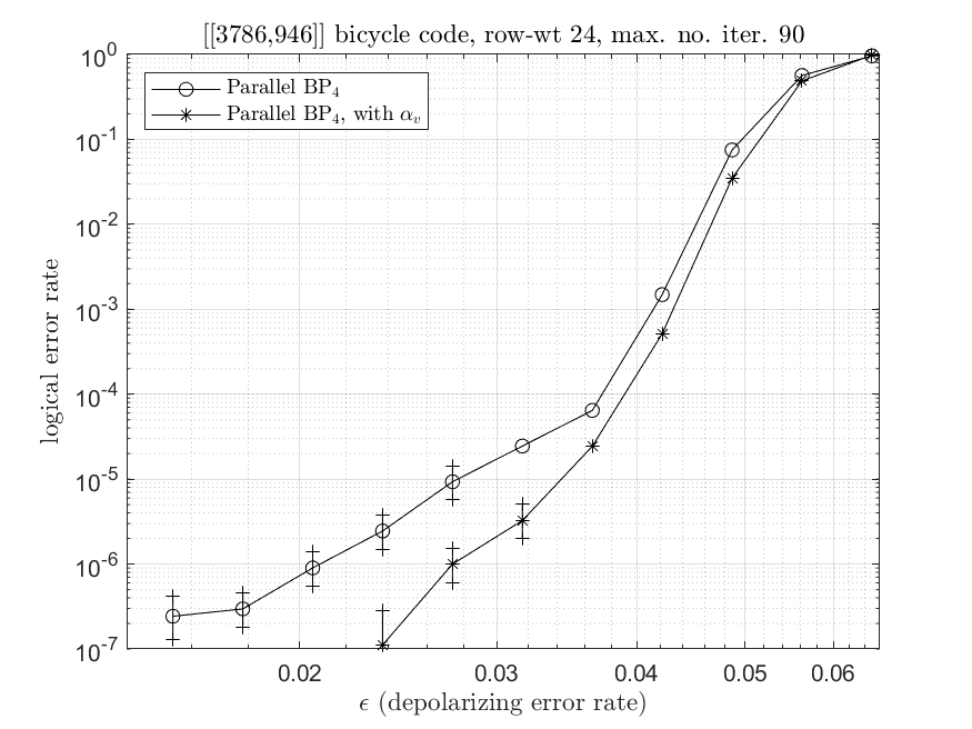
Next we construct a bicycle code with row-weight 24, using the heuristic approach. A code with such parameters has some error-floor for a block error rate , when decoded by BP2 in the bit-flip channel [20, Fig. 6]. We decode the constructed code by BP4 in the depolarizing channel, and plot the decoding performance in Fig. 6. There is a similar error-floor for a logical error rate before using message normalization. After using , the error-floor performance is much improved. A smaller usually needs a larger for suppression (since is quite biased with a large ). As a reference, we derive Fig. 6 from Fig. 6 by using different for different to see the improvement.

V Conclusion
We proposed a -rule based BP4 for decoding quantum stabilizer codes by passing scalar messages. This is achieved by exploiting the binary property of the syndrome. The proposed BP4 is equivalent to the conventional BP4 but with a check-node efficiency 16-fold improved. The message normalization can be naturally applied to the scalar messages. We performed the simulation by decoding several bicycle codes. Different decoding schedules were also considered. Using the proposed BP4 with message normalization and a suitable schedule results in a significantly improved performance and error-floor.
References
- [1] R. G. Gallager, “Low-density parity-check codes,” IRE Transactions on Information Theory, vol. 8, pp. 21–28, 1962.
- [2] ——, Low-Density Parity-Check Codes, ser. no. 21 in Research Monograph Series. Cambridge, MA: MIT Press, 1963.
- [3] D. MacKay and R. Neal, “Good codes based on very sparse matrices,” in Proc. 5th IMA Int. Conf. Cryptogr. Coding, 1995, pp. 100–111.
- [4] ——, “Near Shannon limit performance of low density parity check codes,” Electron. Lett., vol. 32, pp. 1645–1646, 1996, reprinted: Electron. Lett., vol. 33, pp. 457–458, 1997.
- [5] D. J. C. MacKay, “Good error-correcting codes based on very sparse matrices,” IEEE Trans. Inf. Theory, vol. 45, pp. 399–431, 1999.
- [6] R. Tanner, “A recursive approach to low complexity codes,” IEEE Trans. Inf. Theory, vol. 27, pp. 533–547, 1981.
- [7] N. Wiberg, “Codes and decoding on general graphs,” Ph.D. dissertation, Linkoping University, Linkoping, Sweden, 1996.
- [8] S. M. Aji and R. J. McEliece, “The generalized distributive law,” IEEE Trans. Inf. Theory, vol. 46, pp. 325–343, 2000.
- [9] F. Kschischang, B. Frey, and H. Loeliger, “Factor graphs and the sum-product algorithm,” IEEE Trans. Inf. Theory, vol. 47, pp. 498–519, 2001.
- [10] J. Pearl, Probabilistic reasoning in intelligent systems: networks of plausible inference. Morgan Kaufmann, 1988.
- [11] R. J. McEliece, D. J. C. MacKay, and J.-F. Cheng, “Turbo decoding as an instance of Pearl’s “belief propagation” algorithm,” IEEE J. Sel. Areas Commun., vol. 16, pp. 140–152, 1998.
- [12] J. S. Yedidia, W. T. Freeman, and Y. Weiss, “Understanding belief propagation and its generalizations,” Exploring Artif. Intell. in the New Millennium, vol. 8, pp. 236–239, 2003.
- [13] P. W. Shor, “Scheme for reducing decoherence in quantum computer memory,” Phys. Rev. A, vol. 52, pp. 2493–2496, 1995.
- [14] D. Gottesman, “Stabilizer codes and quantum error correction,” Ph.D. dissertation, California Institute of Technology, 1997.
- [15] A. R. Calderbank and P. W. Shor, “Good quantum error-correcting codes exist,” Phys. Rev. A, vol. 54, p. 1098, 1996.
- [16] A. M. Steane, “Error correcting codes in quantum theory,” Phys. Rev. Lett., vol. 77, p. 793, 1996.
- [17] A. R. Calderbank, E. M. Rains, P. W. Shor, and N. J. A. Sloane, “Quantum error correction via codes over GF(4),” IEEE Trans. Inf. Theory, vol. 44, pp. 1369–1387, 1998.
- [18] A. Y. Kitaev, “Fault-tolerant quantum computation by anyons,” Ann. Phys., vol. 303, pp. 2–30, 2003.
- [19] H. Bombin and M. A. Martin-Delgado, “Topological quantum distillation,” Phys. Rev. Lett., vol. 97, p. 180501, 2006.
- [20] D. J. C. MacKay, G. Mitchison, and P. L. McFadden, “Sparse-graph codes for quantum error correction,” IEEE Trans. Inf. Theory, vol. 50, pp. 2315–2330, 2004.
- [21] J.-P. Tillich and G. Zémor, “Quantum LDPC codes with positive rate and minimum distance proportional to the square root of the blocklength,” IEEE Trans. Inf. Theory, vol. 60, pp. 1193–1202, 2014.
- [22] M. C. Davey and D. J. C. MacKay, “Low density parity check codes over GF(q),” in Proc. IEEE Inf. Theory Workshop, 1998, pp. 70–71.
- [23] D. J. C. MacKay and M. C. Davey, “Evaluation of Gallager codes for short block length and high rate applications,” in Codes, Systems, and Graphical Models. Springer, 2001, pp. 113–130.
- [24] D. Declercq and M. Fossorier, “Decoding algorithms for nonbinary LDPC codes over GF(q),” IEEE Trans. Commun., vol. 55, p. 633, 2007.
- [25] N. Delfosse and J. Tillich, “A decoding algorithm for CSS codes using the X/Z correlations,” in Proc. IEEE Int. Symp. Inf. Theory, 2014, p. 1071.
- [26] A. Rigby, J. C. Olivier, and P. Jarvis, “Modified belief propagation decoders for quantum low-density parity-check codes,” Phys. Rev. A, vol. 100, p. 012330, 2019.
- [27] D. Poulin and Y. Chung, “On the iterative decoding of sparse quantum codes,” Quantum Inf. Comput., vol. 8, pp. 987–1000, 2008.
- [28] Y.-J. Wang, B. C. Sanders, B.-M. Bai, and X.-M. Wang, “Enhanced feedback iterative decoding of sparse quantum codes,” IEEE Trans. Inf. Theory, vol. 58, pp. 1231–1241, 2012.
- [29] Z. Babar, P. Botsinis, D. Alanis, S. X. Ng, and L. Hanzo, “Fifteen years of quantum LDPC coding and improved decoding strategies,” IEEE Access, vol. 3, pp. 2492–2519, 2015.
- [30] Y. Liu and D. Poulin, “Neural belief-propagation decoders for quantum error-correcting codes,” Phys. Rev. Lett., vol. 122, p. 200501, 2019.
- [31] P. Panteleev and G. Kalachev, “Degenerate quantum LDPC codes with good finite length performance,” e-print arXiv:1904.02703, 2019.
- [32] J. Zhang and M. P. C. Fossorier, “Shuffled iterative decoding,” IEEE Trans. Commun., vol. 53, pp. 209–213, 2005.
- [33] E. Sharon, S. Litsyn, and J. Goldberger, “Efficient serial message-passing schedules for LDPC decoding,” IEEE Trans. Inf. Theory, vol. 53, pp. 4076–4091, 2007.
- [34] J. Goldberger and H. Kfir, “Serial schedules for belief-propagation: Analysis of convergence time,” IEEE Trans. Inf. Theory, vol. 54, pp. 1316–1319, 2008.
- [35] J. Chen and M. P. C. Fossorier, “Near optimum universal belief propagation based decoding of low-density parity check codes,” IEEE Trans. Commun., vol. 50, pp. 406–414, 2002.
- [36] J. Chen, A. Dholakia, E. Eleftheriou, M. P. C. Fossorier, and X.-Y. Hu, “Reduced-complexity decoding of LDPC codes,” IEEE Trans. Commun., vol. 53, pp. 1288–1299, 2005.
- [37] M. Yazdani, S. Hemati, and A. Banihashemi, “Improving belief propagation on graphs with cycles,” IEEE Commun. Lett., vol. 8, p. 57, 2004.
- [38] M. Hagiwara, M. P. C. Fossorier, and H. Imai, “Fixed initialization decoding of LDPC codes over a binary symmetric channel,” IEEE Trans. Inf. Theory, vol. 58, pp. 2321–2329, 2012.
- [39] K.-Y. Kuo and C.-Y. Lai, “Refined belief propagation decoding of sparse-graph quantum codes,” IEEE J. Sel. Areas Inf. Theory, vol. 1, pp. 487–498, 2020, doi: 10.1109/JSAIT.2020.3011758.
- [40] J. Hagenauer, E. Offer, and L. Papke, “Iterative decoding of binary block and convolutional codes,” IEEE Trans. Inf. Theory, vol. 42, p. 429, 1996.
- [41] M. A. Nielsen and I. L. Chuang, Quantum Computation and Quantum Information. Cambridge University Press, 2000.
- [42] K.-Y. Kuo and C.-C. Lu, “On the hardnesses of several quantum decoding problems,” Quant. Inf. Process., vol. 19, pp. 1–17, 2020.
- [43] N. N. Schraudolph, “A fast, compact approximation of the exponential function,” Neural Comput., vol. 11, pp. 853–862, 1999.
- [44] E. Campbell, B. Terhal, and C. Vuillot, “Roads towards fault-tolerant universal quantum computation,” Nature, vol. 549, pp. 172–179, 2017.