REFINE: Reachability-based Trajectory Design using Robust Feedback Linearization and Zonotopes

Jinsun Liu^∗, Yifei Shao^∗, Lucas Lymburner, Hansen Qin, Vishrut Kaushik,
Lena Trang, Ruiyang Wang, Vladimir Ivanovic, H. Eric Tseng, and Ram Vasudevan Jinsun Liu, Lucas Lymburner, Vishrut Kaushik, Ruiyang Wang, and Ram Vasudevan are with the Department of Robotics, University of Michigan, Ann Arbor, MI 48109. {jinsunl, llyburn, vishrutk, ruiyangw, ramv}@umich.edu.Yifei Shao is with the Department of Computer and Information Science, University of Pennsylvania, Philadelphia, PA 19104. [email protected].Hansen Qin is with the Department of Mechanical Engineering, University of Michigan, Ann Arbor, MI 48109. [email protected].Lena Trang is with the College of Engineering, Ann Arbor, MI 48109. [email protected].Vladimir Ivanovic and Eric Tseng are with Ford Motor Company. {vivanovi, htseng}@ford.com. This work is supported by the Ford Motor Company via the Ford-UM Alliance under award N022977.

*

These two authors contributed equally to this work.

Abstract

Performing real-time receding horizon motion planning for autonomous vehicles while providing safety guarantees remains difficult. This is because existing methods to accurately predict ego vehicle behavior under a chosen controller use online numerical integration that requires a fine time discretization and thereby adversely affects real-time performance. To address this limitation, several recent papers have proposed to apply offline reachability analysis to conservatively predict the behavior of the ego vehicle. This reachable set can be constructed by utilizing a simplified model whose behavior is assumed a priori to conservatively bound the dynamics of a full-order model. However, guaranteeing that one satisfies this assumption is challenging. This paper proposes a framework named REFINE to overcome the limitations of these existing approaches. REFINE utilizes a parameterized robust controller that partially linearizes the vehicle dynamics even in the presence of modeling error. Zonotope-based reachability analysis is then performed on the closed-loop, full-order vehicle dynamics to compute the corresponding control-parameterized, over-approximate Forward Reachable Sets (FRS). Because reachability analysis is applied to the full-order model, the potential conservativeness introduced by using a simplified model is avoided. The pre-computed, control-parameterized FRS is then used online in an optimization framework to ensure safety. The proposed method is compared to several state of the art methods during a simulation-based evaluation on a full-size vehicle model and is evaluated on a $\frac{1}{10}$ th race car robot in real hardware testing. In contrast to existing methods, REFINE is shown to enable the vehicle to safely navigate itself through complex environments.

Index Terms:

Motion and path planning, robot safety, reachability analysis, control, zonotopes.

I Introduction

Refer to caption — Figure 1: REFINE first designs a robust controller to track parameterized reference trajectories by feedback linearizing a subset of vehicle states. REFINE then performs offline reachability analysis using a closed-loop full-order vehicle dynamics to construct a control-parameterized, zonotope reachable sets (shown as grey boxes) that over-approximate all possible behaviors of the vehicle model over the planning horizon. During online planning, REFINE computes a parameterized controller that can be safely applied to the vehicle by solving an optimization problem, which selects subsets of pre-computed zonotope reachable sets that are guaranteed to be collision free. In this figure, subsets of grey zonotope reachable sets corresponding to the control parameter shown in green ensures a collision-free path while the other two control parameters shown magenta might lead to collisions with white obstacles.

Autonomous vehicles are expected to operate safely in unknown environments with limited sensing horizons. Because new sensor information is received while the autonomous vehicle is moving, it is vital to plan trajectories using a receding-horizon strategy in which the vehicle plans a new trajectory while executing the trajectory computed in the previous planning iteration. It is desirable for such motion planning frameworks to satisfy three properties: First, they should ensure that any computed trajectory is dynamically realizable by the vehicle. Second, they should operate in real time so that they can react to newly acquired environmental information collected. Finally, they should verify that any computed trajectory when realized by the vehicle does not give rise to collisions. This paper develops an algorithm to satisfy these three requirements by designing a robust, partial feedback linearization controller and performing zonotope-based reachability analysis on a full-order vehicle model.

We begin by summarizing related works on trajectory planning and discuss their potential abilities to ensure safe performance of the vehicle in real-time. To generate safe motion plan in real-time while satisfying vehicle dynamics, it is critical to have accurate predictions of vehicle behavior over the time horizon in which planning is occurring. Because vehicle dynamics are nonlinear, closed-form solutions of vehicle trajectories are incomputable and approximations to the vehicle dynamics are utilized. For example, sampling-based methods typically discretize the system dynamic model or state space to explore the environment and find a path, which reaches the goal location and is optimal with respect to a user-specified cost function [1, 2]. To model vehicle dynamics during real-time planning, sampling-based methods apply online numerical integration and buffer obstacles to compensate for numerical integration error [3, 4, 5]. Ensuring that a numerically integrated trajectory can be dynamically realized and be collision-free can require applying fine time discretization. This typically results in an undesirable trade-off between these two properties and real-time operation. Similarly, Nonlinear Model Predictive Control (NMPC) uses time discretization to generate an approximation of solution to the vehicle dynamics that is embedded in optimization program to compute a control input that is dynamically realizable while avoiding obstacles [6, 7, 8, 9]. Just as in the case of sampling-based methods, NMPC also suffers from the undesirable trade-off between safety and real-time operation.

To avoid this undesirable trade-off, researchers have begun to apply reachability-based analysis. Traditionally reachability analysis was applied to verify that a pre-computed trajectory could be executed safely [10, 11]. More recent techniques apply offline reachable set analysis to compute an over-approximation of the Forward Reachable Set (FRS), which collects all possible behaviors of the vehicle dynamics over a fixed-time horizon. Unfortunately computing this FRS is challenging for systems that are nonlinear or high dimensional. To address this challenge, these reachability-based techniques have focused on pre-specifying a set of maneuvers and simplifying the dynamics under consideration. For instance, the funnel library method [12] computes a finite library of funnels for different maneuvers and over approximates the FRS of the corresponding maneuver by applying Sums-of-Squares (SOS) Programming. Computing a rich enough library of maneuvers and FRS to operate in complex environments can be challenging and result in high memory consumption. To avoid using a finite number of maneuvers, a more recent method called Reachability-based Trajectory Design (RTD) was proposed [13] that considers a continuum of trajectories and applies SOS programming to represent the FRS of a dynamical system as a polynomial level set. This polynomial level set representation can be formulated as functions of time for collision checking [14, 15, 16]. Although such polynomial approximation of the FRS ensures strict vehicle safety guarantees while maintaining online computational efficiency, SOS optimization still struggles with high dimensional systems. As a result, RTD still relies on using a simplified, low-dimensional nonlinear model that is assumed to bound the behavior of a full-order vehicle model. Unfortunately it is difficult to ensure that this assumption is satisfied. More troublingly, this assumption can make the computed FRS overly conservative because the high dimensional properties of the full-order model are treated as disturbances within the simplified model.

These aforementioned reachability-based approaches still pre-specify a set of trajectories for the offline reachability analysis. To overcome this issue, recent work has applied a Hamilton-Jacobi-Bellman based-approach [17] to pose the offline reachability analysis as a differential game between a full-order model and a simplified planning model [18]. The reachability analysis computes the tracking error between the full-order and planning models, and an associated controller to keep the error within the computed bound at run-time. At run-time, one buffers obstacles by this bound, then ensures that the planning model can only plan outside of the buffered obstacles. This approach can be too conservative in practice because the planning model is treated as if it is trying to escape from the high-fidelity model.

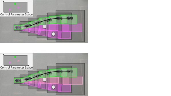
To address the limitations of existing approaches, this paper proposes a real-time, receding-horizon motion planning algorithm named REchability-based trajectory design using robust Feedback lInearization and zoNotopEs (REFINE) depicted in Figure 1 that builds on the reachability-based approach developed in [13] by using feedback linearization and zonotopes. This papers contributions are three-fold: First, a novel parameterized robust controller that partially linearizes the vehicle dynamics even in the presence of modeling error. Second, a method to perform zonotope-based reachability analysis on a closed-loop, full-order vehicle dynamics to compute a control-parameterized, over-approximate Forward Reachable Sets (FRS) that describes the vehicle behavior. Because reachability analysis is applied to the full-order model, potential conservativeness introduced by using a simplified model is avoided. Finally, an online planning framework that performs control synthesis in a receding horizon fashion by solving optimization problems in which the offline computed FRS approximation is used to check against collisions. This control synthesis framework applies to All-Wheel, Front-Wheel, or Rear-Wheel-Drive vehicle models.

The rest of this manuscript is organized as follows: Section II describes necessary preliminaries and Section III describes the dynamics of Front-Wheel-Drive vehicles. Section IV explains the trajectory design and vehicle safety in considered dynamic environments. Section V formulates the robust partial feedback linearization controller. Section VI describes Reachability-based Trajectory Design and how to perform offline reachability analysis using zonotopes. Section VII formulates the online planning using an optimization program, and in Section VIII the proposed method is extended to various perspectives including All-Wheel-Drive and Rear-Wheel-Drive vehicle models. Section IX describes how the proposed method is evaluated and compared to other state of the art methods in simulation and in hardware demo on a 1/10th race car model. And Section X concludes the paper.

II Preliminaries

This section defines notations and set representations that are used throughout the remainder of this manuscript. Sets and subspaces are typeset using calligraphic font. Subscripts are primarily used as an index or to describe an particular coordinate of a vector.

Let $\mathbb{R}$ , $\mathbb{R}_{+}$ and $\mathbb{N}$ denote the spaces of real numbers, real positive numbers, and natural numbers, respectively. Let $0_{n_{1}\times n_{2}}$ denote the $n_{1}$ -by- $n_{2}$ zero matrix. The Minkowski sum between two sets $\mathcal{A}$ and $\mathcal{A}^{\prime}$ is $\mathcal{A}\oplus\mathcal{A}^{\prime}=\{a+a^{\prime}\mid a\in\mathcal{A},~{}a^{\prime}\in\mathcal{A}^{\prime}\}$ . The power set of a set $\mathcal{A}$ is denoted by $P(\mathcal{A})$ . Given vectors $\alpha,\beta\in\mathbb{R}^{n}$ , let $[\alpha]_{i}$ denote the $i$ -th element of $\alpha$ , let $\texttt{sum}(\alpha)$ denote the summation of all elements of $\alpha$ , let $\|\alpha\|$ denote the Euclidean norm of $\alpha$ , let $\texttt{diag}(\alpha)$ denote the diagonal matrix with $\alpha$ on the diagonal, and let $\texttt{int}(\alpha,\beta)$ denote the $n$ -dimensional box $\{\gamma\in\mathbb{R}^{n}\mid[\alpha]_{i}\leq[\gamma]_{i}\leq[\beta]_{i},~{}\forall i=1,\ldots,n\}$ . Given $\alpha\in\mathbb{R}^{n}$ and $\epsilon>0$ , let $\mathcal{B}(\alpha,\epsilon)$ denote the $n$ -dimensional closed ball with center $\alpha$ and radius $\epsilon$ under the Euclidean norm. Given arbitrary matrix $A\in\mathbb{R}^{n_{1}\times n_{2}}$ , let $A^{\top}$ be the transpose of $A$ , let $[A]_{i:}$ and $[A]_{:i}$ denote the $i$ -th row and column of $A$ for any $i$ respectively, and let $|A|$ be the matrix computed by taking the absolute value of every element in $A$ .

Next, we introduce a subclass of polytopes, called zonotopes, that are used throughout this paper:

Definition 1.

A zonotope $\mathcal{Z}$ is a subset of $\mathbb{R}^{n}$ defined as

\mathcal{Z}=\left\{x\in\mathbb{R}^{n}\mid x=c+\sum_{k=1}^{\ell}\beta_{k}g_{k},\quad\beta_{k}\in[-1,1]\right\}

(1)

with center $c\in\mathbb{R}^{n}$ and $\ell$ generators $g_{1},\ldots,g_{\ell}\in\mathbb{R}^{n}$ . For convenience, we denote $\mathcal{Z}$ as $\text{\textless}c,\;G\text{\textgreater}$ where $G=[g_{1},g_{2},\ldots,g_{\ell}]\in\mathbb{R}^{n\times\ell}$ .

Note that an $n$ -dimensional box is a zonotope because

\texttt{int}(\alpha,\beta)=\text{\textless}\frac{1}{2}(\alpha+\beta),\;\frac{1}{2}\texttt{diag}(\beta-\alpha)\text{\textgreater}.

(2)

By definition the Minkowski sum of two arbitrary zonotopes $\mathcal{Z}_{1}=\text{\textless}c_{1},\;G_{1}\text{\textgreater}$ and $\mathcal{Z}_{2}=\text{\textless}c_{2},\;G_{2}\text{\textgreater}$ is still a zonotope as $\mathcal{Z}_{1}\oplus\mathcal{Z}_{2}=\text{\textless}c_{1}+c_{2},\;[G_{1},G_{2}]\text{\textgreater}$ . Finally, one can define the multiplication of a matrix $A$ of appropriate size with a zonotope $\mathcal{Z}=\text{\textless}c,\;G\text{\textgreater}$ as

A\mathcal{Z}=\left\{x\in\mathbb{R}^{n}\mid x=Ac+\sum_{k=1}^{\ell}\beta_{k}Ag_{k},~{}\beta_{k}\in[-1,1]\right\}.

(3)

Note in particular that $A\mathcal{Z}$ is equal to the zonotope $\text{\textless}Ac,\;AG\text{\textgreater}$ .

III Vehicle Dynamics

This section describes the vehicle models that we used in both high-speed and low-speed scenarios throughout this manuscript for autonomous navigation with safety concerns.

III-A Vehicle Model

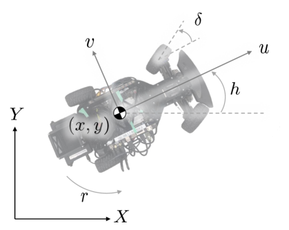
The approach described in this paper can be applied to a front-wheel-drive (FWD), rear-wheel drive (RWD), or all-wheel drive (AWD) vehicle models. However, to simplify exposition, we focus on how the approach applies to FWD vehicles and describe how to extend the approach to AWD or RWD vehicles in Section VIII-C. To simplify exposition, we attach a body-fixed coordinate frame in the horizontal plane to the vehicle as shown in Fig. 2. This body frame’s origin is the center of mass of the vehicle, and its axes are aligned with the longitudinal and lateral directions of the vehicle. Let $z^{\text{hi}}(t)=[x(t),y(t),h(t),u(t),v(t),r(t)]^{\top}\in\mathbb{R}^{6}$ be the states of the vehicle model at time $t$ , where $x(t)$ and $y(t)$ are the position of vehicle’s center of mass in the world frame, $h(t)$ is the heading of the vehicle in the world frame, $u(t)$ and $v(t)$ are the longitudinal and lateral speeds of the vehicle in its body frame, $r(t)$ is the yaw rate of the vehicle center of mass, and $\delta(t)$ is the steering angle of the front tire. To simplify exposition, we assume vehicle weight is uniformly distributed and ignore the aerodynamic effect while modeling the flat ground motion of the vehicles by the following dynamics [19, Chapter 10.4]:

\dot{z}^{\text{hi}}(t)=\begin{bmatrix}\dot{x}(t)\\ \dot{y}(t)\\ \dot{h}(t)\\ \dot{u}(t)\\ \dot{v}(t)\\ \dot{r}(t)\end{bmatrix}=\begin{bmatrix}u(t)\cos h(t)-v(t)\sin h(t)\\ u(t)\sin h(t)+v(t)\cos h(t)\\ r(t)\\ \frac{1}{m}\big{(}F_{\text{xf}}(t)+F_{\text{xr}}(t)\big{)}+v(t)r(t)\\ \frac{1}{m}\big{(}F_{\text{yf}}(t)+F_{\text{yr}}(t)\big{)}-u(t)r(t)\\ \frac{1}{I_{\text{zz}}}\big{(}l_{\text{f}}F_{\text{yf}}(t)-l_{\text{r}}F_{\text{yr}}(t)\big{)}\end{bmatrix}

(4)

where $l_{\text{f}}$ and $l_{\text{r}}$ are the distances from center of mass to the front and back of the vehicle, $I_{\text{zz}}$ is the vehicle’s moment of inertia, and $m$ is the vehicle’s mass. Note: $l_{\text{f}}$ , $l_{\text{r}}$ , $I_{\text{zz}}$ and $m$ are all constants and are assumed to be known. The tire forces along the longitudinal and lateral directions of the vehicle at time $t$ are $F_{\text{xi}}(t)$ and $F_{\text{yi}}(t)$ respectively, where the ‘i’ subscript can be replaced by ‘f’ for the front wheels or ‘r’ for the rear wheels.

To describe the tire forces along the longitudinal and lateral directions, we first define the wheel slip ratio as

\lambda_{\text{i}}(t)=\begin{dcases}\frac{r_{\text{w}}\omega_{\text{i}}(t)-u(t)}{u(t)}~{}\quad\text{during braking}\\ \frac{r_{\text{w}}\omega_{\text{i}}(t)-u(t)}{r_{\text{w}}\omega_{\text{i}}(t)}~{}\quad\text{during acceleration}\end{dcases}

(5)

where the ‘i’ subscript can be replaced as described above by ’f’ for the front wheels or ’r’ for the rear wheels, $r_{\text{w}}$ is the wheel radius, $\omega_{\text{i}}(t)$ is the tire-rotational speed at time $t$ , braking corresponds to whenever $r_{\text{w}}\omega_{\text{i}}(t)-u(t)<0$ , and acceleration corresponds to whenever $r_{\text{w}}\omega_{\text{i}}(t)-u(t)\geq 0$ . Then the longitudinal tire forces [20, Chapter 4] are computed as

	$\displaystyle F_{\text{xf}}(t)$	$\displaystyle=\frac{mgl_{\text{r}}}{l}\mu(\lambda_{\text{f}}(t)),$		(6)
	$\displaystyle F_{\text{xr}}(t)$	$\displaystyle=\frac{mgl_{\text{f}}}{l}\mu(\lambda_{\text{r}}(t)),$		(7)

where $g$ is the gravitational acceleration constant, $l=l_{\text{f}}+l_{\text{r}}$ , and $\mu(\lambda_{\text{i}}(t))$ gives the surface-adhesion coefficient and is a function of the surface being driven on [20, Chapter 13.1]. Note that in FWD vehicles, the longitudinal rear wheel tire force has a much simpler expression:

Remark 2 ([19]).

In a FWD vehicle, $F_{\text{xr}}(t)=0$ for all $t$ .

For the lateral direction, define slip angles of front and rear tires as

	$\displaystyle\alpha_{\text{f}}(t)$	$\displaystyle=\delta(t)-\frac{v(t)+l_{\text{f}}r(t)}{u(t)},$		(8)
	$\displaystyle\alpha_{\text{r}}(t)$	$\displaystyle=-\frac{v(t)-l_{\text{r}}r(t)}{u(t)},$		(9)

then the lateral tire forces [20, Chapter 4] are real-valued functions of the slip angles:

	$\displaystyle F_{\text{yf}}(t)$	$\displaystyle=c_{\alpha\text{f}}(\alpha_{\text{f}}(t)),$		(10)
	$\displaystyle F_{\text{yr}}(t)$	$\displaystyle=c_{\alpha\text{r}}(\alpha_{\text{r}}(t)).$		(11)

Note $\mu,~{}c_{\alpha\text{f}}$ and $c_{\alpha\text{r}}$ are all nonlinear functions, but share similar characteristics. In particular, they behave linearly when the slip ratio and slip angle are close to zero, but saturate when the magnitudes of the slip ratio and slip angle reach some critical values of $\lambda^{\text{cri}}$ and $\alpha^{\text{cri}}$ , respectively, then decrease slowly [20, Chapter 4, Chapter 13]. As we describe in Section VIII-B, during trajectory optimization we are able to guarantee that $\mu,~{}c_{\alpha\text{f}}$ and $c_{\alpha\text{r}}$ operate in the linear regime. As a result, to simplify exposition until we reach Section VIII-B, we make the following assumption:

Assumption 3.

The absolute values of the the slip ratio and angle are bounded below their critical values (i.e., $|\lambda_{\text{f}}(t)|,|\lambda_{\text{r}}(t)|<\lambda^{\text{cri}}$ and $|\alpha_{\text{f}}(t)|,|\alpha_{\text{r}}(t)|<\alpha^{\text{cri}}$ hold for all time).

Assumption 3 ensures that the longitudinal tire forces can be described as

	$\displaystyle F_{\text{xf}}(t)$	$\displaystyle=\frac{mgl_{\text{r}}}{l}\bar{\mu}\lambda_{\text{f}}(t),$		(12)
	$\displaystyle F_{\text{xr}}(t)$	$\displaystyle=\frac{mgl_{\text{f}}}{l}\bar{\mu}\lambda_{\text{r}}(t),$		(12)

and the lateral tire forces can be described as

	$\displaystyle F_{\text{yf}}(t)$	$\displaystyle=\bar{c}_{\alpha\text{f}}\alpha_{\text{f}}(t),$		(13)
	$\displaystyle F_{\text{yr}}(t)$	$\displaystyle=\bar{c}_{\alpha\text{r}}\alpha_{\text{r}}(t),$		(13)

with constants $\bar{\mu},\bar{c}_{\alpha\text{f}},\bar{c}_{\alpha\text{r}}\in\mathbb{R}$ . Note $\bar{c}_{\alpha\text{f}}$ and $\bar{c}_{\alpha\text{r}}$ are referred to as cornering stiffnesses.

Note that the steering angle of the front wheel, $\delta$ , and the tire rotational speed, $\omega_{\text{i}}$ , are the inputs that one is able to control. In particular for an AWD vehicle, both $\omega_{\text{f}}$ and $\omega_{\text{r}}$ are inputs; whereas, in a FWD vehicle only $\omega_{\text{f}}$ is an input. When we formulate our controller in Section V for a FWD vehicle we begin by assuming that we can directly control the front tire forces, $F_{\text{xf}}$ and $F_{\text{yf}}$ . We then illustrate how to compute $\delta$ and $\omega_{\text{f}}$ when given $F_{\text{xf}}$ and $F_{\text{yf}}$ . For an AWD vehicle, we describe in Section VIII-C, how to compute $\delta$ , $\omega_{\text{f}}$ , and $\omega_{\text{r}}$ .

In fact, as we describe in Section V, our approach to perform control relies upon estimating the rear tire forces and controlling the front tire forces by applying appropriate tire speed and steering angle. Unfortunately, in the real-world our state estimation and models for front and rear tire forces may be inaccurate and aerodynamic-drag force could also affect vehicle dynamics [20, Section 4.2]. To account for the inaccuracy, we extend the vehicle dynamic model in (4) by introducing a time-varying affine modeling error $\Delta_{u},\Delta_{v},\Delta_{r}$ into the dynamics of $u,v,$ and $r$ :

\displaystyle\dot{z}^{\text{hi}}(t)

\displaystyle=\begin{bmatrix}u(t)\cos h(t)-v(t)\sin h(t)\\ u(t)\sin h(t)+v(t)\cos h(t)\\ r(t)\\ \frac{1}{m}\big{(}F_{\text{xf}}(t)+F_{\text{xr}}(t)\big{)}+v(t)r(t)+\Delta_{u}(t)\\ \frac{1}{m}\big{(}F_{\text{yf}}(t)+F_{\text{yr}}(t)\big{)}-u(t)r(t)+\Delta_{v}(t)\\ \frac{1}{I_{\text{zz}}}\big{(}l_{\text{f}}F_{\text{yf}}(t)-l_{\text{r}}F_{\text{yr}}(t)\big{)}+\Delta_{r}(t)\end{bmatrix}.

(14)

Note, we have abused notation and redefined $\dot{z}^{\text{hi}}$ which was originally defined in (4). For the remainder of this paper, we assume that the dynamics $\dot{z}^{\text{hi}}$ evolves according to (14). To ensure that this definition is well-posed (i.e. their solution exists and is unique) and to aid in the development of our controller as described in Section V, we make the following assumption:

Assumption 4.

$\Delta_{u},\Delta_{v},\Delta_{r}$ are all square integrable functions and are bounded (i.e., there exist real numbers $M_{u},M_{v},M_{r}\in[0,+\infty)$ such that $\|\Delta_{u}(t)\|_{\infty}\leq M_{u},~{}\|\Delta_{v}(t)\|_{\infty}\leq M_{v},~{}\|\Delta_{r}(t)\|_{\infty}\leq M_{r}$ for all $t$ ).

Note in Section IX-C1, we explain how to compute $\Delta_{u},\Delta_{v},\Delta_{r}$ using real-world data.

III-B Low-Speed Vehicle Model

When the vehicle speed lowers below some critical value $u^{\text{cri}}>0$ , the denominator of the wheel slip ratio (5) and tire slip angles (8) and (9) approach zero which makes applying the model described in (4) intractable. As a result, in this work when $u(t)\leq u^{\text{cri}}$ the dynamics of a vehicle are modeled using a steady-state cornering model [21, Chapter 6], [22, Chapter 5], [23, Chapter 10]. Note that the critical velocity $u^{\text{cri}}$ can be found according to [24, (5) and (18)].

The steady-state cornering model or low-speed vehicle model is described using four states, $z^{\text{lo}}(t)=[x(t),y(t),h(t),u(t)]^{\top}\in\mathbb{R}^{4}$ at time $t$ . This model ignores transients on lateral velocity and yaw rate. Note that the dynamics of $x$ , $y$ , $h$ and $u$ are the same as in the high speed model (14); however, the steady-state corning model describes the yaw rate and lateral speed as

	$\displaystyle v^{\text{lo}}(t)=$	$\displaystyle l_{\text{r}}r^{\text{lo}}(t)-\frac{ml_{\text{f}}}{\bar{c}_{\alpha\text{r}}l}u(t)^{2}r^{\text{lo}}(t)$		(15)
	$\displaystyle r^{\text{lo}}(t)=$	$\displaystyle\frac{\delta(t)u(t)}{l+C_{\text{us}}u(t)^{2}}$		(16)

with understeer coefficient

C_{\text{us}}=\frac{m}{l}\left(\frac{l_{\text{r}}}{\bar{c}_{\alpha\text{f}}}-\frac{l_{\text{f}}}{\bar{c}_{\alpha\text{r}}}\right).

(17)

As a result, $\dot{z}^{\text{lo}}$ satisfies the dynamics of the first four states in (4) except with $r^{\text{lo}}$ taking the role of $r$ and $v^{\text{lo}}$ taking the role of $v$ .

Notice when $u(t)=v(t)=r(t)=0$ and the longitudinal tire forces are zero, $\dot{u}(t)$ could still be nonzero due to a nonzero $\Delta_{u}(t)$ . To avoid this issue, we make a tighter assumption on $\Delta_{u}(t)$ without violating Assumption 4:

Assumption 5.

For all $t$ such that $u(t)\in[0,u^{\text{cri}}]$ , $|\Delta_{u}(t)|$ is bounded from above by a linear function of $u(t)$ (i.e.,

|\Delta_{u}(t)|\leq b_{u}^{\text{pro}}\cdot u(t)+b_{u}^{\text{off}},\text{ if }u(t)\in[0,u^{\text{cri}}],

(18)

where $b_{u}^{\text{pro}}$ and $b_{u}^{\text{off}}$ are constants satisfying $b_{u}^{\text{pro}}\cdot u^{\text{cri}}+b_{u}^{\text{off}}\leq M_{u}$ ). In addition, $\Delta_{u}(t)=0$ if $u(t)=0$ .

As we describe in detail in Section V-C, the high-speed and low-speed models can be combined together as a hybrid system to describe the behavior of the vehicle across all longitudinal speeds. In short, when $u$ transitions past the critical speed $u^{\text{cri}}$ from above at time $t$ , the low speed model’s states are initialized as:

z^{\text{lo}}(t)=\pi_{1:4}(z^{\text{hi}}(t))

(19)

where $\pi_{1:4}:\mathbb{R}^{6}\rightarrow\mathbb{R}^{4}$ is the projection operator that projects $z^{\text{hi}}(t)$ onto its first four dimensions via the identity relation. If $u$ transitions past the critical speed from below at time $t$ , the high speed model’s states are initialized as

z^{\text{hi}}(t)=[z^{\text{lo}}(t)^{\top},v^{\text{lo}}(t),r^{\text{lo}}(t)]^{\top}.

(20)

IV Trajectory Design and Safety

This section describes the space of trajectories that are optimized over at run-time within REFINE, how this paper defines safety during motion planning via the notion of not-at-fault behavior, and what assumptions this paper makes about the environment surrounding the ego-vehicle.

IV-A Trajectory Parameterization

Each trajectory plan is specified over a compact time interval. Without loss of generality, we let this compact time interval have a fixed duration $t_{\text{f}}$ . Because REFINE performs receding-horizon planning, we make the following assumption about the time available to construct a new plan:

Assumption 6.

During each planning iteration starting from time $t_{0}$ , the ego vehicle has $t_{\text{plan}}$ seconds to find a control input. This control input is applied during the time interval $[t_{0}+t_{\text{plan}},t_{0}+t_{\text{plan}}+t_{\text{f}}]$ where $t_{\text{f}}\geq 0$ is a user-specified constant. In addition, the state of the vehicle at time $t_{0}+t_{\text{plan}}$ is known at time $t_{0}$ .

In each planning iteration, REFINE chooses a trajectory to be followed by the ego vehicle. These trajectories are chosen from a pre-specified continuum of trajectories, with each uniquely determined by a trajectory parameter $p\in\mathcal{P}$ . Let $\mathcal{P}\subset\mathbb{R}^{n_{p}}$ , $n_{p}\in\mathbb{N}$ be a n-dimensional box $\texttt{int}(\underline{p},\overline{p})$ where $\underline{p},\overline{p}\in\mathbb{R}^{n_{p}}$ indicate the element-wise lower and upper bounds of $p$ , respectively. We define these desired trajectories as follows:

Definition 7.

For each $p\in\mathcal{P}$ , a desired trajectory is a function for the longitudinal speed, $u^{\text{des}}(\cdot,p):[t_{0}+t_{\text{plan}},t_{\text{f}}]\to\mathbb{R}$ , a function for the heading, $h^{\text{des}}(\cdot,p):[t_{0}+t_{\text{plan}},t_{\text{f}}]\to\mathbb{R}$ , and a function for the yaw rate, $r^{\text{des}}(\cdot,p):[t_{0}+t_{\text{plan}},t_{\text{f}}]\to\mathbb{R}$ , that satisfy the following properties.

1.

For all $p\in\mathcal{P}$ , there exists a time instant $t_{\text{m}}\in[t_{0}+t_{\text{plan}},t_{\text{f}})$ after which the desired trajectory begins to brake (i.e., $|u^{\text{des}}(t,p)|$ , $|h^{\text{des}}(t,p)|$ and $|r^{\text{des}}(t,p)|$ are non-increasing for all $t\in[t_{\text{m}},t_{\text{f}}]$ ).
2.

The desired trajectory eventually comes to and remains stopped (i.e., there exists a $t_{\text{stop}}\in[t_{0}+t_{\text{plan}},t_{\text{f}}]$ such that $u^{\text{des}}(t,p)=h^{\text{des}}(t,p)=r^{\text{des}}(t,p)=0$ for all $t\geq t_{\text{stop}}$ ).
3.

$u^{\text{des}}$ and $h^{\text{des}}$ are piecewise continuously differentiable [25, Chapter 6, $\S$ 1.1] with respect to $t$ and $p$ .
4.

The time derivative of the heading function is equal to the yaw rate function (i.e., $r^{\text{des}}(t,p)=\frac{\partial}{\partial t}h^{\text{des}}(t,p)$ over all regions that $h^{\text{des}}(t,p)$ is continuously differentiable with respect to $t$ ).

The first two properties ensure that a fail safe contingency braking maneuver is always available and the latter two properties ensure that the tracking controller described in Section V is well-defined. Note that sometimes we abuse notation and evaluate a desired trajectory for $t>t_{\text{f}}$ . In this instance, the value of the desired trajectory is equal to its value at $t_{\text{f}}$ .

IV-B Not-At-Fault

In dynamic environments, avoiding collision may not always be possible (e.g. a parked car can be run into). As a result, we instead develop a trajectory synthesis technique which ensures that the ego vehicle is not-at-fault [26]:

Definition 8.

The ego vehicle is not-at-fault if it is stopped, or if it is never in collision with any obstacles while it is moving.

In other words, the ego vehicle is not responsible for a collision if it has stopped and another vehicle collides with it. One could use a variant of not-at-fault and require that when the ego-vehicle comes to a stop it leave enough time for all surrounding vehicles to come safely to a stop as well. The remainder of the paper can be generalized to accommodate this variant of not-at-fault; however, in the interest of simplicity we use the aforementioned definition.

Remark 9.

Under Assumption 3, neither longitudinal nor lateral tire forces saturate (i.e., drifting cannot occur). As a result, if the ego vehicle has zero longitudinal speed, it also has zero lateral speed and yaw rate. Therefore in Definition 8, the ego vehicle being stopped is equivalent to its longitudinal speed being $0$ .

IV-C Environment and Sensing

To provide guarantees about vehicle behavior in a receding horizon planning framework and inspired by [15, Section 3], we define the ego vehicle’s footprint as:

Definition 10.

Given $\mathcal{W}\subset\mathbb{R}^{2}$ as the world space, the ego vehicle is a rigid body that lies in a rectangular $\mathcal{O}^{\text{ego}}:=\texttt{int}([-0.5L,-0.5W]^{T},[0.5L,0.5W]^{T})\subset\mathcal{W}$ with width $W>0$ , length $L>0$ at time $t=0$ . Such $\mathcal{O}^{\text{ego}}$ is called the footprint of the ego vehicle.

In addition, we define the dynamic environment in which the ego vehicle is operating within as:

Definition 11.

An obstacle is a set $\mathcal{O}_{i}(t)\subset\mathcal{W}$ that the ego vehicle cannot intersect with at time $t$ , where $i\in\mathcal{I}$ is the index of the obstacle and $\mathcal{I}$ contains finitely many elements.

The dependency on $t$ in the definition of an obstacle allows the obstacle to move as $t$ varies. However if the $i$ -th obstacle is static, then $\mathcal{O}_{i}(t)$ remains constant at all time. Assuming that the ego vehicle has a maximum speed $\nu^{\text{ego}}$ and all obstacles have a maximum speed $\nu^{\text{obs}}$ for all time, we then make the following assumption on planning and sensing horizon.

Assumption 12.

The ego vehicle senses all obstacles within a sensor radius $S>(t_{\text{f}}+t_{\text{plan}})\cdot(\nu^{\text{ego}}+\nu^{\text{obs}})+0.5\sqrt{L^{2}+W^{2}}$ around its center of mass.

Assumption 12 ensures that any obstacle that can cause a collision between times $t\in[t_{0}+t_{\text{plan}},t_{0}+t_{\text{plan}}+t_{\text{f}}]$ can be detected by the vehicle [15, Theorem 15]. Note one could treat sensor occlusions as a obstacles that travel at the maximum obstacle speed [27, 28].

V Controller Design and Hybrid System Model

This section describes the control inputs that we use to follow the desired trajectories and describes the closed-loop hybrid system vehicle model. Recall that the control inputs to the vehicle dynamics model are the steering angle of the front wheel, $\delta$ , and the tire rotational speed, $\omega_{\text{i}}$ . Section V-A describes how to select front tire forces to follow a desired trajectory and Section V-B describes how to compute a steering angle and tire rotational speed input from these computed front tire forces. Section V-C describes the closed-loop hybrid system model of the vehicle under the chosen control input. Note that this section focuses on the FWD vehicle model.

V-A Robust Controller

Because applying reachability analysis to linear systems generates tighter approximations of the system behavior when compared to nonlinear systems, we propose to develop a feedback controller that linearizes the dynamics. Unfortunately, because both the high-speed and low-speed models introduced in Section III are under-actuated (i.e., the dimension of control inputs is smaller than that of system state), our controller is only able to partially feedback linearize the vehicle dynamics. Such controller is also expected to be robust such that it can account for computational errors as described in Assumptions 4 and 5.

We start by introducing the controller on longitudinal speed whose dynamics appears in both high-speed and low-speed models. Recall $\|\Delta_{u}(t)\|_{\infty}\leq M_{u}$ in Assumption 4. Inspired by the controller developed in [29], we set the longitudinal front tire force to be

\begin{split}F_{\text{xf}}(t)=-mK_{u}(u(t)-u^{\text{des}}(t,p))+m\dot{u}^{\text{des}}(t,p)+\\ -F_{\text{xr}}(t)-mv(t)r(t)+m\tau_{u}(t,p),\end{split}

(21)

where

$\displaystyle\tau_{u}(t,p)=$	$\displaystyle-\big{(}\kappa_{u}(t,p)M_{u}+\phi_{u}(t,p)\big{)}e_{u}(t,p),$	(22)
$\displaystyle\kappa_{u}(t,p)=$	$\displaystyle\kappa_{1,u}+\kappa_{2,u}\int_{t_{0}}^{t}\\|u(s)-u^{\text{des}}(s,p)\\|^{2}ds,$	(23)
$\displaystyle\phi_{u}(t,p)=$	$\displaystyle\phi_{1,u}+\phi_{2,u}\int_{t_{0}}^{t}\\|u(s)-u^{\text{des}}(s,p)\\|^{2}ds,$	(24)
$\displaystyle e_{u}(t,p)=$	$\displaystyle u(t)-u^{\text{des}}(t,p),$	(25)

with user-chosen constants $\kappa_{1,u},\kappa_{2,u},\phi_{1,u},\phi_{2,u}\in\mathbb{R}_{+}$ . Note in (21) we have suppressed the dependence on $p$ in $F_{\text{xf}}(t)$ for notational convenience. Using (21), the closed-loop dynamics of $u$ become:

\begin{split}\dot{u}(t)=\tau_{u}(t,p)+\Delta_{u}(t)+\dot{u}^{\text{des}}(t,p)+\\ -K_{u}\left(u(t)-u^{\text{des}}(t,p)\right).\end{split}

(26)

The same control strategy can be applied to vehicle yaw rate whose dynamics only appear in the high-speed vehicle model. Let the lateral front tire force be

\begin{split}F_{\text{yf}}(t)=-\frac{I_{\text{zz}}K_{r}}{l_{\text{f}}}\left(r(t)-r^{\text{des}}(t,p)\right)+\frac{I_{\text{zz}}}{l_{\text{f}}}\dot{r}^{\text{des}}(t,p)+\\ -\frac{I_{\text{zz}}K_{h}}{l_{\text{f}}}\left(h(t)-h^{\text{des}}(t,p)\right)+\frac{l_{\text{r}}}{l_{\text{f}}}F_{\text{yr}}(t)+\frac{I_{\text{zz}}}{l_{\text{f}}}\tau_{r}(t,p),\end{split}

(27)

where

$\displaystyle\tau_{r}(t,p)=$	$\displaystyle-\big{(}\kappa_{r}(t,p)M_{r}+\phi_{r}(t,p)\big{)}e_{r}(t,p)$	(28)
$\displaystyle\kappa_{r}(t,p)=$	$\displaystyle\kappa_{1,r}+\kappa_{2,r}\int_{t_{0}}^{t}\left\\|\begin{bmatrix}r(s)\\ h(s)\end{bmatrix}-\begin{bmatrix}r^{\text{des}}(s,p)\\ h^{\text{des}}(s,p)\end{bmatrix}\right\\|^{2}ds$	(29)
$\displaystyle\phi_{r}(t,p)=$	$\displaystyle\phi_{1,r}+\phi_{2,r}\int_{t_{0}}^{t}\left\\|\begin{bmatrix}r(s)\\ h(s)\end{bmatrix}-\begin{bmatrix}r^{\text{des}}(s,p)\\ h^{\text{des}}(s,p)\end{bmatrix}\right\\|^{2}ds$	(30)
$\displaystyle e_{r}(t,p)=$	$\displaystyle\begin{bmatrix}K_{r}&K_{h}\end{bmatrix}\begin{bmatrix}r(t)-r^{\text{des}}(t,p)\\ h(t)-h^{\text{des}}(t,p)\end{bmatrix}$	(31)

with user-chosen constants $\kappa_{1,r},\kappa_{2,r},\phi_{1,r},\phi_{2,r}\in\mathbb{R}_{+}$ . Note in (27) we have again suppressed the dependence on $p$ in $F_{\text{yf}}(t)$ for notational convenience. Using (27), the closed-loop dynamics of $r$ become:

\begin{split}\dot{r}(t)=&\tau_{r}(t,p)+\Delta_{r}(t)+\dot{r}^{\text{des}}(t,p)+\\ &-K_{r}\big{(}r(t)-r^{\text{des}}(t,p)\big{)}+\\ &-K_{h}\big{(}h(t)-h^{\text{des}}(t,p)\big{)}.\end{split}

(32)

Using (27), the closed-loop dynamics of $v$ become:

\begin{split}\dot{v}(t)=\frac{1}{m}\Bigg{(}\frac{l}{l_{\text{f}}}F_{\text{yr}}(t)+\frac{I_{\text{zz}}}{l_{\text{f}}}\Big{(}\tau_{r}(t,p)+\dot{r}^{\text{des}}(t,p)+\\ -u(t)r(t)+\Delta_{v}(t)-K_{r}\big{(}r(t)-r^{\text{des}}(t,p)\big{)}+\\ -K_{h}\big{(}h(t)-h^{\text{des}}(t,p)\big{)}\Big{)}\Bigg{)}.\end{split}

(33)

Because $u^{\text{des}}$ , $r^{\text{des}}$ , and $h^{\text{des}}$ depend on trajectory parameter $p$ , one can rewrite the closed loop high-speed and low-speed vehicle models as

	$\displaystyle\dot{z}^{\text{hi}}(t)$	$\displaystyle=f^{\text{hi}}(t,z^{\text{hi}}(t),p),$		(34)
	$\displaystyle\dot{z}^{\text{lo}}(t)$	$\displaystyle=f^{\text{lo}}(t,z^{\text{lo}}(t),p),$		(35)

where dynamics of $x$ , $y$ and $h$ are stated as the first three dimensions in (4), closed-loop dynamics of $u$ is described in (26), and closed-loop dynamics of $v$ and $r$ in the high-speed model are presented in (33) and (32). Note that the lateral tire force could be defined to simplify the dynamics on $v$ instead of $r$ , but the resulting closed loop system may differ. Controlling the yaw rate may be easier in real applications, because $r$ can be directly measured by an IMU unit.

V-B Extracting Wheel Speed and Steering Inputs

Because we are unable to directly control tire forces, it is vital to compute wheel speed and steering angle such that the proposed controller described in (21) and (27) is viable. Under Assumption 3, wheel speed and steering inputs can be directly computed in closed form. The wheel speed to realize longitudinal front tire force (21) can be derived from (5) and (12) as

\omega_{\text{f}}(t)=\begin{dcases}\left(\frac{lF_{\text{xf}}(t)}{\bar{\mu}mgl_{\text{r}}}+1\right)\frac{u(t)}{r_{\text{w}}}~{}\quad\text{during braking},\\ \frac{u(t)}{\left(1-\frac{lF_{\text{xf}}(t)}{\bar{\mu}mgl_{\text{r}}}\right)r_{\text{w}}}\hskip 29.87547pt\text{during acceleration}.\end{dcases}

(36)

Similarly according to (8) and (13), the steering input

\delta(t)=\frac{F_{\text{yf}}(t)}{\bar{c}_{\alpha\text{f}}}+\frac{v(t)+l_{\text{f}}r(t)}{u(t)}

(37)

achieves the lateral front tire force in (27) when $u(t)>u^{\text{cri}}$ .

Notice lateral tire forces does not appear in the low-speed dynamics, but one is still able to control the lateral behavior of the ego vehicle. Based on (15) and (16), yaw rate during low-speed motion is directly controlled by steering input $\delta(t)$ and lateral velocity depends on yaw rate. Thus to achieve desired behavior on the lateral direction, one can set the steering input to be

\delta(t)=\frac{r^{\text{des}}(t)(l+C_{\text{us}}u(t)^{2})}{u(t)}.

(38)

V-C Augmented State and Hybrid Vehicle Model

To simplify the presentation throughout the remainder of the paper, we define a hybrid system model of the vehicle dynamics that switches between the high and low speed vehicle models when passing through the critical longitudinal velocity. In addition, for computational reasons that are described in subsequent sections, we augment the initial condition of the system to the state vector while describing the vehicle dynamics. In particular, denote $z_{0}=[(z^{\text{pos}}_{0})^{\top},(z^{\text{vel}}_{0})^{\top}]^{\top}\in\mathcal{Z}_{0}\subset\mathbb{R}^{6}$ the initial condition of the ego vehicle where $z^{\text{pos}}_{0}=[x_{0},y_{0},h_{0}]^{\top}\in\mathbb{R}^{3}$ gives the value of $[x(t),y(t),h(t)]^{\top}$ and $z^{\text{vel}}_{0}=[u_{0},v_{0},r_{0}]^{\top}\in\mathbb{R}^{3}$ gives the value of $[u(t),v(t),r(t)]^{\top}$ at time $t=0$ . Then we augment the initial velocity condition $z^{\text{vel}}_{0}\in\mathbb{R}^{3}$ of the vehicle model and trajectory parameter $p$ into the vehicle state vector as $z^{\text{aug}}(t)=[x(t),y(t),h(t),u(t),v(t),r(t),(z^{\text{vel}}_{0})^{\top},p^{\top}]^{\top}\in\mathbb{R}^{9}\times\mathcal{P}\subset\mathbb{R}^{9+n_{p}}$ . Note the last $3+n_{p}$ states are static with respect to time. As a result, the dynamics of the augmented vehicle state during high-speed and low-speed scenarios can be written as

\dot{z}^{\text{aug}}(t)=\begin{dcases}\begin{bmatrix}f^{\text{hi}}(t,z^{\text{hi}}(t),p)\\ 0_{(3+n_{p})\times 1}\end{bmatrix},\text{ if }u(t)>u^{\text{cri}},\\ \\ \begin{bmatrix}f^{\text{lo}}(t,z^{\text{lo}}(t),p)\\ 0_{(5+n_{p})\times 1}\end{bmatrix},\text{ if }u(t)\leq u^{\text{cri}},\end{dcases}

(39)

which we refer to as the hybrid vehicle dynamics model. Notice when $u(t)\leq u^{\text{cri}}$ , assigning zero dynamics to $v$ and $r$ in (39) does not affect the evolution of the vehicle’s dynamics because the lateral speed and yaw rate are directly computed via longitudinal speed as in (15) and (16).

Because the vehicle’s dynamics changes depending on $u$ , it is natural to model the ego vehicle as a hybrid system $HS$ [30, Section 1.2]. The hybrid system has $z^{\text{aug}}$ as its state and consists of a high-speed mode and a low-speed mode with dynamics in (39). Instantaneous transition between the high and low speed models within $HS$ are described using the notion of a guard and reset map. The guard triggers a transition and is defined as $\{z^{\text{aug}}(t)\in\mathbb{R}^{9}\times\mathcal{P}\mid u(t)=u^{\text{cri}}\}$ . Once a transition happens, the reset map maintains the last $3+n_{p}$ dimensions of $z^{\text{aug}}(t)$ , but resets the first $6$ dimensions of $z^{\text{aug}}(t)$ via (19) if $u(t)$ approaches $u^{\text{cri}}$ from above and via (20) if $u(t)$ approaches $u^{\text{cri}}$ from below.

We next prove that for desired trajectory defined as in Definition 7 under the controllers defined in Section V, the vehicle model eventually comes to a stop. To begin note that experimentally, we observed that the vehicle quickly comes to a stop during braking once its longitudinal speed becomes $u(t)\leq 0.15$ [m/s]. Thus we make the following assumption:

Assumption 13.

Suppose $u(t)=0.15$ for some $t\geq t_{\text{stop}}$ . Then under the control inputs (21) and (27) and while tracking any desired trajectory as in Definition 7, the ego vehicle takes at most $t_{\text{fstop}}$ seconds after $t_{\text{stop}}$ to come to a complete stop.

We use this assumption to prove that the vehicle can be brought to a stop within a specified amount of time in the following lemma whose proof can be found in Appendix A:

Lemma 14.

Let $\mathcal{Z}_{0}\subset\mathbb{R}^{6}$ be a compact subset of initial conditions for the vehicle dynamic model and $\mathcal{P}$ be a compact set of trajectory parameters. Let $\Delta_{u}(t)$ be bounded for all $t$ as in Assumptions 4 and 5 with constants $M_{u}$ , $b_{u}^{\text{pro}}$ and $b_{u}^{\text{off}}$ . Let $z^{\text{aug}}$ be a solution to the hybrid vehicle dynamics model (39) beginning from $z_{0}\in\mathcal{Z}_{0}$ under trajectory parameter $p\in\mathcal{P}$ while applying the control inputs (21) and (27) to track some desired trajectory satisfying Definition 7. Assume the desired longitudinal speed satisfies the following properties: $u^{\text{des}}(0,p)=u(0)$ , $u^{\text{des}}(t,p)$ is only discontinuous at time $t_{\text{stop}}$ , and $u^{\text{des}}(t,p)$ converges to $u^{\text{cri}}$ as $t$ converges to $t_{\text{stop}}$ from below. If $K_{u}$ , $\kappa_{1,u}$ and $\phi_{1,u}$ are chosen such that $\frac{M_{u}}{\kappa_{1,u}M_{u}+\phi_{1,u}}\in(0.15,u^{\text{cri}}]$ and $\frac{(b_{u}^{\text{off}})^{2}}{4(\kappa_{1,u}M_{u}+\phi_{1,u}-b_{u}^{\text{pro}})}<0.15^{2}K_{u}$ hold, then for all $p\in\mathcal{P}$ and $z_{0}\in\mathcal{Z}_{0}$ satisfying $u(0)>0$ , there exists $t_{\text{brake}}$ such that $u(t)=0$ for all $t\geq t_{\text{brake}}$ .

Note, the proof of Lemma 14 includes an explicit formula for $t_{\text{brake}}$ in (82). This lemma is crucial because it specifies the length of time over which we should construct FRS, so that we can verify that not-at-fault behavior can be satisfied based on Definition 8 and Remark 9.

VI Computing and Using the FRS

This section describes how REFINE operates at a high-level. It then describes the offline reachability analysis of the ego vehicle as a state-augmented hybrid system using zonotopes and illustrates how the ego vehicle’s footprint can be accounted for during reachability analysis.

REFINE conservatively approximates a control-parameterized FRS of the full-order vehicle dynamics. The FRS includes all behaviors of the ego vehicle over a finite time horizon and is mathematically defined in Section VI-A. To ensure the FRS is a tight representation, REFINE relies on the controller design described in Section V. Because this controller partially linearizes the dynamics, REFINE relies on a zonotope-based reachable set representation which behave well for nearly linear systems.

During online planning, REFINE performs control synthesis by solving optimization problems in a receding horizon fashion, where the optimization problem computes a trajectory parameter to navigate the ego vehicle to a waypoint while behaving in a not-at-fault manner. As in Assumption 6, each planning iteration in REFINE is allotted $t_{\text{plan}}>0$ to generate a plan. As depicted in Figure 3, if a particular planning iteration begins at time $t_{0}$ , its goal is to find a control policy by solving an online optimization within $t_{\text{plan}}$ seconds so that the control policy can be applied during $[t_{0}+t_{\text{plan}},t_{0}+t_{\text{plan}}+t_{\text{f}}]$ . Because any trajectory in Definition 7 brings the ego vehicle to a stop, we partition $[t_{0}+t_{\text{plan}},t_{0}+t_{\text{plan}}+t_{\text{f}}]$ into $[t_{0}+t_{\text{plan}},t_{0}+t_{\text{plan}}+t_{\text{m}})$ during which a driving maneuver is tracked and $[t_{0}+t_{\text{plan}}+t_{\text{m}},t_{0}+t_{\text{plan}}+t_{\text{f}}]$ during which a contingency braking maneuver is activated. Note $t_{\text{m}}$ is not necessarily equal to $t_{\text{stop}}$ . As a result of Lemma 14, by setting $t_{\text{f}}$ equal to $t_{\text{brake}}$ one can guarantee that the ego vehicle comes to a complete stop by $t_{\text{f}}$ .

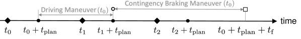
If the planning iteration at time $t_{0}$ is feasible (i.e., not-at-fault), then the entire feasible planned driving maneuver is applied during $[t_{0}+t_{\text{plan}},t_{0}+t_{\text{plan}}+t_{\text{m}})$ . If the planning iteration starting at time $t_{0}$ is infeasible, then the braking maneuver, whose safe behavior was verified in the previous planning iteration, can be applied starting at $t_{0}+t_{\text{plan}}$ to bring the ego vehicle to a stop in a not-at-fault manner. To ensure real-time performance, $t_{\text{plan}}\leq t_{\text{m}}$ . To simplify notation, we reset time to $0$ whenever a feasible control policy is about to be applied.

VI-A Offline FRS Computation

The FRS of the ego vehicle is

\begin{split}\mathcal{F}_{xy}([0,&t_{\text{f}}])=\Bigg{\{}(x,y)\in\mathcal{W}\mid\exists t\in[0,t_{\text{f}}],p\in\mathcal{P},\\ &z_{0}=\begin{bmatrix}z^{\text{pos}}_{0}\\ z^{\text{vel}}_{0}\end{bmatrix}\in\mathcal{Z}_{0}\text{ s.t. }\begin{bmatrix}x\\ y\end{bmatrix}=\pi_{xy}(z^{\text{aug}}(t)),\\ &z^{\text{aug}}\text{ is a solution of }HS\text{ with }z^{\text{aug}}(0)=\begin{bmatrix}z_{0}\\ z^{\text{vel}}_{0}\\ p\end{bmatrix}\Bigg{\}},\end{split}

(40)

where $\pi_{xy}:\mathbb{R}^{9+n_{p}}\rightarrow\mathbb{R}^{2}$ is the projection operator that outputs the first two coordinates from its argument. $\mathcal{F}_{xy}([0,t_{\text{f}}])$ collects all possible behavior of the ego vehicle while following the dynamics of $HS$ in the $xy$ -plane over time interval $[0,t_{\text{f}}]$ for all possible $p\in\mathcal{P}$ and initial condition $z_{0}\in\mathcal{Z}_{0}$ . Computing $\mathcal{F}_{xy}([0,t_{\text{f}}])$ precisely is numerically challenging because the ego vehicle is modeled as a hybrid system with nonlinear dynamics, thus we aim to compute an outer-approximation of $\mathcal{F}_{xy}([0,t_{\text{f}}])$ instead.

To outer-approximate $\mathcal{F}_{xy}([0,t_{\text{f}}])$ , we start by making the following assumption:

Assumption 15.

The initial condition space $\mathcal{Z}_{0}=\{0_{3\times 1}\}\times\mathcal{Z}^{\text{vel}}_{0}$ where $\mathcal{Z}^{\text{vel}}_{0}=\text{int}(\underline{z^{\text{vel}}_{0}},\overline{z^{\text{vel}}_{0}})\subset\mathbb{R}^{3}$ is a 3-dimensional box representing all possible initial velocity conditions $z^{\text{vel}}_{0}$ of the ego vehicle.

Because vehicles operate within a bounded range of speeds, this assumption is trivial to satisfy. Notice in particular that $\mathcal{Z}^{\text{vel}}_{0}$ is a zonotope $\text{\textless}c^{\text{vel}}_{0},\;G^{\text{vel}}_{0}\text{\textgreater}$ where $c^{\text{vel}}_{0}=\frac{1}{2}(\underline{z^{\text{vel}}_{0}}+\overline{z^{\text{vel}}_{0}})$ and $G^{\text{vel}}_{0}=\frac{1}{2}\texttt{diag}(\overline{z^{\text{vel}}_{0}}-\underline{z^{\text{vel}}_{0}})$ . We assume a zero initial position condition $z^{\text{pos}}_{0}$ in the first three dimensions of $\mathcal{Z}_{0}$ for simplicity, and nonzero $z^{\text{pos}}_{0}$ can be dealt with via coordinate transformation online as described in Section VII-A.

Recall that because $\mathcal{P}$ is a compact n-dimensional box, it can also be represented as a zonotope as $\text{\textless}c_{p},\;G_{p}\text{\textgreater}$ where $c_{p}=\frac{1}{2}(\underline{p}+\overline{p})$ and $G_{p}=\frac{1}{2}\texttt{diag}(\overline{p}-\underline{p})$ . Then the set of initial conditions for $z^{\text{aug}}(0)$ can be represented as a zonotope $\mathcal{Z}^{\text{aug}}_{0}=\text{\textless}c_{z^{\text{aug}}},\;G_{z^{\text{aug}}}\text{\textgreater}\subset\mathcal{Z}_{0}\times\mathcal{Z}^{\text{vel}}_{0}\times\mathcal{P}$ where

c_{z^{\text{aug}}}=\begin{bmatrix}0_{3\times 1}\\ c^{\text{vel}}_{0}\\ c^{\text{vel}}_{0}\\ c_{p}\end{bmatrix},~{}G_{z^{\text{aug}}}=\begin{bmatrix}0_{3\times 3}&0_{3\times n_{p}}\\ G^{\text{vel}}_{0}&0_{3\times n_{p}}\\ G^{\text{vel}}_{0}&0_{3\times n_{p}}\\ 0_{n_{p}\times 3}&G_{p}\end{bmatrix}.

(41)

Observe that by construction each row of $G_{z^{\text{aug}}}$ has at most $1$ nonzero element. Without loss of generality, we assume $G^{\text{vel}}_{0}$ and $G_{p}$ has no zero rows. If there was a zero row it would mean that the corresponding dimension can only take one value and does not need to be augmented or traced in $z^{\text{aug}}$ for reachability analysis.

Next we pick a time step $\Delta_{t}\in\mathbb{R}_{+}$ such that $t_{\text{f}}/\Delta_{t}\in\mathbb{N}$ , and partition the time interval $[0,t_{\text{f}}]$ into $t_{\text{f}}/\Delta_{t}$ time segments as $T_{j}=[(j-1)\Delta_{t},j\Delta_{t}]$ for each $j\in\mathcal{J}=\{1,2,\cdots,t_{\text{f}}/\Delta_{t}\}$ . Finally we use an open-source toolbox CORA [31], which takes $HS$ and the initial condition space $\mathcal{Z}^{\text{aug}}_{0}$ , to over-approximate the FRS in (40) by a collection of zonotopes $\{\mathcal{R}_{j}\}_{j\in\mathcal{J}}$ over all time intervals where $\mathcal{R}_{j}\subset\mathbb{R}^{9+n_{p}}$ . As a direct application of Theorem 3.3, Proposition 3.7 and the derivation in Section 3.5.3 in [32], one can conclude the following theorem:

Theorem 16.

Let $\mathcal{R}_{j}\subset\mathbb{R}^{9+n_{p}}$ be the zonotopes computed by CORA under the hybrid vehicle dynamics model beginning from $\mathcal{Z}^{\text{aug}}_{0}$ . Let $z^{\text{aug}}$ be a solution to hybrid system $HS$ starting from an initial condition in $\mathcal{Z}^{\text{aug}}_{0}$ . Then $z^{\text{aug}}(t)\in\mathcal{R}_{j}$ for all $j\in\mathcal{J}$ and $t\in T_{j}$ and

\mathcal{F}_{xy}([0,t_{\text{f}}])\subset\bigcup_{j\in\mathcal{J}}\pi_{xy}(\mathcal{R}_{j}).

(42)

Notice in (42) we have abused notation by extending the domain of $\pi_{xy}$ to any zonotope $\mathcal{Z}=\text{\textless}c,\;G\text{\textgreater}$ in $\mathbb{R}^{9+n_{p}}$ as

\pi_{xy}(\mathcal{Z})=\left<\begin{bmatrix}[c]_{1}\\ [c]_{2}\end{bmatrix},~{}\begin{bmatrix}[G]_{1:}\\ [G]_{2:}\end{bmatrix}\right>.

(43)

VI-B Slicing

The FRS computed in the previous subsection contain the behavior of the hybrid vehicle dynamics model for all initial conditions belonging to $\mathcal{Z}_{0}$ and $\mathcal{P}$ . To use this set during online optimization, REFINE plugs in the predicted initial velocity of the vehicle dynamics at time $t_{0}+t_{\text{plan}}$ and then optimizes over the space of trajectory parameters. Recall the hybrid vehicle model is assumed to have zero initial position condition during the computation of $\{\mathcal{R}_{j}\}_{j\in\mathcal{J}}$ by Assumption 15. This subsection describes how to plug in the initial velocity into the pre-computed FRS.

We start by describing the following useful property of the zonotopes $\mathcal{R}_{j}$ that make up the FRS, which follows from Lemma 22 in [33]:

Proposition 17.

Let $\{\mathcal{R}_{j}=\text{\textless}c_{\mathcal{R}_{j}},\;G_{\mathcal{R}_{j}}\text{\textgreater}\}_{j\in\mathcal{J}}$ be the set of zonotopes computed by CORA under the hybrid vehicle dynamics model beginning from $\mathcal{Z}^{\text{aug}}_{0}$ . Then for any $j\in\mathcal{J}$ , $G_{\mathcal{R}_{j}}=[g_{\mathcal{R}_{j},1},g_{\mathcal{R}_{j},2},\ldots,g_{\mathcal{R}_{j},\ell_{j}}]$ has only one generator, $g_{\mathcal{R}_{j},b_{k}}$ , that has a nonzero element in the $k$ -th dimension for each $k\in\{7,\ldots,(9+n_{p})\}$ . In particular, $b_{k}\neq b_{k^{\prime}}$ for $k\neq k^{\prime}$ .

We refer to the generators with a nonzero element in the $k$ -th dimension for each $k\in\{7,\ldots,(9+n_{p})\}$ as a sliceable generator of $\mathcal{R}_{j}$ in the $k$ -th dimension. In other words, for each $\mathcal{R}_{j}=\text{\textless}c_{\mathcal{R}_{j}},\;G_{\mathcal{R}_{j}}\text{\textgreater}$ , there are exactly $3+n_{p}$ nonzero elements in the last $3+n_{p}$ rows of $G_{\mathcal{R}_{j}}$ , and none of these nonzero elements appear in the same row or column. By construction $\mathcal{Z}^{\text{aug}}_{0}$ has exactly $3+n_{p}$ generators, which are each sliceable. Using Proposition 17, one can conclude that $\mathcal{R}_{j}$ has no less than $3+n_{p}$ generators (i.e., $\ell\geq 3+n_{p}$ ).

Proposition 17 is useful because it allows us to take a known $z^{\text{vel}}_{0}\in\mathcal{Z}^{\text{vel}}_{0}$ and $p\in\mathcal{P}$ and plug them into the computed $\{\mathcal{R}_{j}\}_{j\in\mathcal{J}}$ to generate a slice of the conservative approximation of the FRS that includes the evolution of the hybrid vehicle dynamics model beginning from $z^{\text{vel}}_{0}$ under trajectory parameter $p$ . In particular, one can plug the initial velocity into the sliceable generators as described in the following definition:

Definition 18.

Let $\{\mathcal{R}_{j}=\text{\textless}c_{\mathcal{R}_{j}},\;G_{\mathcal{R}_{j}}\text{\textgreater}\}_{j\in\mathcal{J}}$ be the set of zonotopes computed by CORA under the hybrid vehicle dynamics model beginning from $\mathcal{Z}^{\text{aug}}_{0}$ where $G_{\mathcal{R}_{j}}=[g_{\mathcal{R}_{j},1},g_{\mathcal{R}_{j},2},\ldots,g_{\mathcal{R}_{j},{\ell_{j}}}]$ . Without loss of generality, assume that the sliceable generators of each $\mathcal{R}_{j}$ are the first $3+n_{p}$ columns of $G_{\mathcal{R}_{j}}$ . In addition, without loss of generality assume that the sliceable generators are ordered so that the dimension in which the non-zero element appears is increasing. The slicing operator $\texttt{slice}:P(\mathbb{R}^{9+n_{p}})\times\mathcal{Z}^{\text{vel}}_{0}\times\mathcal{P}\rightarrow P(\mathbb{R}^{9+n_{p}})$ is defined as

\texttt{slice}(\mathcal{R}_{j},z^{\text{vel}}_{0},p)=\text{\textless}c^{\text{slc}},\;[g_{\mathcal{R}_{j},(4+n_{p})},\ldots,g_{\mathcal{R}_{j},{\ell_{j}}}]\text{\textgreater}

(44)

where

\begin{split}c^{\text{slc}}=c_{\mathcal{R}_{j}}+\sum_{k=7}^{9}&\frac{[z^{\text{vel}}_{0}]_{(k-6)}-[c_{\mathcal{R}_{j}}]_{k}}{[g_{\mathcal{R}_{j},(k-6)}]_{k}}g_{\mathcal{R}_{j},(k-6)}+\\ &+\sum_{k=10}^{9+n_{p}}\frac{[p]_{(k-9)}-[c_{\mathcal{R}_{j}}]_{k}}{[g_{\mathcal{R}_{j},(k-6)}]_{k}}g_{\mathcal{R}_{j},(k-6)}.\end{split}

(45)

Note, that in the interest of avoiding introducing novel notation, we have abused notation and assumed that the domain of slice is $P(\mathbb{R}^{9+n_{p}})$ rather than the space of zonotopes in $P(\mathbb{R}^{9+n_{p}})$ . However, throughout this paper we only plug in zonotopes belonging to $P(\mathbb{R}^{9+n_{p}})$ into the first argument of slice. Using this definition, one can show the following useful property whose proof can be found in Appendix B:

Theorem 19.

Let $\{\mathcal{R}_{j}\}_{j\in\mathcal{J}}$ be the set of zonotopes computed by CORA under the hybrid vehicle dynamics model beginning from $\mathcal{Z}^{\text{aug}}_{0}$ and satisfy the statement of Definition 18. Then for any $j\in\mathcal{J}$ , $z_{0}=[0,0,0,(z^{\text{vel}}_{0})^{\top}]^{\top}\in\mathcal{Z}_{0}$ , and $p\in\mathcal{P}$ , $\texttt{slice}(\mathcal{R}_{j},z^{\text{vel}}_{0},p)\subset\mathcal{R}_{j}$ . In addition, suppose $z^{\text{aug}}$ is a solution to $HS$ with initial condition $z_{0}$ and control parameter $p$ . Then for each $j\in\mathcal{J}$ and $t\in T_{j}$

z^{\text{aug}}(t)\in\texttt{slice}(\mathcal{R}_{j},z^{\text{vel}}_{0},p).

(46)

VI-C Accounting for the Vehicle Footprint in the FRS

The conservative representation of the FRS generated by CORA only accounts for the ego vehicle’s center of mass because $HS$ treats the ego vehicle as a point mass. To ensure not-at-fault behavior while planning using REFINE, one must account for the footprint of the ego vehicle, $\mathcal{O}^{\text{ego}}$ , as in Definition 10.

To do this, define a projection operator $\pi_{h}:\{R_{j}\}_{j\in\mathcal{J}}\rightarrow P(\mathbb{R})$ as $\pi_{h}(R_{j})\mapsto\text{\textless}[c_{R_{j}}]_{3},\;[G_{R_{j}}]_{3:}\text{\textgreater}$ where $R_{j}=\text{\textless}c_{R_{j}},\;G_{R_{j}}\text{\textgreater}$ is a zonotope computed by CORA as described in Section VI-A. Then by definition $\pi_{h}(\mathcal{R}_{j})$ is a zonotope and it conservatively approximates of the ego vehicle’s heading during $T_{j}$ . Moreover, because $\pi_{h}(\mathcal{R}_{j})$ is a 1-dimensional zonotope, it can be rewritten as a 1-dimensional box $\texttt{int}(h^{\text{mid}}-h^{\text{rad}},h^{\text{mid}}+h^{\text{rad}})$ where $h^{\text{mid}}=[c_{\mathcal{R}_{j}}]_{3}$ and $h^{\text{rad}}=\texttt{sum}(|[G_{\mathcal{R}_{j}}]_{3:}|)$ . We can then use $\pi_{h}$ to define a map to account for vehicle footprint within the FRS:

Definition 20.

Let $\mathcal{R}_{j}$ be the zonotope computed by CORA under the hybrid vehicle dynamics model beginning from $\mathcal{Z}^{\text{aug}}_{0}$ for arbitrary $j\in\mathcal{J}$ , and denote $\pi_{h}(\mathcal{R}_{j})$ as $\texttt{int}(h^{\text{mid}}-h^{\text{rad}},h^{\text{mid}}+h^{\text{rad}})$ . Let $\SS\subset\mathcal{W}$ be a 2-dimensional box centered at the origin with length $\sqrt{L^{2}+W^{2}}$ and width $\frac{1}{2}L|\sin(h^{\text{rad}})|+\frac{1}{2}W|\cos(h^{\text{rad}})|$ . Define the rotation map $\texttt{rot}:P(\mathbb{R})\rightarrow P(\mathcal{W})$ as

\texttt{rot}\big{(}\pi_{h}(\mathcal{R}_{j})\big{)}=\begin{bmatrix}\cos(h^{\text{mid}})&-\sin(h^{\text{mid}})\\ \sin(h^{\text{mid}})&\cos(h^{\text{mid}})\end{bmatrix}\SS.

(47)

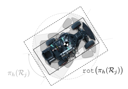
Note that in the interest of simplicity, we have abused notation and assumed that the argument to rot is any subset of $\mathbb{R}$ . In fact, it must always be a $1$ -dimensional box. In addition note that $\texttt{rot}\big{(}\pi_{h}(\mathcal{R}_{j})\big{)}$ is a zonotope because the 2-dimenional box $\SS$ is equivalent to a 2-dimensional zonotope and it is multiplied by a matrix via (3). By applying geometry, one can verify that by definition $\SS$ bounds the area that $\mathcal{O}^{\text{ego}}=\texttt{int}([-0.5L,-0.5W]^{\top},[0.5L,0.5W]^{\top})$ travels through while rotating within the range $[-h^{\text{rad}},h^{\text{rad}}]$ . As a result, $\texttt{rot}\big{(}\pi_{h}(\mathcal{R}_{j})\big{)}$ over-approximates the area over which $\mathcal{O}^{\text{ego}}$ sweeps according to $\pi_{h}(\mathcal{R}_{j})$ as shown in Fig. 4.

Because $\SS$ can be represented as a zonotope with 2 generators, one can denote $\texttt{rot}(\pi_{h}(\mathcal{R}_{j}))$ as $\text{\textless}c_{\texttt{rot}},\;G_{\texttt{rot}}\text{\textgreater}\subset\mathbb{R}^{2}$ where $G_{\texttt{rot}}\in\mathbb{R}^{2\times 2}$ . Notice $\texttt{rot}(\pi_{h}(\mathcal{R}_{j}))$ in (47) is a set in $\mathcal{W}$ rather than the higher dimensional space where $\mathcal{R}_{j}$ exists. We extend $\texttt{rot}(\pi_{h}(\mathcal{R}_{j}))$ to $\mathbb{R}^{9+n_{p}}$ as

\texttt{ROT}(\pi_{h}(\mathcal{R}_{j})):=\left<\begin{bmatrix}c_{\texttt{rot}}\\ 0_{(7+n_{p})\times 1}\end{bmatrix},~{}\begin{bmatrix}G_{\texttt{rot}}\\ 0_{(7+n_{p})\times 2}\end{bmatrix}\right>.

(48)

Using this definition, one can extend the FRS to account for the vehicle footprint as in the following lemma whose proof can be found in Appendix C:

Lemma 21.

Let $\{\mathcal{R}_{j}\}_{j\in\mathcal{J}}$ be the set of zonotopes computed by CORA under the hybrid vehicle dynamics model beginning from $\mathcal{Z}^{\text{aug}}_{0}$ . Let $z^{\text{aug}}$ be a solution to $HS$ with initial velocity $z^{\text{vel}}_{0}$ and control parameter $p$ and let $\xi:P(\mathbb{R}^{9+n_{p}})\times\mathcal{Z}^{\text{vel}}_{0}\times\mathcal{P}\rightarrow P(\mathcal{W})$ be defined as

\xi(\mathcal{R}_{j},z^{\text{vel}}_{0},p)=\pi_{xy}\Big{(}\texttt{slice}\big{(}\mathcal{R}_{j}\oplus\texttt{ROT}(\pi_{h}(\mathcal{R}_{j})),z^{\text{vel}}_{0},p\big{)}\Big{)}.

(49)

Then $\xi(\mathcal{R}_{j},z^{\text{vel}}_{0},p)$ is a zonotope and for all $j\in\mathcal{J}$ and $t\in T_{j}$ , the vehicle footprint oriented and centered according to $z^{\text{aug}}(t)$ is contained within $\xi(\mathcal{R}_{j},z^{\text{vel}}_{0},p)$ .

Again note that in the interest of simplicity we have abused notation and assumed that the first argument to $\xi$ is any subset of $\mathbb{R}^{9+n_{p}}$ . This argument is always a zonotope in $\mathbb{R}^{9+n_{p}}$ .

VII Online Planning

This section begins by taking nonzero initial position condition into account and formulating the optimization for online planning in REFINE to search for a safety guaranteed control policy in real time. It then explains how to represent each of the constraints of the online optimization problem in a differentiable fashion, and concludes by describing the performance of the online planning loop.

Before continuing we make an assumption regarding predictions of surrounding obstacles. Because prediction is not the primary emphasis of this work, we assume that the future position of any sensed obstacle within the sensor horizon during $[t_{0},t_{0}+t_{\text{plan}}+t_{\text{f}}]$ is conservatively known at time $t_{0}$ :

Assumption 22.

There exists a map $\vartheta:\mathcal{J}\times\mathcal{I}\rightarrow P(\mathcal{W})$ such that $\vartheta(j,i)$ is a zonotope and

\cup_{t\in T_{j}}\mathcal{O}_{i}(t)\cap\mathcal{B}\left((x(t_{0}),y(t_{0})),S\right)\subseteq\vartheta(j,i).

(50)

VII-A Nonzero Initial Position

Recall that the FRS computed in Section VI is computed offline while assuming that the initial position of the ego vehicle is zero (i.e., Assumption 15). The zonotope collection $\{\mathcal{R}_{j}\}_{j\in\mathcal{J}}$ can be understood as a local representation of the FRS in the local frame. This local frame is oriented at the ego vehicle’s location $[x_{0},y_{0}]^{\top}\in\mathbb{R}^{2}$ with its $x$ -axis aligned according to the ego vehicle’s heading $h_{0}\in\mathbb{R}$ , where $z^{\text{pos}}_{0}=[x_{0},y_{0},h_{0}]^{\top}$ gives the ego vehicle’s position $[x(t),y(t),h(t)]^{\top}$ at time $t=0$ in the world frame. Similarly, $\xi(\mathcal{R}_{j},z^{\text{vel}}_{0},p)$ is a local representation of the area that the ego vehicle may occupy during $T_{j}$ in the same local frame.

Because obstacles are defined in the world frame, to generate not-at-fault trajectories, one has to either transfer $\xi(\mathcal{R}_{j},z^{\text{vel}}_{0},p)$ from the local frame to the world frame, or transfer the obstacle position $\vartheta(j,i)$ from the world frame to the local frame using a 2D rigid body transformation. This work utilizes the second option and transforms $\vartheta(j,i)$ into the local frame as

\vartheta^{\text{loc}}(j,i,z^{\text{pos}}_{0})=\begin{bmatrix}\cos(h_{0})&\sin(h_{0})\\ -\sin(h_{0})&\cos(h_{0})\end{bmatrix}(\vartheta(j,i)-\begin{bmatrix}x_{0}\\ y_{0}\end{bmatrix}).

(51)

VII-B Online Optimization

Given the predicted initial condition of the vehicle at $t=0$ as $z_{0}=[(z^{\text{pos}}_{0})^{\top},(z^{\text{vel}}_{0})^{\top}]^{\top}\in\mathbb{R}^{3}\times\mathcal{Z}^{\text{vel}}_{0}$ , REFINE computes a not-at-fault trajectory by solving the following optimization problem at each planning iteration:

	$\displaystyle\min_{p\in\mathcal{P}}$	$\displaystyle\quad\texttt{cost}(z_{0},p)\hskip 113.81102pt(\texttt{Opt})$
	s.t.	$\displaystyle\quad\xi(\mathcal{R}_{j},z^{\text{vel}}_{0},p)\cap\vartheta^{\text{loc}}(j,i,z^{\text{pos}}_{0})=\emptyset,\hskip 14.22636pt\forall j\in\mathcal{J},\forall i\in\mathcal{I}$

where $\texttt{cost}:\mathbb{R}^{3}\times\mathcal{Z}^{\text{vel}}_{0}\times\mathcal{P}\to\mathbb{R}$ is a user-specified cost function and $\xi$ is defined as in Lemma 21. Note that the constraint in (Opt) is satisfied if for a particular trajectory parameter $p$ , there is no intersection between any obstacle and the reachable set of the ego vehicle with its footprint considered during any time interval while following $p$ .

VII-C Representing the Constraint and its Gradient in (Opt)

The following theorem, whose proof can be found in Appendix D, describes how to represent the set intersection constraint in (Opt) and how to compute its derivative with respect to $p\in\mathcal{P}$ :

Theorem 23.

There exists matrices $A$ and $B$ and a vector $b$ such that $\xi(\mathcal{R}_{j},z^{\text{vel}}_{0},p)\cap\vartheta^{\text{loc}}(j,i,z^{\text{pos}}_{0})=\emptyset$ if and only if $\max(BA\cdot p-b)>0$ . In addition, the subgradient of $\max(BA\cdot p-b)$ with respect to $p$ is $\max_{k\in\hat{K}}[BA]_{k:}$ , where $\hat{K}=\{k\mid[BA\cdot p-b]_{k}=\max(BA\cdot p-b)\}$ .

Formulas for the matrices $A$ and $B$ and vector $b$ in the previous theorem can be found in (88), (90), and (91), respectively.

VII-D Online Operation

Algorithm 1 summarizes the online operations of REFINE. In each planning iteration, the ego vehicle executes the feasible control parameter that is computed in the previous planning iteration (Line 3). Meanwhile, SenseObstacles senses and predicts obstacles as in Assumption 22 (Line 4) in local frame decided by $z^{\text{pos}}_{0}$ . (Opt) is then solved to compute a control parameter $p^{*}$ using $z_{0}$ and $\{\vartheta^{\text{loc}}(j,i,z^{\text{pos}}_{0})\}_{(j,i)\in\mathcal{J}\times\mathcal{I}}$ (Line 5). If (Opt) fails to find a feasible solution within $t_{\text{plan}}$ , the contingency braking maneuver whose safety is verified in the last planning iteration is executed, and REFINE is terminated (Line 6). In the case when (Opt) is able to find a feasible $p^{*}$ , StatePrediction predicts the state value at $t=t_{\text{m}}$ based on $z_{0}$ and $p^{*}$ as in Assumption 6 (Lines 7 and 8). If the predicted velocity value does not belong to $\mathcal{Z}^{\text{vel}}_{0}$ , then its corresponding FRS is not available and the planning has to stop while executing a braking maneuver (Line 9). Otherwise we reset time to 0 (Line 10) and start the next planning iteration. Note Lines 4 and 7 are assumed to execute instantaneously, but in practice the time spent for these steps can be subtracted from $t_{\text{plan}}$ to ensure real-time performance. By iteratively applying Definition 8, Lemmas 14 and 21, Assumption 22 and (51), the following theorem holds:

Theorem 24.

Suppose the ego vehicle can sense and predict surrounding obstacles as in Assumption 22, and starts with a not-at-fault control parameter $p_{0}\in\mathcal{P}$ . Then by performing planning and control as in Algorithm 1, the ego vehicle is not-at-fault for all time.

Algorithm 1 REFINE Online Planning

p_{0}\in\mathcal{P}

and

z_{0}=[(z^{\text{pos}}_{0})^{\top},(z^{\text{vel}}_{0})^{\top}]^{\top}\in\mathbb{R}^{3}\times\mathcal{Z}^{\text{vel}}_{0}

1: Initialize:

p^{*}=p_{0}

t=0

2: Loop: // Line 3 executes at the same time as Line 4-8

3: Execute

p^{*}

during

[0,t_{\text{m}})

\{\vartheta^{\text{loc}}(j,i,z^{\text{pos}}_{0})\}_{(j,i)\in\mathcal{J}\times\mathcal{I}}\leftarrow\texttt{SenseObstacles}()

5: Try

p^{*}\leftarrow\texttt{OnlineOpt}(z_{0},\{\vartheta^{\text{loc}}(j,i,z^{\text{pos}}_{0})\}_{(j,i)\in\mathcal{J}\times\mathcal{I}})

// within

t_{\text{plan}}

seconds

6: Catch execute

p^{*}

during

[t_{\text{m}},t_{\text{f}}]

, then break

(z^{\text{pos}}_{0},z^{\text{vel}}_{0})\leftarrow\texttt{StatePrediction}(z_{0},p^{*},t_{\text{m}})

z_{0}\leftarrow[(z^{\text{pos}}_{0})^{\top},(z^{\text{vel}}_{0})^{\top}]^{\top}

9: If (

z^{\text{vel}}_{0}\notin\mathcal{Z}^{\text{vel}}_{0}

), execute

p^{*}

during

[t_{\text{m}},t_{\text{f}}]

and break

10: Reset

t

to 0

11: End

VIII Extensions

This section describes how to extend various components of REFINE. This section begins by describing how to apply CORA to compute tight, conservative approximations of the FRS. Next, it illustrates how to verify the satisfaction of Assumption 3. The section concludes by describing how to apply REFINE to AWD and RWD vehicles.

VIII-A Subdivision of Initial Set and Families of Trajectories

In practice, CORA may generate overly conservative representations for the FRS if the initial condition set is large. To address this challenge, one can instead partition $\mathcal{Z}_{0}$ and $\mathcal{P}$ and compute a FRS beginning from each element in this partition. Note one could then still apply REFINE as in Algorithm 1. However in Line 5 must solve multiple optimizations of the form (Opt) in parallel. Each of these optimizations optimizes over a unique partition element that contains initial condition $z_{0}$ , then $p^{*}$ is set to be the feasible control parameter that achieves the minimum cost function value among these optimizations. Similarly note if one had multiple classes of desired trajectories (e.g. lane change, longitudinal speed changes, etc.) that were each parameterized in distinct ways, then one could extend REFINE just as in the instance of having a partition of the initial condition set. In this way one could apply REFINE to optimize over multiple families of desired trajectories to generate not-at-fault behavior. Note, that the planning horizon $t_{\text{f}}$ is constant within each element of the partition, but can vary between different elements in the partition.

VIII-B Satisfaction of Assumption 3

Throughout our analysis thus far, we assume that the slip ratios and slip angles stay within the linear regime as described in Assumption 3. This subsection describes how to ensure that Assumption 3 is satisfied by performing an offline verification on the computed reachable sets.

Recall that in an FWD vehicle model, $F_{\text{xr}}(t)=0$ for all $t$ as in Remark 2. By plugging (12) in (21), one can derive:

\begin{split}\lambda_{\text{f}}(t)=&\frac{l}{gl_{\text{r}}\bar{\mu}}\big{(}-K_{u}u(t)+K_{u}u^{\text{des}}(t,p)+\\ &+\dot{u}^{\text{des}}(t,p)-v(t)r(t)+\tau_{u}(t,p)\big{)}.\end{split}

(52)

Similarly by plugging (13) in (27) one can derive:

\begin{split}\alpha_{\text{f}}(t)=&-\frac{I_{\text{zz}}K_{r}}{l_{\text{f}}\bar{c}_{\alpha\text{f}}}\left(r(t)-r^{\text{des}}(t,p)\right)+\\ &-\frac{I_{\text{zz}}K_{h}}{l_{\text{f}}\bar{c}_{\alpha\text{f}}}\left(h(t)-h^{\text{des}}(t,p)\right)+\\ &+\frac{I_{\text{zz}}}{l_{\text{f}}\bar{c}_{\alpha\text{f}}}\dot{r}^{\text{des}}(t,p)+\frac{l_{\text{r}}}{l_{\text{f}}\bar{c}_{\alpha\text{f}}}F_{\text{yr}}(t)+\frac{I_{\text{zz}}}{l_{\text{f}}\bar{c}_{\alpha\text{f}}}\tau_{r}(t,p).\end{split}

(53)

If the slip ratio and slip angle computed in (52) and (53) satisfy Assumption 3, they achieve the expected tire forces as introduced in Section V-A.

By Definition 1 any $\mathcal{R}_{j}=\text{\textless}c_{\mathcal{R}_{j}},\;G_{\mathcal{R}_{j}}\text{\textgreater}$ that is computed by CORA under the hybrid vehicle dynamics model from a partition element in Section VIII-A, can be bounded by a multi-dimensional box $\texttt{int}(c_{\mathcal{R}_{j}}-|G_{\mathcal{R}_{j}}|\cdot\mathbf{1},c_{\mathcal{R}_{j}}+|G_{\mathcal{R}_{j}}|\cdot\mathbf{1})$ where $\mathbf{1}$ is a column vector of ones. This multi-dimensional box gives interval ranges of all elements in $z^{\text{aug}}$ during $T_{j}$ , which allows us to conservatively estimate $\{|\alpha_{\text{r}}(t)|\}_{t\in T_{j}}$ , $\{\mathcal{F}_{\text{yr}}(t)\}_{t\in T_{j}}$ and $\{|\lambda_{\text{f}}(t)|\}_{t\in T_{j}}$ via (9), (13) and (52) respectively using Interval Arithmetic [34]. The approximation of $\{\mathcal{F}_{\text{yr}}(t)\}_{t\in T_{j}}$ makes it possible to over-approximate $\{|\alpha_{\text{f}}(t)|\}_{t\in T_{j}}$ via (53).

Note in (52) and (53) integral terms are embedded in $\tau_{u}(t,p)$ and $\tau_{r}(t,p)$ as described in (22) and (28). Because it is nontrivial to perform Interval Arithmetic over integrals, we extend $z^{\text{aug}}$ to $z^{\text{aug}+}$ by appending three more auxiliary states $\varepsilon_{u}(t):=\int_{t_{0}}^{t}\|u(s)-u^{\text{des}}(s,p)\|^{2}ds$ , $\varepsilon_{r}(t):=\int_{t_{0}}^{t}\|r(s)-r^{\text{des}}(s,p)\|^{2}ds$ and $\varepsilon_{h}(t):=\int_{t_{0}}^{t}\|h(s)-h^{\text{des}}(s,p)\|^{2}ds$ . Notice

\begin{bmatrix}\dot{\varepsilon}_{u}(t)\\ \dot{\varepsilon}_{r}(t)\\ \dot{\varepsilon}_{h}(t)\end{bmatrix}=\begin{bmatrix}\|u(t)-u^{\text{des}}(t,p)\|^{2}\\ \|r(t)-r^{\text{des}}(t,p)\|^{2}\\ \|h(t)-h^{\text{des}}(t,p)\|^{2}\end{bmatrix},

(54)

then we can compute a higher-dimensional FRS of $z^{\text{aug}+}$ during $[0,t_{\text{f}}]$ through the same process as described in Section VI. This higher-dimensional FRS makes over-approximations of $\{\varepsilon_{u}(t)\}_{t\in\mathcal{T}_{j}}$ , $\{\varepsilon_{r}(t)\}_{t\in\mathcal{T}_{j}}$ and $\{\varepsilon_{h}(t)\}_{t\in\mathcal{T}_{j}}$ available for computation in (52) and (53).

If the supremum of $\{|\lambda_{\text{f}}(t)|\}_{t\in T_{j}}$ exceeds $\lambda^{\text{cri}}$ or any supremum of $\{|\alpha_{\text{f}}(t)|\}_{t\in T_{j}}$ and $\{|\alpha_{\text{r}}(t)|\}_{t\in T_{j}}$ exceeds $\alpha^{\text{cri}}$ , then the corresponding partition section of $\mathcal{Z}_{0}\times\mathcal{P}$ may result in a system trajectory that violates Assumption 3. Therefore to ensure not-at-fault, we only run optimization over partition elements whose FRS outer-approximations satisfy Assumption 3. Finally we emphasize that such verification of Assumption 3 over each partition element that is described in Section VIII-A can be done offline.

VIII-C Generalization to All-Wheel-Drive and Rear-Wheel-Drive

This subsection describes how REFINE can be extended to AWD and RWD vehicles. AWD vehicles share the same dynamics as (14) in Section III with one exception. In an AWD vehicle, only the lateral rear tire force is estimated and all the other three tire forces are controlled by using wheel speed and steering angle. In particular, computations related to the lateral tire forces as (27) and (53) are identical to the FWD case . However, both the front and rear tires contribute nonzero longitudinal forces, and they can be specified by solving the following system of linear equations:

$\displaystyle l_{\text{f}}F_{\text{xf}}(t)$	$\displaystyle=l_{\text{r}}F_{\text{xr}}(t)$
$\displaystyle F_{\text{xf}}(t)+F_{\text{xr}}(t)$	$\displaystyle=-mK_{u}u(t)+mK_{u}u^{\text{des}}(t,p)+$	(55)
	$\displaystyle+m\dot{u}^{\text{des}}(t,p)-mv(t)r(t)+m\tau_{u}(t,p)$

Longitudinal tire forces $F_{\text{xf}}(t)$ and $F_{\text{xr}}(t)$ computed from (55) can then be used to compute wheel speed $\omega_{\text{f}}(t)=\omega_{\text{r}}(t)$ as in (36). In this formulation, (52) also needs to be modified to

\begin{split}\lambda_{\text{f}}(t)=\lambda_{\text{r}}(t)=&\frac{1}{g\bar{\mu}}\big{(}-K_{u}u(t)+K_{u}u^{\text{des}}(t,p)+\\ &+\dot{u}^{\text{des}}(t,p)-v(t)r(t)+\tau_{u}(t,p)\big{)}\end{split}

(56)

to verify Assumption 3 along the longitudinal direction. Compared to FWD, in RWD the longitudinal front tire force is $0$ and the longitudinal rear tire force is controlled. Thus one can generalize to RWD by switching all related computations on $F_{\text{xf}}(t)$ and $F_{\text{xr}}(t)$ from the FWD case.

IX Experiments

This section describes the implementation and evaluation of REFINE in simulation using a FWD, full-size vehicle model and on hardware using an AWD, $\frac{1}{10}$ th size race car model. Readers can find a link to the software implementation¹¹1https://github.com/roahmlab/REFINE and videos²²2https://drive.google.com/drive/folders/1bXl07gTnaA3rJBl7J05SL0tsfIJEDfKy?usp=sharing, https://drive.google.com/drive/folders/1FvGHuqIRQpDS5xWRgB30h7exmGTjRyel?usp=sharing online.

IX-A Desired Trajectories

As detailed in Section V-A, the proposed controller relies on desired trajectories of vehicle longitudinal speed and yaw rate satisfying Definition 7. To test the performance of the proposed controller and planning framework, we selected $3$ families of desired trajectories that are observed during daily driving. Each desired trajectory is the concatenation of a driving maneuver and a contingency braking maneuver. The driving maneuver is either a speed change, direction change, or lane change (i.e. each option corresponds to one of the $3$ families of desired trajectories). Moreover, each desired trajectory is parameterized by $p=[p_{u},p_{y}]^{\top}\in\mathcal{P}\subset\mathbb{R}^{2}$ where $p_{u}$ denotes desired longitudinal speed, and $p_{y}$ decides desired lateral displacement.

Assuming that the ego vehicle has initial longitudinal speed $u_{0}\in\mathbb{R}$ at time $0$ , the desired trajectory for longitudinal speed is the same for each of the $3$ families of desired trajectories:

u^{\text{des}}(t,p)=\begin{cases}u_{0}+\frac{p_{u}-u_{0}}{t_{\text{m}}}t,\hskip 5.69046pt\text{ if }0<t<t_{\text{m}}\\ u^{\text{brake}}(t,p),\hskip 21.05519pt\text{ if }t\geq t_{\text{m}}\end{cases}

(57)

where

u^{\text{brake}}(t,p)=\begin{cases}p_{u}+(t-t_{\text{m}})a^{\text{dec}},\\ \hskip 14.22636pt\text{if }p_{u}>u^{\text{cri}}\text{ and }t_{\text{m}}\leq t<t_{\text{m}}+\frac{u^{\text{cri}}-p_{u}}{a^{\text{dec}}}\\ 0,\hskip 4.26773pt\text{if }p_{u}>u^{\text{cri}}\text{ and }t\geq t_{\text{m}}+\frac{u^{\text{cri}}-p_{u}}{a^{\text{dec}}}\\ 0,\hskip 4.26773pt\text{if }p_{u}\leq u^{\text{cri}}\text{ and }t\geq t_{\text{m}}\end{cases}

(58)

with some deceleration $a^{\text{dec}}<0$ . Note by Definition 7 $t_{\text{stop}}$ can be specified as

t_{\text{stop}}=\begin{cases}t_{\text{m}}+\frac{u^{\text{cri}}-p_{u}}{a^{\text{dec}}},~{}\text{ if }p_{u}>u^{\text{cri}}\\ t_{\text{m}},\hskip 44.10185pt\text{ if }p_{u}\leq u^{\text{cri}}.\end{cases}

(59)

The desired longitudinal speed approaches $p_{u}$ linearly from $u_{0}$ before braking begins at time $t_{\text{m}}$ , then decreases to $u^{\text{cri}}$ with deceleration $a^{\text{dec}}$ and immediately drops down to 0 at time $t_{\text{stop}}$ . Moreover, one can verify that the chosen $u^{\text{des}}(t,p)$ in (57) satisfies the assumptions on desired longitudinal speed in Lemma 14.

Assuming the ego vehicle has initial heading $h_{0}\in[-\pi,\pi]$ at time $0$ , the desired heading trajectory varies among the different trajectory families. Specifically, for the trajectory family associated with speed change:

h^{\text{des}}(t,p)=h_{0},~{}\forall t\geq 0.

(60)

Desired heading trajectory for the trajectory family associated with direction change:

h^{\text{des}}(t,p)=\begin{cases}h_{0}+\frac{p_{y}t}{2}-\frac{p_{y}t_{\text{m}}}{4\pi}\sin\left(\frac{2\pi t}{t_{\text{m}}}\right),\text{ if }0\leq t<t_{\text{m}}\\ h_{0}+\frac{p_{y}t_{\text{m}}}{2},\hskip 69.70915pt\text{ if }t\geq t_{\text{m}}\end{cases}

(61)

and for the trajectory family associated with lane change:

h^{\text{des}}(t,p)=\begin{cases}h_{0}+h^{\text{des}}_{1}p_{y}\cdot\mathrm{e}^{-h^{\text{des}}_{2}(t-0.5t_{\text{m}})^{2}},\\ \hskip 108.12054pt\text{ if }0\leq t<t_{\text{m}}\\ h_{0},\hskip 82.51282pt~{}~{}~{}\text{ if }t\geq t_{\text{m}}\end{cases}

(62)

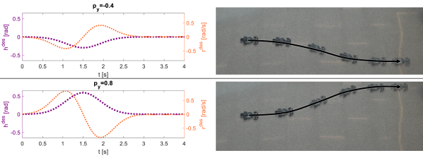
where $\mathrm{e}$ is Euler’s number, and $h^{\text{des}}_{1}$ and $h^{\text{des}}_{2}$ are user-specified auxiliary constants that adjust the desired heading amplitude. Illustrations of speed change and direction change maneuvers can be found in the software repository³³3https://github.com/roahmlab/REFINE/blob/main/Rover_Robot_Implementation/README.md#1-desired-trajectories. As shown in Figure 5, $h^{\text{des}}(t,p)$ remains constant for all $t\geq t_{\text{m}}$ among all families of desired trajectories. By Definition 7, desired trajectory of yaw rate is set as $r^{\text{des}}(t,p)=\frac{d}{dt}h^{\text{des}}(t,p)$ among all trajectory families.

In this work, $t_{\text{m}}$ for the speed change and direction change trajectory families are set equal to one another. $t_{\text{m}}$ for the lane change trajectory family is twice what it is for the direction change and speed change trajectory families. This is because a lane change can be treated as a concatenation of two direction changes. Because we do not know which desired trajectory ensures not-at-fault a priori, during each planning iteration, to guarantee real-time performance, $t_{\text{plan}}$ should be no greater than the smallest duration of a driving maneuver, i.e. speed change or direction change.

IX-B Simulation on a FWD Model

This subsection describes the evaluation of REFINE in simulation. In particular, this section describes the simulation environment, how we implement REFINE, the methods we compare it to, and the results of the evaluation.

IX-B1 Simulation Environment

We evaluate the performance on $1000$ randomly generated $3$ -lane highway scenarios in which the same full-size, FWD vehicle as the ego vehicle is expected to autonomously navigate through dynamic traffic for $1$ [km] from a fixed initial condition. All lanes of all highway scenario share the same lane width as $3.7$ [m]. Each highway scenario contains up to $24$ moving vehicles and up to $5$ static vehicles that start from random locations and are all treated as obstacles to the ego vehicle. Moreover, each moving obstacle maintains its randomly generated highway lane and initial speed up to $25$ [m/s] for all time. Because each highway scenario is randomly generated, there is no guarantee that the ego vehicle has a path to navigate itself from the start to the goal. Such cases allow us to verify if the tested methods can still keep the ego vehicle safe even in infeasible scenarios. Parameters of the ego vehicle can be found in the software implementation readme⁴⁴4https://github.com/roahmlab/REFINE/blob/main/Full_Size_Vehicle_Simulation/README.md#vehicle-and-control-parameters.

During each planning iteration, all evaluated methods use the same high level planner. This high level planner generates waypoints by first choosing the lane on which the nearest obstacle ahead has the largest distance from the ego vehicle. Subsequently it picks a waypoint that is ahead of the ego vehicle and stays along the center line of the chosen lane. The cost function in (Opt) or in any of the evaluated optimization-based motion planning algorithms is set to be the Euclidean distance between the waypoint generated by the high level planner and the predicted vehicle location based on initial state $z_{0}$ and decision variable $p$ . All simulations are implemented and evaluated in MATLAB R2022a on a laptop with an Intel i7-9750H processor and 16GB of RAM.

IX-B2 REFINE Simulation Implementation

REFINE invokes C++ for the online optimization using IPOPT [35]. Parameters of REFINE’s controller are chosen to satisfy the conditions in Lemma 14 and can be found in the software implementation readme⁵⁵5https://github.com/roahmlab/REFINE/blob/main/Full_Size_Vehicle_Simulation/README.md#vehicle-and-control-parameters. REFINE tracks families of desired trajectories as described in Section IX-A with $\mathcal{P}=\{(p_{u},p_{y})\in[5,30]\times[-0.8,0.8]\mid p_{u}=u_{0}\text{ if }p_{y}\neq 0\}$ , $a^{\text{dec}}=-5.0[\text{m}/\text{s}^{2}]$ , $h^{\text{des}}_{1}=\frac{6\sqrt{2\mathrm{e}}}{11}$ and $h^{\text{des}}_{2}=\frac{121}{144}$ . The duration $t_{\text{m}}$ of driving maneuvers for each trajectory family is 3[s] for speed change, 3[s] for direction change and 6[s] for lane change, therefore $t_{\text{plan}}$ is set to be 3[s]. As discussed in Section VIII-A, during offline computation, we evenly partition the first and second dimensions of $\mathcal{P}$ into intervals of lengths $0.5$ and $0.4$ , respectively. For each partition element, $t_{\text{f}}$ is assigned to be the maximum possible value of $t_{\text{brake}}$ as computed in (82) in which $t_{\text{fstop}}$ is by observation no greater than 0.1[s]. An outer-approximation of the FRS is computed for every partition element of $\mathcal{P}$ using CORA with $\Delta t$ as $0.015$ [s], $0.010$ [s], $0.005$ [s] and $0.001$ [s]. Note, that we choose these different values of $\Delta t$ to highlight how this choice affects the performance of REFINE.

IX-B3 Other Implemented Methods

We compare REFINE against several state of the art trajectory planning methods: a baseline zonotope reachable set method [36], a Sum-of-Squares-based RTD (SOS-RTD) method [13], and an NMPC method using GPOPS-II [37].

The first trajectory planning method that we implement is a baseline zonotope based reachability method that selects a finite number of possible trajectories rather than a continuum of possible trajectories as REFINE does. This baseline method is similar to the classic funnel library approach to motion planning [12] in that it chooses a finite number of possible trajectories to track. The baseline method computes zonotope reachable sets using CORA with $\Delta t=0.010$ [s] over a sparse discrete control parameter space $\mathcal{P}^{\text{sparse}}:=\{(p_{u},p_{y})\in\{5,5.1,5.2,\ldots,30\}\times\{0,0.4\}\mid p_{u}=u_{0}\text{ if }p_{y}\neq 0\}$ and a dense discrete control parameter space $\mathcal{P}^{\text{dense}}:=\{(p_{u},p_{y})\in\{5,5.1,5.2,\ldots,30\}\times\{0,0.04,0.08,\ldots,0.8\}\mid p_{u}=u_{0}\text{ if }p_{y}\neq 0\}$ . We use $\mathcal{P}^{\text{sparse}}$ and $\mathcal{P}^{\text{dense}}$ to illustrate the challenges associated with applying this baseline method in terms of computation time, memory consumption, and the ability to robustly travel through complex simulation environments. During each planning iteration, the baseline method searches through the discrete control parameter space until a feasible solution is found such that the corresponding zonotope reachable sets have no intersection with any obstacles over the planning horizon. The search procedure over this discrete control space is biased to select the same trajectory parameter that worked in the prior planning iteration or to search first from trajectory parameter that are close to one that worked in the previous planning iteration.

The SOS-RTD plans a controller that also tracks families of trajectories to achieve speed change, direction change and lane change maneuvers with braking maneuvers as described in Section IX-A. SOS-RTD offline approximates the FRS by solving a series of polynomial optimizations using Sum-of-Squares so that the FRS can be over-approximated as a union of superlevel sets of polynomials over successive time intervals of duration 0.1[s] [13]. Computed polynomial FRS are further expanded to account for footprints of other vehicles offline in order to avoid buffering each obstacle with discrete points online [16]. During online optimization, SOS-RTD plans every $3$ [s] and uses the same cost function as REFINE does, but checks collision against obstacles by enforcing that no obstacle has its center stay inside the FRS approximation during any time interval.

The NMPC method does not perform offline reachability analysis. Instead, it directly computes the control inputs that are applicable for $t_{\text{m}}$ seconds by solving an optimal control problem. This optimal control problem is solved using GPOPS-II in a receding horizon fashion. The NMPC method conservatively ensures collision-free trajectories by covering the footprints of the ego vehicle and all obstacles with two overlapping balls, and requiring that no ball of the ego vehicle intersects with any ball of any obstacle. Notice during each online planning iteration, the NMPC method does not need pre-defined desired trajectories for solving control inputs. Moreover, it does not require the planned control inputs to stop the vehicle by the end of planned horizon as the other three methods do.

Method	Safely Stop	Crash	Success	Average Travel Speed	Solving Time of Online Planning	Memory
Method	Safely Stop	Crash	Success	Average Travel Speed	(Average, Maximum)	Memory
Baseline (sparse, $\Delta t=0.010$ )	38%	0%	62%	22.3572[m/s]	(2.03[s], 4.15[s])	980 MB
Baseline (dense, $\Delta t=0.010$ )	30%	0%	70%	23.6327[m/s]	(12.42[s], 27.74[s])	9.1 GB
SOS-RTD	36%	0%	64%	24.8049[m/s]	(0.05[s], 1.58[s])	2.4 GB
NMPC	3%	29%	68%	27.3963[m/s]	(40.89[s], 534.82[s])	N/A
REFINE ( $\Delta t=0.015$ )	27%	0%	73%	23.2452[m/s]	(0.34[s], 0.95[s])	488 MB
REFINE ( $\Delta t=0.010$ )	17%	0%	83%	24.8311[m/s]	(0.52[s], 1.57[s])	703 MB
REFINE ( $\Delta t=0.005$ )	16%	0%	84%	24.8761[m/s]	(1.28[s], 4.35[s])	997 MB
REFINE ( $\Delta t=0.001$ )	16%	0%	84%	24.8953[m/s]	(6.48[s], 10.78[s])	6.4 GB

TABLE I: Summary of performance of various tested techniques on the same

1000

simulation environments.

IX-B4 Evaluation Criteria

We evaluate each implemented trajectory planning method in several ways as summarized in Table I First, we report the percentage of times that each planning method either came safely to a stop (in a not-at-fault manner), crashed, or successfully navigated through the scenario. Note a scenario is terminated when one of those three conditions is satisfied. Second, we report the average travel speed during all scenarios. Third, we report the average and maximum planning time over all scenarios. Finally, we report on the size of the pre-computed reachable set.

IX-B5 Results

REFINE achieves the highest success rate among all evaluated methods and has no crashes. The success rate of REFINE converges to 84% as the value of $\Delta t$ decreases because the FRS approximation becomes tighter with denser time discretization. However as the time discretization becomes finer, memory consumption grows larger because more zonotopes are used to over-approximate FRS. Furthermore, due to the increasing number of zonotope reachable sets, the solving time also increases and begins to exceed the allotted planning time. According to our simulation, we see that $\Delta t=0.010$ [s] results in high enough successful rate while maintaining a planning time no greater than $3$ [s].

The baseline method with $\mathcal{P}^{\text{sparse}}$ shares almost the same memory consumption as REFINE with $\Delta t=0.005$ [s], but results in a much lower successful rate and smaller average travel speed. When the baseline method runs over $\mathcal{P}^{\text{dense}}$ , its success rate is increased, but still smaller than that of REFINE. More troublingly, its memory consumption increases to $9.1$ GB. Neither evaluated baseline is able to finish online planning within $3$ [s]. Compared to REFINE, SOS-RTD completes online planning faster and can also guarantee vehicle safety with a similar average travel speed. However SOS-RTD needs a memory of $2.4$ GB to store its polynomial reachable sets, and its success rate is only $64$ % because the polynomial reachable sets are more conservative than zonotope reachable sets.

When the NMPC method is utilized for motion planning, the ego vehicle achieves a similar success rate as SOS-RTD, but crashes occur $29$ % of the time. Note the NMPC method achieves a higher average travel speed of the ego vehicle when compared to the other three methods. More aggressive operation can allow the ego vehicle drive closer to obstacles, but can make subsequent obstacle avoidance difficult. The NMPC method uses $40.8906$ [s] on average to compute a solution, which makes real-time path planning untenable.

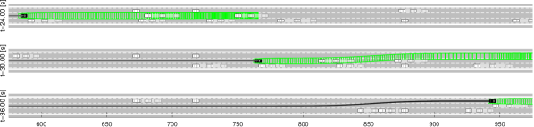
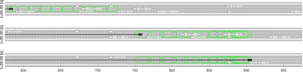
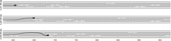
Figure 6 illustrates the performance of the three methods in the same scene at three different time instances. In Figure 6(a), because REFINE gives a tight approximation of the ego vehicle’s FRS using zonotopes, the ego vehicle is able to first bypass static vehicles in the top lane from $t=24$ [s] to $t=30$ [s], then switch to the top lane and bypass vehicles in the middle lane from $t=30$ [s] to $t=36$ [s]. In Figure 6(b) SOS-RTD is used for planning. In this case the ego vehicle bypasses the static vehicles in the top lane from $t=24$ [s] to $t=30$ [s]. However because online planing becomes infeasible due to the conservatism of polynomial reachable sets, the ego vehicle executes the braking maneuver to stop itself $t=30$ [s] to $t=36$ [s]. In Figure 6(c) because NMPC is used for planning, the ego vehicle drives at a faster speed and arrives at $600$ [m] before the other evaluated methods. Because the NMPC method only enforces collision avoidance constraints at discrete time instances, the ego vehicle ends up with a crash at $t=24$ [s] though NMPC claims to find a feasible solution for the planning iteration at $t=21$ [s].

IX-C Real World Experiments

REFINE was also implemented in C++17 and tested in the real world using a $\frac{1}{10}$ th All-Wheel-Drive car-like robot, Rover, based on a Traxxax RC platform. The Rover is equipped with a front-mounted Hokuyo UST-10LX 2D lidar that has a sensing range of 10[m] and a field of view of 270°. The Rover is equipped with a VectorNav VN-100 IMU unit which publishes data at 800Hz. Sensor drivers, state estimator, obstacle detection, and the proposed controller are run on an NVIDIA TX-1 on-board computer. A standby laptop with Intel i7-9750H processor and 32GB of RAM is used for localization, mapping, and solving (Opt) in over multiple partitions of $\mathcal{P}$ . The rover and the standby laptop communicate over wifi using ROS [38].

The desired trajectories on the Rover are parameterized with $\mathcal{P}=\{(p_{u},p_{y})\in[0.05,2.05]\times[-1.396,1.396]\mid p_{u}=u_{0}\text{ if }p_{y}\neq 0\}$ , $a^{\text{dec}}=-1.5$ [m/sec²], $h^{\text{des}}_{1}=\frac{20}{27}$ and $h^{\text{des}}_{2}=\frac{27}{10}$ as described in Section IX-A. The duration $t_{\text{m}}$ of driving maneuvers for each trajectory family is set to $1.5$ [s] for speed change, $1.5$ [s] for direction change, and $3$ [s] for lane change, thus planning time for real world experiments is set as $t_{\text{plan}}=1.5$ [s]. The parameter space $\mathcal{P}$ is evenly partitioned along its first and second dimensions into small intervals of lengths 0.25 and 0.349, respectively. For each partition element, $t_{\text{f}}$ is set equal to the maximum possible value of $t_{\text{brake}}$ as computed in (82) in which $t_{\text{fstop}}$ is by observation no greater than 0.1[s]. The FRS of the Rover for every partition element of $\mathcal{P}$ is overapproximated using CORA with $\Delta t=0.01$ [s]. During online planning, a waypoint is selected in real time using Dijkstra’s algorithm [39], and the cost function of (Opt) is set in the same way as we do in simulation as described in Section IX-B. The robot model, environment sensing, and state estimation play key roles in real world experiments. In the rest of this subsection, we describe how to bound the modeling error in (14) and summarize the real world experiments. Details regarding Rover model parameters, the controller parameters, how the Rover performs localization, mapping, and obstacle detection and how we perform system identification of the tire models can be found in our software implementation readme⁶⁶6https://github.com/roahmlab/REFINE/blob/main/Rover_Robot_Implementation/README.md.

IX-C1 State Estimation and System Identification on Model Error in Vehicle Dynamics

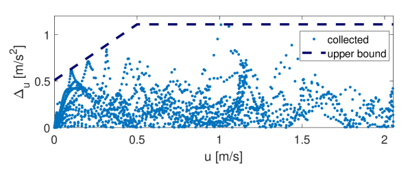
The modeling error in the dynamics (14) arise from ignoring aerodynamic drag force and the inaccuracies of state estimation and the tire models. We use the data collected to fit the tire models to identify the modeling errors $\Delta_{u}$ , $\Delta_{v}$ , and $\Delta_{r}$ .

We compute the model errors as the difference between the actual accelerations collected by the IMU and the estimation of applied accelerations computed via (4) in which tire forces are calculated via (12) and (13). The estimation of applied accelerations is computed using the estimated system states via an Unscented Kalman Filter (UKF) [40], which treats SLAM results, IMU readings, and encoding information of wheel and steering motors as observed outputs of the Rover model. The robot dynamics that UKF uses to estimate the states is the error-free, high-speed dynamics (4) with linear tire models. Note the UKF state estimator is still applicable in the low-speed case except the estimation of $v$ and $r$ are ignored. To ensure $\Delta_{u}$ , $\Delta_{v}$ and $\Delta_{r}$ are square integrable, we set $\Delta_{u}(t)=\Delta_{v}(t)=\Delta_{r}(t)=0$ for all $t\geq t_{\text{brake}}$ where $t_{\text{brake}}$ is computed in Lemma 14. As shown in Figure 7 bounding parameters $M_{u}$ , $M_{v}$ , and $M_{r}$ are selected to be the maximum value of $|\Delta_{u}(t)|$ , $|\Delta_{v}(t)|$ , and $|\Delta_{r}(t)|$ respectively over all time, and $b_{u}^{\text{pro}}$ and $b_{u}^{\text{off}}$ are generated by bounding $|\Delta_{u}(t)|$ from above when $u(t)\leq u^{\text{cri}}$ .

IX-C2 Demonstration

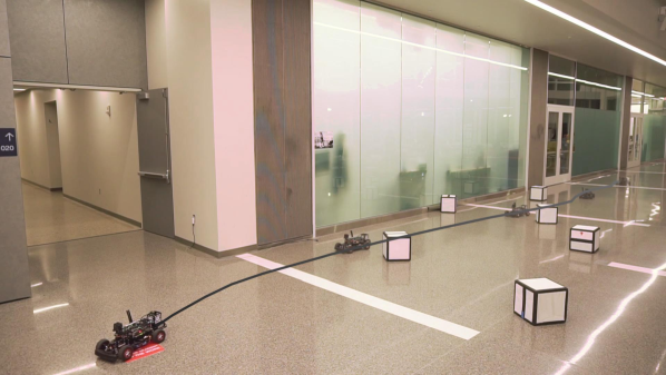
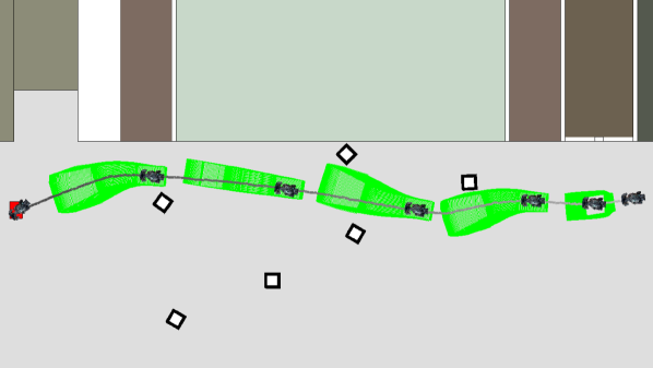
The Rover was tested indoors under the proposed controller and planning framework in 6 small trials and 1 loop trial⁷⁷7https://drive.google.com/drive/folders/1FvGHuqIRQpDS5xWRgB30h7exmGTjRyel?usp=sharing. In every small trail, up to $11$ identical $0.3\times 0.3\times 0.3$ [m]³ cardboard cubes were placed in the scene before the Rover began to navigate itself. The Rover was not given prior knowledge of the obstacles for each trial. Figure 8 illustrates the scene in the 6th small trial and illustrates REFINE’s performance. The zonotope reachable sets over-approximate the trajectory of the Rover and never intersect with obstacles.

In the loop trial, the Rover was required to perform 3 loops, and each loop is about 100[m] in length. In the first loop of the loop trial, no cardboard cube was placed in the loop, while in the last two loops the cardboard cubes were randomly thrown at least 5[m] ahead of the running Rover to test its maneuverability and safety. During the loop trial, the Rover occasionally stoped because a randomly thrown cardboard cube might be close to a waypoint or the end of an executing maneuver. In such cases, because the Rover was able to eventually locate obstacles more accurately when it was stopped, the Rover began a new planning iteration immediately after stopping and passed the cube when a feasible plan with safety guaranteed was found.

For all 7 real-world testing trials, the Rover either safely finishes the given task, or it stops itself before running into an obstacle if no clear path is found. The Rover is able to finish all computation of a planning iteration within 0.4021[s] on average and 0.6545[s] in maximum, which are both smaller than $t_{\text{plan}}=1.5$ [s], thus real-time performance is achieved.

X Conclusion

This work presents a controller-oriented trajectory design framework using zonotope reachable sets. A robust controller is designed to partially linearize the full-order vehicle dynamics with modeling error by performing feedback linearization on a subset of vehicle states. Zonotope-based reachability analysis is performed on the closed-loop vehicle dynamics for FRS computation, and achieves less conservative FRS approximation than that of the traditional reachability-based approaches. Tests on a full-size vehicle model in simulation and a 1/10th race car robot in real hardware experiments show that the proposed method is able to safely navigate the vehicle through random environments in real time and outperforms all evaluated state of the art methods.

References

[1] Steven M LaValle and James J Kuffner Jr “Randomized kinodynamic planning” In The international journal of robotics research 20.5 SAGE Publications, 2001, pp. 378–400
[2] Lucas Janson, Edward Schmerling, Ashley Clark and Marco Pavone “Fast marching tree: A fast marching sampling-based method for optimal motion planning in many dimensions” In The International journal of robotics research 34.7 SAGE Publications Sage UK: London, England, 2015, pp. 883–921
[3] Mohamed Elbanhawi and Milan Simic “Sampling-based robot motion planning: A review” In Ieee access 2 IEEE, 2014, pp. 56–77
[4] Steven M LaValle “Planning algorithms” Cambridge university press, 2006
[5] Yoshiaki Kuwata et al. “Real-time motion planning with applications to autonomous urban driving” In IEEE Transactions on control systems technology 17.5 IEEE, 2009, pp. 1105–1118
[6] Thomas M Howard and Alonzo Kelly “Optimal rough terrain trajectory generation for wheeled mobile robots” In The International Journal of Robotics Research 26.2 Sage Publications Sage CA: Thousand Oaks, CA, 2007, pp. 141–166
[7] Paolo Falcone et al. “Low complexity mpc schemes for integrated vehicle dynamics control problems” In 9th international symposium on advanced vehicle control (AVEC), 2008
[8] Chris Urmson et al. “Autonomous driving in urban environments: Boss and the urban challenge” In Journal of Field Robotics 25.8 Wiley Online Library, 2008, pp. 425–466
[9] John Wurts, Jeffrey L Stein and Tulga Ersal “Collision imminent steering using nonlinear model predictive control” In 2018 Annual American Control Conference (ACC), 2018, pp. 4772–4777 IEEE
[10] Matthias Althoff and John M Dolan “Online verification of automated road vehicles using reachability analysis” In IEEE Transactions on Robotics 30.4 IEEE, 2014, pp. 903–918
[11] Christian Pek, Stefanie Manzinger, Markus Koschi and Matthias Althoff “Using online verification to prevent autonomous vehicles from causing accidents” In Nature Machine Intelligence 2.9 Nature Publishing Group, 2020, pp. 518–528
[12] Anirudha Majumdar and Russ Tedrake “Funnel libraries for real-time robust feedback motion planning” In The International Journal of Robotics Research 36.8 SAGE Publications Sage UK: London, England, 2017, pp. 947–982
[13] Shreyas Kousik et al. “Bridging the gap between safety and real-time performance in receding-horizon trajectory design for mobile robots” In The International Journal of Robotics Research 39.12 SAGE Publications Sage UK: London, England, 2020, pp. 1419–1469
[14] Shreyas Kousik, Sean Vaskov, Matthew Johnson-Roberson and Ram Vasudevan “Safe trajectory synthesis for autonomous driving in unforeseen environments” In ASME 2017 Dynamic Systems and Control Conference, 2017 American Society of Mechanical Engineers Digital Collection
[15] Sean Vaskov et al. “Not-at-fault driving in traffic: A reachability-based approach” In 2019 IEEE Intelligent Transportation Systems Conference (ITSC), 2019, pp. 2785–2790 IEEE
[16] Sean Vaskov et al. “Towards provably not-at-fault control of autonomous robots in arbitrary dynamic environments” In arXiv preprint arXiv:1902.02851, 2019
[17] Somil Bansal, Mo Chen, Sylvia Herbert and Claire J Tomlin “Hamilton-jacobi reachability: A brief overview and recent advances” In 2017 IEEE 56th Annual Conference on Decision and Control (CDC), 2017, pp. 2242–2253 IEEE
[18] Sylvia L Herbert et al. “FaSTrack: A modular framework for fast and guaranteed safe motion planning” In 2017 IEEE 56th Annual Conference on Decision and Control (CDC), 2017, pp. 1517–1522 IEEE
[19] Reza N Jazar “Vehicle dynamics: theory and application” Springer, 2008 URL: https://link.springer.com/chapter/10.1007/978-0-387-74244-1_2
[20] A Galip Ulsoy, Huei Peng and Melih Çakmakci “Automotive control systems” Cambridge University Press, 2012
[21] Thomas D Gillespie “Fundamentals of vehicle dynamics”, 1992
[22] James Balkwill “Performance vehicle dynamics: engineering and applications” Butterworth-Heinemann, 2017
[23] S Dieter, M Hiller and R Baradini “Vehicle Dynamics: Modeling and Simulation” Springer-Verlag Berlin Heidelberg, Berlin, Germany, 2018
[24] Tae-Yun Kim, Samuel Jung and Wan-Suk Yoo “Advanced slip ratio for ensuring numerical stability of low-speed driving simulation: Part II—lateral slip ratio” In Proceedings of the Institution of Mechanical Engineers, Part D: Journal of automobile engineering 233.11 SAGE Publications Sage UK: London, England, 2019, pp. 2903–2911
[25] Reinhold Remmert “Theory of complex functions” Springer Science & Business Media, 1991
[26] Shai Shalev-Shwartz, Shaked Shammah and Amnon Shashua “On a formal model of safe and scalable self-driving cars” In arXiv preprint arXiv:1708.06374, 2017
[27] Ming-Yuan Yu, Ram Vasudevan and Matthew Johnson-Roberson “Occlusion-aware risk assessment for autonomous driving in urban environments” In IEEE Robotics and Automation Letters 4.2 IEEE, 2019, pp. 2235–2241
[28] Ming-Yuan Yu, Ram Vasudevan and Matthew Johnson-Roberson “Risk assessment and planning with bidirectional reachability for autonomous driving” In 2020 IEEE International Conference on Robotics and Automation (ICRA), 2020, pp. 5363–5369 IEEE
[29] Andrea Giusti and Matthias Althoff “Ultimate robust performance control of rigid robot manipulators using interval arithmetic” In 2016 American Control Conference (ACC), 2016, pp. 2995–3001 IEEE
[30] Jan Lunze and Françoise Lamnabhi-Lagarrigue “Handbook of hybrid systems control: theory, tools, applications” Cambridge University Press, 2009
[31] Matthias Althoff “An introduction to CORA 2015” In Proc. of the Workshop on Applied Verification for Continuous and Hybrid Systems, 2015
[32] Matthias Althoff “Reachability analysis and its application to the safety assessment of autonomous cars”, 2010
[33] Patrick Holmes et al. “Reachable sets for safe, real-time manipulator trajectory design (version 1)” https://arxiv.org/abs/2002.01591v1 In arXiv preprint arXiv:2002.01591, 2020
[34] Timothy Hickey, Qun Ju and Maarten H Van Emden “Interval arithmetic: From principles to implementation” In Journal of the ACM (JACM) 48.5 ACM New York, NY, USA, 2001, pp. 1038–1068
[35] Andreas Wächter and Lorenz T Biegler “On the implementation of an interior-point filter line-search algorithm for large-scale nonlinear programming” In Mathematical programming 106.1 Springer, 2006, pp. 25–57
[36] Stefanie Manzinger, Christian Pek and Matthias Althoff “Using reachable sets for trajectory planning of automated vehicles” In IEEE Transactions on Intelligent Vehicles 6.2 IEEE, 2020, pp. 232–248
[37] Michael A Patterson and Anil V Rao “GPOPS-II: A MATLAB software for solving multiple-phase optimal control problems using hp-adaptive Gaussian quadrature collocation methods and sparse nonlinear programming” In ACM Transactions on Mathematical Software (TOMS) 41.1 ACM New York, NY, USA, 2014, pp. 1–37
[38] Stanford Artificial Intelligence Laboratory et al. “Robotic Operating System”, 2018 URL: https://www.ros.org
[39] Edsger W Dijkstra “A note on two problems in connexion with graphs” In Numerische mathematik 1.1, 1959, pp. 269–271
[40] E.A. Wan and R. Van Der Merwe “The unscented Kalman filter for nonlinear estimation” In Proceedings of the IEEE 2000 Adaptive Systems for Signal Processing, Communications, and Control Symposium (Cat. No.00EX373), 2000, pp. 153–158 DOI: 10.1109/ASSPCC.2000.882463
[41] Leonidas J Guibas, An Thanh Nguyen and Li Zhang “Zonotopes as bounding volumes.” In SODA 3, 2003, pp. 803–812
[42] Elijah Polak “Optimization: algorithms and consistent approximations” Springer Science & Business Media, 2012

Appendix A Proof of Lemma 14

Proof.

This proof defines a Lyapunov function candidate and uses it to analyze the tracking error of the ego vehicle’s longitudinal speed before time $t_{\text{stop}}$ . Then it describes how $u$ evolves after time $t_{\text{stop}}$ in different scenarios depending on the value of $u(t_{\text{stop}})$ . Finally it describes how to set the time $t_{\text{brake}}$ to guarantee $u(t)=0$ for all $t\geq t_{\text{brake}}$ . For convenience, let $u^{\text{small}}:=\frac{M_{u}}{\kappa_{1,u}M_{u}+\phi_{1,u}}$ , then by assumption of the theorem $u^{\text{small}}\in(0.15,u^{\text{cri}}]$ . This proof suppresses the dependence on $p$ in $u^{\text{des}}(t,p)$ , $\tau_{u}(t,p)$ , $\kappa_{u}(t,p)$ , $\phi_{u}(t,p)$ and $e_{u}(t,p)$ .

Note by (25) and rearranging (26),

\dot{e}_{u}(t)=-K_{u}e_{u}(t)+\tau_{u}(t)+\Delta_{u}(t).

(63)

Recall $u^{\text{des}}$ is piecewise continuously differentiable by Definition 7, so are $e_{u}$ and $\tau_{u}$ . Without loss of generality we denote $\{t_{1},t_{2},\ldots,t_{k_{\text{max}}}\}$ a finite subdivision of $[0,t_{\text{stop}})$ with $t_{1}=0$ and $t_{k_{\text{max}}}=t_{\text{stop}}$ such that $u^{\text{des}}$ is continuously differentiable over time interval $[t_{k},t_{k+1})$ for all $k\in\{1,2,\ldots,k_{\text{max}}-1\}$ . Define $V(t):=\frac{1}{2}e_{u}^{2}(t)$ as a Lyapunov function candidate for $e_{u}(t)$ , then for arbitrary $k\in\{1,2,\ldots,k_{\text{max}}-1\}$ and $t\in[t_{k},t_{k+1})$ , one can check that $V(t)$ is always non-negative and $V(t)=0$ only if $e_{u}(t)=0$ . Then

$\displaystyle\dot{V}(t)$	$\displaystyle=e_{u}(t)\dot{e}_{u}(t)$	(64)
	$\displaystyle=-K_{u}e_{u}^{2}(t)+e_{u}(t)\tau_{u}(t)+e_{u}(t)\Delta_{u}(t)$	(65)
	$\displaystyle=-K_{u}e_{u}^{2}(t)-(\kappa_{u}(t)M_{u}+\phi_{u}(t))e_{u}^{2}(t)+$	(66)
	$\displaystyle\hskip 28.45274pt+e_{u}(t)\Delta_{u}(t)$	(67)

in which the second equality comes from (63) and the third equality comes from (22). Because the integral terms in (23) and (24) are both non-negative, $\kappa_{u}(t)\geq\kappa_{1,u}$ and $\phi_{u}(t)\geq\phi_{1,u}$ hold. Then

\begin{split}\dot{V}(t)\leq-K_{u}e_{u}^{2}(t)-(\kappa_{1,u}M_{u}+\phi_{1,u})|e_{u}(t)|^{2}+\\ +|e_{u}(t)||\Delta_{u}(t)|.\end{split}

(68)

By factoring out $|e_{u}(t)|$ in the last two terms in (68):

\dot{V}(t)\leq-K_{u}e_{u}^{2}(t)<0

(69)

holds when $|e_{u}(t)|>0$ and $|e_{u}(t)|\geq\frac{|\Delta_{u}(t)|}{\kappa_{1,u}M_{u}+\phi_{1,u}}$ . Note $|e_{u}(t)|\geq u^{\text{small}}$ conservatively implies $|e_{u}(t)|\geq\frac{|\Delta_{u}(t)|}{\kappa_{1,u}M_{u}+\phi_{1,u}}$ given $|\Delta_{u}(t)|\leq M_{u}$ for all time by Assumption 4. Then when $|e_{u}(t)|\geq u^{\text{small}}>0$ we have (69) hold, or equivalently $V(t)$ decreases. Therefore if $|e_{u}(t_{k})|\geq u^{\text{small}}$ , $|e_{u}(t)|$ monotonically decreases during time interval $[t_{k},t_{k+1})$ as long as $|e_{u}(t)|$ does not reach at the boundary of closed ball $\mathcal{B}(0,u^{\text{small}})$ . Moreover, if $|e_{u}(t^{\prime})|$ hits the boundary of $\mathcal{B}(0,u^{\text{small}})$ at some time $t^{\prime}\in[t_{k},t_{k+1})$ , $e_{u}(t)$ is prohibited from leaving the ball for all $t\in[t^{\prime},t_{k+1})$ because $\dot{V}(t)$ is strictly negative when $|e_{u}(t)|=u^{\text{small}}$ . Similarly $|e_{u}(t_{k})|\leq u^{\text{small}}$ implies $|e_{u}(t)|\leq u^{\text{small}}$ for all $t\in[t_{k},t_{k+1})$ .

We now analyze the behavior of $e_{u}(t)$ for all $t\in[0,t_{\text{stop}})$ . By assumption $u^{\text{des}}(0)=u(0)$ , then $|e_{u}(0)|=0<u^{\text{small}}$ and thus $|e_{u}(t)|\leq u^{\text{small}}$ for all $t\in[t_{1},t_{2})$ . Because both $u(t)$ and $u^{\text{des}}(t)$ are continuous during $[0,t_{\text{stop}})$ , so is $e_{u}(t_{2})$ . Thus $|e_{u}(t_{2})|\leq u^{\text{small}}$ . By iteratively applying the same reasoning, one can show that $|e_{u}(t)|\leq u^{\text{small}}$ for all $t\in[t_{k},t_{k+1})$ and for all $k\in\{1,2,\ldots,k_{\text{max}}-1\}$ , therefore $|e_{u}(t)|\leq u^{\text{small}}$ for all $t\in[0,t_{\text{stop}})$ . Furthermore, because $u^{\text{des}}(t)$ converges to $u^{\text{cri}}$ as $t$ converges to $t_{\text{stop}}$ from below, $u(t_{\text{stop}})\in[u^{\text{cri}}-u^{\text{small}},u^{\text{cri}}+u^{\text{small}}]$ . Note $u(t_{\text{stop}})\geq 0$ because $u^{\text{small}}\leq u^{\text{cri}}$ .

Next we analyze how longitudinal speed of the ego vehicle evolves after time $t_{\text{stop}}$ . Using $V(t)=\frac{1}{2}e_{u}^{2}(t)$ , we point out that (68) remains valid for all $t\geq t_{\text{stop}}$ , and (69) also holds when $|e_{u}(t)|\geq u^{\text{small}}$ with $t\geq t_{\text{stop}}$ . Recall $u(t)=e_{u}(t)$ for all $t\geq t_{\text{stop}}$ given $u^{\text{des}}(t)=0$ for all $t\geq t_{\text{stop}}$ , then for simplicity, the remainder of this proof replaces every $e_{u}(t)$ by $u(t)$ in (68), (69) and $V(t)$ . Because $u(0)>0$ and $u$ is continuous with respect to time, the longitudinal speed of the ego vehicle cannot decrease from a positive value to a negative value without passing 0. However when $u(t)=0$ , by Assumption 5 $\Delta_{u}(t)=0$ , thus $\dot{u}(t)=0$ by (26) given $u^{\text{des}}(t)=0$ for all $t\geq t_{\text{stop}}$ . In other words, once $u$ arrives at 0, it remains at 0 forever. For the ease of expression, from now on we assume $t\geq t_{\text{stop}}$ and $u(t)\geq 0$ for all $t\geq t_{\text{stop}}$ . Recall $u(t_{\text{stop}})\in[u^{\text{cri}}-u^{\text{small}},u^{\text{cri}}+u^{\text{small}}]$ and $u^{\text{cri}}-u^{\text{small}}\in[0,u^{\text{cri}}-0.15)$ . We now discuss how $u$ evolves after time $t_{\text{stop}}$ by considering three scenarios, and giving an upper bound of the time at when $u$ reaches 0 for each scenario.

Case 1 - When $u(t_{\text{stop}})\leq 0.15$ : Because the longitudinal speed stays at 0 once it becomes 0, by Assumption 13 the ego vehicle reaches to a full stop no later than $t_{\text{fstop}}+t_{\text{stop}}$ .

Case 2 - When $0.15<u(t_{\text{stop}})\leq u^{\text{small}}$ : By Assumption 5, upper bound of $\dot{V}(t)$ can be further relaxed from (68) to

\begin{split}\dot{V}(t)\leq-K_{u}u^{2}(t)-(\kappa_{1,u}M_{u}+\phi_{1,u}+\\ -b_{u}^{\text{pro}})u^{2}(t)+b_{u}^{\text{off}}u(t).\end{split}

(70)

Moreover, by completing the square among the last two terms in (70), one can derive

\dot{V}(t)\leq-K_{u}u^{2}(t)+\frac{(b_{u}^{\text{off}})^{2}}{4(\kappa_{1,u}M_{u}+\phi_{1,u}-b_{u}^{\text{pro}})}.

(71)

Notice $\frac{(b_{u}^{\text{off}})^{2}}{4(\kappa_{1,u}M_{u}+\phi_{1,u}-b_{u}^{\text{pro}})}<0.15^{2}K_{u}$ by assumption, thus

\dot{V}(t)<-K_{u}(u^{2}(t)-0.15^{2}).

(72)

This means as long as $u(t)\in[0.15,u^{\text{cri}}]$ with $t\geq t_{\text{stop}}$ , we obtain $\dot{V}(t)<0$ , or equivalently $V(t)=\frac{1}{2}u^{2}(t)$ decreases monotonically. Recall $u(t_{\text{stop}})\leq u^{\text{small}}\leq u^{\text{cri}}$ , then the longitudinal speed decreases monotonically from $u(t_{\text{stop}})$ to 0.15 as time increases from $t_{\text{stop}}$ . Suppose $u$ becomes 0.15 at time $t_{\text{brake}}^{\prime}\geq t_{\text{stop}}$ , then $u(t)\leq 0.15$ for all $t\geq t_{\text{brake}}^{\prime}$ because of the fact that $\dot{V}(t)$ is strictly negative when $u(t)=0.15$ .

Define $q_{u}:=\frac{(b_{u}^{\text{off}})^{2}}{4(\kappa_{1,u}M_{u}+\phi_{1,u}-b_{u}^{\text{pro}})}$ , then when $u(t)\in[0.15,u(t_{\text{stop}})]$ , (71) can be relaxed to

\dot{V}(t)\leq-K_{u}\cdot 0.15^{2}+q_{u}.

(73)

Integrate both sides of (73) from time $t_{\text{stop}}$ to $t_{\text{brake}}^{\prime}$ results in

t_{\text{brake}}^{\prime}\leq\frac{u(t_{\text{stop}})^{2}-0.15^{2}}{2\cdot 0.15^{2}K_{u}-2q_{u}}+t_{\text{stop}}.

(74)

Because $u(t_{\text{stop}})\leq u^{\text{small}}$ ,

t_{\text{brake}}^{\prime}\leq\frac{(u^{\text{small}})^{2}-0.15^{2}}{2\cdot 0.15^{2}K_{u}-2q_{u}}+t_{\text{stop}}.

(75)

Then $u$ becomes 0 no later than time $t_{\text{fstop}}+\sup(t_{\text{brake}}^{\prime})$ based on Assumption 13, where $\sup(t_{\text{brake}}^{\prime})$ as the upper bound of $t_{\text{brake}}^{\prime}$ reads

\sup(t_{\text{brake}}^{\prime})=\frac{(u^{\text{small}})^{2}-0.15^{2}}{2\cdot 0.15^{2}K_{u}-2q_{u}}+t_{\text{stop}}.

(76)

Case 3 - When $u^{\text{small}}<u(t_{\text{stop}})\leq u^{\text{cri}}+u^{\text{small}}$ : Recall (69) holds given $|e_{u}(t)|=u(t)\geq u^{\text{small}}$ , then

\dot{V}(t)\leq-K_{u}e_{u}^{2}(t)\leq-K_{u}(u^{\text{small}})^{2},

(77)

and we have the longitudinal speed monotonically decreasing from $u(t_{\text{stop}})$ at time $t_{\text{stop}}$ until it reaches at $u^{\text{small}}$ at some time $t_{\text{small}}\geq t_{\text{stop}}$ . Integrating the left hand side and right hand side of (77) from $t_{\text{stop}}$ to $t_{\text{small}}$ gives

\frac{1}{2}(u^{\text{small}})^{2}-\frac{1}{2}u(t_{\text{stop}})^{2}\leq-K_{u}(u^{\text{small}})^{2}(t_{\text{small}}-t_{\text{stop}}).

(78)

Because $u(t_{\text{stop}})\leq u^{\text{cri}}+u^{\text{small}}$ , (78) results in

t_{\text{small}}\leq\frac{(u^{\text{cri}}+u^{\text{small}})^{2}-(u^{\text{small}})^{2}}{2K_{u}(u^{\text{small}})^{2}}+t_{\text{stop}}.

(79)

Once the longitudinal speed decreases to $u^{\text{small}}$ , we can then follow the same reasoning as in the second scenario for seeking an upper bound of some time $t_{\text{brake}}^{\prime\prime}$ that is no smaller than $t_{\text{small}}$ and gives $u(t_{\text{brake}}^{\prime\prime})=0.15$ . However, this time we need to integrate both sides of (73) from time $t_{\text{small}}$ to $t_{\text{brake}}^{\prime\prime}$ . As a result,

t_{\text{brake}}^{\prime\prime}\leq\frac{(u^{\text{small}})^{2}-0.15^{2}}{2\cdot 0.15^{2}K_{u}-2q_{u}}+t_{\text{small}}.

(80)

Then $u$ becomes 0 no later than time $t_{\text{fstop}}+\sup(t_{\text{brake}}^{\prime\prime})$ based on Assumption 13, where $\sup(t_{\text{brake}}^{\prime\prime})$ as the upper bound of $t_{\text{brake}}^{\prime\prime}$ reads

\begin{split}\sup(t_{\text{brake}}^{\prime\prime})=&\frac{(u^{\text{small}})^{2}-0.15^{2}}{2\cdot 0.15^{2}K_{u}-2q_{u}}+\\ &+\frac{(u^{\text{cri}}+u^{\text{small}})^{2}-(u^{\text{small}})^{2}}{2K_{u}(u^{\text{small}})^{2}}+t_{\text{stop}}.\end{split}

(81)

Now that we have the upper bound for $u$ across these three scenarios, recall that once $u$ arrives at 0, it remains at 0 afterwards, and notice $\sup(t_{\text{brake}}^{\prime\prime})>\sup(t_{\text{brake}}^{\prime})>t_{\text{stop}}$ . Considering all three scenarios discussed above, setting $t_{\text{brake}}$ as the maximum value among $t_{\text{fstop}}+t_{\text{stop}}$ , $t_{\text{fstop}}+\sup(t_{\text{brake}}^{\prime})$ and $t_{\text{fstop}}+\sup(t_{\text{brake}}^{\prime\prime})$ , i.e.,

\begin{split}t_{\text{brake}}=&t_{\text{fstop}}+\frac{(u^{\text{small}})^{2}-0.15^{2}}{2\cdot 0.15^{2}K_{u}-2q_{u}}+\\ &+\frac{(u^{\text{cri}}+u^{\text{small}})^{2}-(u^{\text{small}})^{2}}{2K_{u}(u^{\text{small}})^{2}}+t_{\text{stop}}\end{split}

(82)

guarantees that $u(t)=0$ for all $t\geq t_{\text{brake}}$ . ∎

Appendix B Proof of Theorem 19

Proof.

Because $z^{\text{vel}}_{0}$ and $p$ have zero dynamics in $HS$ , the last $3+n_{p}$ dimensions in $\mathcal{R}_{j}$ are identical to $\mathcal{Z}^{\text{vel}}_{0}\times\mathcal{P}$ for all $j\in\mathcal{J}$ . A direct result of Proposition 17 and Definition 18 is $\mathcal{Z}^{\text{vel}}_{0}\times\mathcal{P}=\text{\textless}c_{j}^{\prime},\;G_{j}^{\prime}\text{\textgreater}$ where $c_{j}^{\prime}=\big{[}[c_{\mathcal{R}_{j}}]_{7},[c_{\mathcal{R}_{j}}]_{8},\ldots,[c_{\mathcal{R}_{j}}]_{(9+n_{p})}\big{]}^{\top}$ and $G_{j}^{\prime}=\texttt{diag}\left(\big{[}[g_{\mathcal{R}_{j,1}}]_{7},[g_{\mathcal{R}_{j,2}}]_{8},\ldots,[g_{\mathcal{R}_{j,(3+n_{p})}}]_{(9+n_{p})}\big{]}\right)$ for all $j\in\mathcal{J}$ . Because $z^{\text{vel}}_{0}\in\mathcal{Z}^{\text{vel}}_{0}$ and $p\in\mathcal{P}$ , then $\frac{[z^{\text{vel}}_{0}]_{(k-6)}-[c_{\mathcal{R}_{j}}]_{k}}{[g_{\mathcal{R}_{j},(k-6)}]_{k}}\in[-1,1]$ for all $k\in\{7,8,9\}$ , and $\frac{[p]_{(k-9)}-[c_{\mathcal{R}_{j}}]_{k}}{[g_{\mathcal{R}_{j},(k-6)}]_{k}}\in[-1,1]$ for all $k\in\{10,11,\ldots,(9+n_{p})\}$ by Definition 1. $\texttt{slice}(\mathcal{R}_{,}z^{\text{vel}}_{0},p)$ is generated by specifying the coefficients of the first $3+n_{p}$ generators in $\mathcal{R}_{j}$ via (45), thus $\texttt{slice}(\mathcal{R}_{j},z^{\text{vel}}_{0},p)\subset\mathcal{R}_{j}$ .

If a solution of $HS$ has initial velocity $z^{\text{vel}}_{0}$ and control parameter $p$ , then the last $3+n_{p}$ dimensions in $z^{\text{aug}}$ are fixed at $[(z^{\text{vel}}_{0})^{\top},p^{\top}]^{\top}$ for all $t\in T_{j}$ because of (39). $\mathcal{R}_{j}$ is generated from CORA, so $z^{\text{aug}}(t)\in\mathcal{R}_{j}$ for all $t\in T_{j}$ by Theorem 16, which proves the result. ∎

Appendix C Proof of Lemma 21

Before proving Lemma 21, we prove the following lemma:

Lemma 25.

\begin{split}\texttt{slice}\big{(}\mathcal{R}_{j}\oplus&\texttt{ROT}(\pi_{h}(\mathcal{R}_{j})),z^{\text{vel}}_{0},p\big{)}=\texttt{ROT}(\pi_{h}(\mathcal{R}_{j}))\oplus\\ &\oplus\texttt{slice}(\mathcal{R}_{j},z^{\text{vel}}_{0},p).\end{split}

(83)

Proof.

Because $\texttt{ROT}(\pi_{h}(\mathcal{R}_{j}))$ is independent of $z^{\text{vel}}_{0}$ and $p$ by definition, $\mathcal{R}_{j}$ shares the same sliceable generators as $\mathcal{R}_{j}\oplus\texttt{ROT}(\pi_{h}(\mathcal{R}_{j}))$ . The slice operator only affects sliceable generators, thus (83) holds. ∎

Now we prove Lemma 21:

Proof.

By definition $\texttt{slice}(\mathcal{R}_{j},z^{\text{vel}}_{0},p)$ and $\texttt{ROT}(\pi_{h}(\mathcal{R}_{j}))$ are both zonotopes, thus $\texttt{slice}\big{(}\mathcal{R}_{j}\oplus\texttt{ROT}(\pi_{h}(\mathcal{R}_{j})),z^{\text{vel}}_{0},p\big{)}$ is a zonotope per (83). For simplicity denote $\texttt{slice}\big{(}\mathcal{R}_{j}\oplus\texttt{ROT}(\pi_{h}(\mathcal{R}_{j})),z^{\text{vel}}_{0},p\big{)}$ as $\text{\textless}c^{\prime\prime},\;G^{\prime\prime}\text{\textgreater}$ , then $\xi(\mathcal{R}_{j},z^{\text{vel}}_{0},p)$ is a zonotope because

\pi_{xy}\big{(}\text{\textless}c^{\prime\prime},\;G^{\prime\prime}\text{\textgreater}\big{)}=\left<\begin{bmatrix}[c^{\prime\prime}]_{1}\\ [c^{\prime\prime}]_{2}\end{bmatrix},~{}\begin{bmatrix}[G^{\prime\prime}]_{1:}\\ [G^{\prime\prime}]_{2:}\end{bmatrix}\right>.

(84)

Note $\pi_{xy}\big{(}\texttt{ROT}(\pi_{h}(\mathcal{R}_{j}))\big{)}=\texttt{rot}(\pi_{h}(\mathcal{R}_{j}))$ , and by using the definition of $\pi_{xy}$ one can check that $\pi_{xy}(\mathcal{A}_{1}\oplus\mathcal{A}_{2})=\pi_{xy}(\mathcal{A}_{1})\oplus\pi_{xy}(\mathcal{A}_{2})$ for any zonotopes $\mathcal{A}_{1},\mathcal{A}_{2}\subset\mathbb{R}^{9+n_{p}}$ . Then by Lemma 25,

\xi(\mathcal{R}_{j},z^{\text{vel}}_{0},p)=\pi_{xy}\big{(}\texttt{slice}(\mathcal{R}_{j},z^{\text{vel}}_{0},p)\big{)}\oplus\texttt{rot}(\pi_{h}(\mathcal{R}_{j})).

(85)

By Theorem 19 for any $t\in T_{j}$ and $j\in\mathcal{J}$ , $z^{\text{aug}}(t)\in\texttt{slice}(\mathcal{R}_{j},z^{\text{vel}}_{0},p)\subset\mathcal{R}_{j}$ , then $h(t)\in\pi_{h}(\mathcal{R}_{j})$ . Because $\texttt{rot}(\pi_{h}(\mathcal{R}_{j}))$ by construction outer approximates the area over which $\mathcal{O}^{\text{ego}}$ sweeps according to all possible heading of the ego vehicle during $T_{j}$ , then $\xi(\mathcal{R}_{j},z^{\text{vel}}_{0},p)$ contains the vehicle footprint oriented according to $\pi_{h}(\mathcal{R}_{j})$ and centered at $\pi_{xy}(z^{\text{aug}}(t))$ during $T_{j}$ . ∎

Appendix D Proof of Theorem 23

We first prove a pair of lemmas. The first lemma simplifies the expression of $\xi(\mathcal{R}_{j},z_{0},p)$ .

Lemma 26.

Let $\mathcal{R}_{j}=\text{\textless}c_{\mathcal{R}_{j}},\;[g_{\mathcal{R}_{j},1},g_{\mathcal{R}_{j},2},\ldots,g_{\mathcal{R}_{j},\ell_{j}}]\text{\textgreater}$ be the zonotope computed by CORA under the hybrid vehicle dynamics model $HS$ beginning from $\mathcal{Z}^{\text{aug}}_{0}$ for arbitrary $j\in\mathcal{J}$ , and let $\texttt{rot}(\pi_{h}(\mathcal{R}_{j}))=\text{\textless}c_{\texttt{rot}},\;G_{\texttt{rot}}\text{\textgreater}$ be defined as (47). Then for arbitrary $z^{\text{vel}}_{0}\in\mathcal{Z}^{\text{vel}}_{0}$ and $p\in\mathcal{P}$ , there exist $c_{\xi}\in\mathcal{W}$ , $A\in\mathbb{R}^{2\times n_{p}}$ and a real matrix $G_{\xi}$ with two rows such that $\xi(\mathcal{R}_{j},z^{\text{vel}}_{0},p)=\text{\textless}c_{\xi}+A\cdot p,\;G_{\xi}\text{\textgreater}$ .

Proof.

Recall $c^{\text{slc}}$ is defined as in (45), then

\begin{split}\xi(\mathcal{R}_{j},z^{\text{vel}}_{0},p)&=\pi_{xy}\big{(}\text{\textless}c^{\text{slc}},\;[g_{\mathcal{R}_{j},(3+n_{p}+1)},\ldots\\ &\hskip 51.21504pt\ldots,g_{\mathcal{R}_{j},\ell_{j}}]\text{\textgreater}\big{)}\oplus\texttt{rot}(\pi_{h}(\mathcal{R}_{j}))\\ &=\text{\textless}\pi_{xy}(c^{\text{slc}})+c_{\texttt{rot}},\;[\pi_{xy}(g_{\mathcal{R}_{j},(4+n_{p})}),\ldots\\ &\hskip 76.82234pt\ldots,\pi_{xy}(g_{\mathcal{R}_{j},\ell_{j}}),G_{\texttt{rot}}]\text{\textgreater}.\end{split}

(86)

where the first equality comes from using (85) and (44) and the last equality comes from denoting $\texttt{rot}(\pi_{h}(\mathcal{R}_{j}))$ as $\text{\textless}c_{\texttt{rot}},\;G_{\texttt{rot}}\text{\textgreater}$ and performing Minkowski addition on two zonotopes. $c^{\text{slc}}$ can be rewritten as

\begin{split}c^{\text{slc}}=&~{}c_{\mathcal{R}_{j}}+\sum_{k=7}^{9}\frac{[z^{\text{vel}}_{0}]_{(k-6)}-[c_{\mathcal{R}_{j}}]_{k}}{[g_{\mathcal{R}_{j},(k-6)}]_{k}}g_{\mathcal{R}_{j},(k-6)}+\\ &-\sum_{k=10}^{9+n_{p}}\frac{[c_{\mathcal{R}}]_{k}}{[g_{\mathcal{R},(k-6)}]_{k}}g_{\mathcal{R},(k-6)}+A^{\prime}\cdot p\end{split}

(87)

with $A^{\prime}=\left[\frac{1}{[g_{\mathcal{R}_{j},4}]_{10}}g_{\mathcal{R}_{j},4},\ldots,\frac{1}{[g_{\mathcal{R}_{j},(3+n_{p})}]_{(9+n_{p})}}g_{\mathcal{R}_{j},(3+n_{p})}\right]$ . Therefore by performing algebra one can find that $\xi(\mathcal{R}_{j},z^{\text{vel}}_{0},p)=\text{\textless}c_{\xi}+A\cdot p,\;G_{\xi}\text{\textgreater}$ with some $c_{\xi}$ , $G_{\xi}$ and

\begin{split}A=&\left[\frac{1}{[g_{\mathcal{R}_{j},4}]_{10}}\pi_{xy}(g_{\mathcal{R}_{j},4}),\frac{1}{[g_{\mathcal{R}_{j},5}]_{11}}\pi_{xy}(g_{\mathcal{R}_{j},5}),\ldots\right.\\ &\hskip 25.6073pt\left.\ldots,\frac{1}{[g_{\mathcal{R}_{j},(3+n_{p})}]_{(9+n_{p})}}\pi_{xy}(g_{\mathcal{R}_{j},(3+n_{p})})\right].\end{split}

(88)

∎

Note $\vartheta^{\text{loc}}(j,i,z^{\text{pos}}_{0})$ is a zonotope by construction in (51) because $\vartheta(j,i)$ is assumed to be a zonotope. The following lemma follows from [41, Lem. 5.1] and allows us to represent the intersection constraint in (Opt) .

Lemma 27.

Let $\xi(\mathcal{R}_{j},z^{\text{vel}}_{0},p)=\text{\textless}c_{\xi}+A\cdot p,\;G_{\xi}\text{\textgreater}$ be computed as in Lemma 26, and let $\vartheta^{\text{loc}}(j,i,z^{\text{pos}}_{0})=<c_{\vartheta},G_{\vartheta}>$ be computed from Assumptions 22 and (51). Then $\xi(\mathcal{R}_{j},z^{\text{vel}}_{0},p)\cap\vartheta^{\text{loc}}(j,i,z^{\text{pos}}_{0})\neq\emptyset$ if and only if $A\cdot p\in\text{\textless}c_{\vartheta}-c_{\xi},\;[G_{\vartheta},G_{\xi}]\text{\textgreater}$ .

Now we can finally state the proof of Theorem 23:

Proof.

Let $\xi(\mathcal{R}_{j},z^{\text{vel}}_{0},p)=\text{\textless}c_{\xi}+A\cdot p,\;G_{\xi}\text{\textgreater}$ as computed in Lemma 26, and let $\vartheta^{\text{loc}}(j,i,z^{\text{pos}}_{0})=<c_{\vartheta},G_{\vartheta}>$ be computed from Assumption 22 and (51). Because all zonotopes are convex polytopes [41], zonotope $\text{\textless}c_{\vartheta}-c_{\xi},\;[G_{\vartheta},G_{\xi}]\text{\textgreater}\subset\mathcal{W}\subseteq\mathbb{R}^{2}$ can be transferred into a half-space representation $\mathcal{A}:=\{a\in\mathcal{W}\mid B\cdot a-b\leq 0\}$ for some matrix $B$ and vector $b$ . To find such $B$ and $b$ , we denote $c=c_{\vartheta}-c_{\xi}\in\mathbb{R}^{2}$ and $G=[G_{\vartheta},G_{\xi}]\in\mathbb{R}^{2\times\ell}$ with some positive integer $\ell$ , and denote $B^{-}=\begin{bmatrix}-[G]_{2:}\\ [G]_{1:}\end{bmatrix}\in\mathbb{R}^{2\times\ell}$ . Define

B^{+}:=\left[\frac{[B^{-}]_{:1}}{\|[B^{-}]_{:1}\|},\frac{[B^{-}]_{:2}}{\|[B^{-}]_{:2}\|},\ldots,\frac{[B^{-}]_{:\ell}}{\|[B^{-}]_{:\ell}\|}\right]^{\top}\in\mathbb{R}^{\ell\times 2}.

(89)

Then as a result of [32, Thm 2.1], $\text{\textless}c,\;G\text{\textgreater}=\{a\in\mathcal{W}\mid B\cdot a-b\leq 0\}$ with

	$\displaystyle B$	$\displaystyle=\begin{bmatrix}B^{+}\\ -B^{+}\end{bmatrix}\in\mathbb{R}^{2\ell\times 2},$		(90)
	$\displaystyle b$	$\displaystyle=\begin{bmatrix}B^{+}\cdot c+\|B^{+}\cdot G\|\cdot\mathbf{1}\\ -B^{+}\cdot c+\|B^{+}\cdot G\|\cdot\mathbf{1}\end{bmatrix}\in\mathbb{R}^{2\ell}$		(91)

where $\mathbf{1}\in\mathbb{R}^{\ell}$ is the column vector of ones.

By Lemma 27, $\xi(\mathcal{R}_{j}(d),z^{\text{vel}}_{0},p)\cap\vartheta^{\text{loc}}(j,i,z^{\text{pos}}_{0})=\emptyset$ if and only if $A\cdot p\notin\text{\textless}c_{\vartheta}-c_{\xi},\;[G_{\vartheta},G_{\xi}]\text{\textgreater}$ , or in other words $A\cdot p\notin\mathcal{A}$ . Notice $A\cdot p\notin\mathcal{A}$ if and only if $\max(B\cdot A\cdot p-b)>0$ .

The subgradient claim follows from [42, Theorem 5.4.5]. ∎