This paper was converted on www.awesomepapers.org from LaTeX by an anonymous user.
Want to know more? Visit the Converter page.

11institutetext: Yulei Cao, Yi Cheng 22institutetext: School of Mathematical Sciences, USTC, Hefei, Anhui 230026, P. R. China 33institutetext: Jingsong He 44institutetext: Institute for Advanced Study, Shenzhen University, Shenzhen, Guangdong 518060, P. R. China 55institutetext: Dumitru Mihalache 66institutetext: Horia Hulubei National Institute of Physics and Nuclear Engineering, Magurele, RO 077125, Romania

Reductions of the (4+1)(4+1)-dimensional Fokas equation and their solutions thanks: Corresponding author, Jingsong He: [email protected]; [email protected]

Yulei Cao    Jingsong He    Yi Cheng    Dumitru Mihalache
(Received: date / Accepted: date)
Abstract

An integrable extension of the Kadomtsev-Petviashvili (KP) and Davey-Stewartson (DS) equations is investigated in this paper. We will refer to this integrable extension as the (4+1)(4+1)-dimensional Fokas equation. The determinant expressions of soliton, breather, rational, and semi-rational solutions of the (4+1)(4+1)-dimensional Fokas equation are constructed based on the Hirota’s bilinear method and the KP hierarchy reduction method. The complex dynamics of these new exact solutions are shown in both three-dimensional plots and two-dimensional contour plots. Interestingly, the patterns of obtained high-order lumps are similar to those of rogue waves in the (1+1)(1+1)-dimensions by choosing different values of the free parameters of the model. Furthermore, three kinds of new semi-rational solutions are presented and the classification of lump fission and fusion processes is also discussed. Additionally, we give a new way to obtain rational and semi-rational solutions of (3+1)(3+1)-dimensional KP equation by reducing the solutions of the (4+1)(4+1)-dimensional Fokas equation. All these results show that the (4+1)(4+1)-dimensional Fokas equation is a meaningful multidimensional extension of the KP and DS equations. The obtained results might be useful in diverse fields such as hydrodynamics, nonlinear optics and photonics, ion-acoustic waves in plasmas, matter waves in Bose-Einstein condensates, and sound waves in ferromagnetic media.

Keywords:
4D Fokas equation \cdot KP hierarchy reduction method \cdot Rational solution \cdot Semi-rational solution \cdot 3D KP equation
journal: Nonlinear Dynamics

1 Introduction

The research field of solitary waves is in fact an interdisciplinary research area that has been deeply studied both theoretically and experimentally. Solitary waves in hydrodynamics originated from the accidental discovery of Russell in 1834 js1 . Nevertheless, he failed to give a rigorous proof of the existence of such special type of waves. More than 60 years later, Korteweg and de Vries kdv made a comprehensive analysis of these solitary waves and established a mathematical model of shallow water waves that adequately describes their complex dynamics. About 70 years later, in 1965, Zabusky and Kruskal nj found numerically that such solitary waves have the property of elastic scattering, and called them ”solitons”. This pioneering work of Zabusky and Kruskal was a milestone in the area of solitons and all that. Since then, the study of solitons has begun to flourish in various fields such as nonlinear optics and optical fibersliu1 ; liu2 , condensed matter, fluid mechanics, and plasma physics. The current research mainly focuses on (1+1)(1+1)-dimensional (1D) and (2+1)(2+1)-dimensional (2D) systems. However the physical space in reality is (3+1)(3+1)-dimensional (3D) and one of the most important open problems in soliton theory is to construct integrable nonlinear partial differential equations (NPDEs) in higher than two spatial dimensions. Therefore, the research value of high-dimensional nonlinear systems is enormous. In order to seek new high-dimensional integrable NPDEs, many researchers have made great efforts during the past decades ab1 ; ds1 ; jm ; lou1 ; lou2 ; ytsf ; geng ; fokas1 ; fokas2 ; fokas3 ; fokas5 ; fokas6 ; fokas7 ; ND1 ; ND2 ; ND3 ; ND4 ; ND5 ; ChenMihalache ; KaurWazwaz ; MM . But, there are still many meaningful open problems to be addressed. With the increasing number of variables, solving high-dimensional NPDEs will be very difficult. Therefore, it is a challenging work to obtain exact solutions of high-dimensional nonlinear systems. Furthermore, a natural problem is whether the exact solutions of high-dimensional NPDEs can be reduced to the exact solutions of low-dimensional NPDEs?

Inspired by the above problems, we consider the (4+1)(4+1)-dimensional (4D) Fokas equationfokas :

ux1t14ux1x1x1x2+14ux1x2x2x2+32(u2)x1x232uy1y2=0.\displaystyle u_{x_{1}t}-\frac{1}{4}u_{x_{1}x_{1}x_{1}x_{2}}+\frac{1}{4}u_{x_{1}x_{2}x_{2}x_{2}}+\frac{3}{2}(u^{2})_{x_{1}x_{2}}-\frac{3}{2}u_{y_{1}y_{2}}=0. (1)

This equation was introduced by Fokas in 2006 fokas , being an integrable extension of the Kadomtsev-Petviashvili (KP) and Davey-Stewartson (DS) equations. Because of the important physical applications of KP and DS equations, the 4D Fokas equation may be used to describe surface and internal waves in rivers with different physical situations. Solitons fs1 ; fs2 , quasi-periodic solutions JMP , lumps fl1 ; fl2 and lump-soliton solutions ff1 for the 4D Fokas equation have been investigated. However, these studies are far from being complete. To the best of authors’ knowledge, high-order rational and semi-rational solutions for the 4D Fokas equation have never been reported. In this paper, we mainly focus on the new exact solutions of the 4D Fokas equation, and how to reduce the exact solutions of the 4D Fokas equation to the exact solutions of low-dimensional NPDEs.

The structure of this paper is as follows. In section 2, the determinant expressions of soliton and breather solutions are constructed by using the KP hierarchy reduction method. In sections 3 and 4, high-order rational and semi-rational solutions are generated for the 4D Fokas equation and the complex dynamic behavior of the corresponding solutions are shown by both three-dimensional plots and two-dimensional contour plots. Then in sections 5, a new way for obtaining rational and semi-rational solutions of 3D KP equation is presented. Finally, in section 6 we discuss and summarize our results.

2 Soliton and breather solutions in the determinant form

In this section, we introduce the determinant expression of soliton and breather solutions for the 4D Fokas equation. Through the following transformation:

x=k1x1+k2x2,\displaystyle x=k_{1}x_{1}+k_{2}x_{2},

the 4D Fokas equation (1) becomes the following 3D equation

uxt+14k2(k22k12)uxxxx+3k22(u2)xx32k1uy1y2=0.\displaystyle u_{xt}+\frac{1}{4}k_{2}(k^{2}_{2}-k^{2}_{1})u_{xxxx}+\frac{3k_{2}}{2}(u^{2})_{xx}-\frac{3}{2k_{1}}u_{y_{1}y_{2}}=0. (2)

Additionally, if we further make the transformation

y=k3y1+k4y2,\displaystyle y=k_{3}y_{1}+k_{4}y_{2},

then the 4D Fokas equation becomes

uxt+14k2(k22k12)uxxxx+3k22(u2)xx3k3k42k1uyy=0.\displaystyle u_{xt}+\frac{1}{4}k_{2}(k^{2}_{2}-k^{2}_{1})u_{xxxx}+\frac{3k_{2}}{2}(u^{2})_{xx}-\frac{3k_{3}k_{4}}{2k_{1}}u_{yy}=0. (3)

Now we make the variable transformation

u=(k22k12)(lnf)xx.\displaystyle u=(k^{2}_{2}-k^{2}_{1})(\ln f)_{xx}. (4)

Then the 4D Fokas equation (1) is transformed into the following bilinear form:

[Dx4+4k2(k22k12)DxDt6k3k4k1k2(k22k12)Dy2]ff=0,\displaystyle[D^{4}_{x}+\frac{4}{k_{2}}(k^{2}_{2}-k^{2}_{1})D_{x}D_{t}-\frac{6k_{3}k_{4}}{k_{1}k_{2}}(k^{2}_{2}-k^{2}_{1})D^{2}_{y}]f\cdot f=0, (5)

where DD is Hirota’s bilinear differential operator hirota . Applying the change of independent variables

z1=x,z2=k1k2(k22k12)2k3k4iy,z3=2k2(k22k12)t,\displaystyle z_{1}=x,\quad z_{2}=\sqrt{\frac{{k_{1}k_{2}}(k^{2}_{2}-k^{2}_{1})}{2k_{3}k_{4}}}iy,\quad z_{3}=-2k_{2}(k^{2}_{2}-k^{2}_{1})t, (6)

the bilinear form (5) can be transformed into the following bilinear equation of the KP hierarchy jm :

[Dz144Dz1Dz3+3Dz22]ff=0.\displaystyle[D^{4}_{z_{1}}-4D_{z_{1}}D_{z_{3}}+3D^{2}_{z_{2}}]f\cdot f=0. (7)

According to Sato theory yo ; yo1 , we construct the Gram determinant solutions of the 4D Fokas equation.

Theorem 1. The 4D Fokas equation (1) admits the following soliton and breather solutions:

u=(k22k12)(lnf)xx,x=k1x1+k2x2,\displaystyle u=(k^{2}_{2}-k^{2}_{1})(\ln f)_{xx},\quad x=k_{1}x_{1}+k_{2}x_{2}, (8)

with

f=det1i,jN(mi,j(0)),wheremi,j(n)=δij+1pi+pj(pipj)neξi+ξj,\displaystyle f=\det_{1\leq i,j\leq N}(m^{(0)}_{i,j}),\quad{\rm where}\quad m^{(n)}_{i,j}=\delta_{ij}+\frac{1}{p_{i}+p^{*}_{j}}(-\frac{p_{i}}{p^{*}_{j}})^{n}e^{\xi_{i}+\xi^{*}_{j}}, (9)
ξj\displaystyle\xi_{j} =k1pix1+k2pix2+k1k2(k22k12)2k3k4pi2y1\displaystyle=k_{1}p_{i}x_{1}+k_{2}p_{i}x_{2}+\sqrt{\frac{{k_{1}k_{2}}(k^{2}_{2}-k^{2}_{1})}{-2k_{3}k_{4}}}p_{i}^{2}y_{1}
+k1k2(k22k12)2k3k4pi2y2k2(k22k12)pi3t+ξi0.\displaystyle+\sqrt{\frac{{k_{1}k_{2}}(k^{2}_{2}-k^{2}_{1})}{-2k_{3}k_{4}}}p_{i}^{2}y_{2}-k_{2}(k^{2}_{2}-k^{2}_{1})p_{i}^{3}t+\xi_{i0}.

Here δij=0,1\delta_{ij}=0,1, pip_{i} and ξi0\xi_{i0} are arbitrary complex constants, i,ji,j, and NN are arbitrary positive integers, and the asterisk denotes the complex conjugation. We must emphasize that k1k2(k22k12)2k3k4>0\frac{{k_{1}k_{2}}(k^{2}_{2}-k^{2}_{1})}{-2k_{3}k_{4}}>0 must hold. In order to prove Theorem 1, we first introduce the following Lemma.

Lemma 1. The bilinear equation of KP hierarchy (7) has solutions

τn=det1i,jN(mi,j(n)),\displaystyle\tau_{n}=\det_{1\leq i,j\leq N}(m^{(n)}_{i,j}), (10)

with the matrix element mi,j(n)m^{(n)}_{i,j} satisfying the following differential and difference relations

z1mi,j(n)=φi(n)ψj(n),\displaystyle\partial_{z_{1}}m^{(n)}_{i,j}=\varphi^{(n)}_{i}\psi^{(n)}_{j}, (11)
mi,j(n+1)=mi,j(n)+φi(n)ψj(n+1),\displaystyle m^{(n+1)}_{i,j}=m^{(n)}_{i,j}+\varphi^{(n)}_{i}\psi^{(n+1)}_{j},
z2mi,j(n)=φi(n+1)ψj(n)+φi(n)ψj(n1),\displaystyle\partial_{z_{2}}m^{(n)}_{i,j}=\varphi^{(n+1)}_{i}\psi^{(n)}_{j}+\varphi^{(n)}_{i}\psi^{(n-1)}_{j},
z3mi,j(n)=φi(n+2)ψj(n)+φi(n+1)ψj(n1)+φi(n)ψj(n2),\displaystyle\partial_{z_{3}}m^{(n)}_{i,j}=\varphi^{(n+2)}_{i}\psi^{(n)}_{j}+\varphi^{(n+1)}_{i}\psi^{(n-1)}_{j}+\varphi^{(n)}_{i}\psi^{(n-2)}_{j},
zkφ=φi(n+k),zkψi=ψi(nk),(k=1,2,3).\displaystyle\partial_{z_{k}}\varphi=\varphi^{(n+k)}_{i},\quad\partial_{z_{k}}\psi_{i}=-\psi^{(n-k)}_{i},(k=1,2,3).

Here mi,j(n)m^{(n)}_{i,j},φi(n)\varphi^{(n)}_{i}, and ψj(n)\psi^{(n)}_{j} are functions of the variables z1,z2z_{1},z_{2}, and z3z_{3}.

Proof of Lemma 1. Reusing the differential of determinant and the expansion formula of bordered determinant yo ; yo1 , the derivatives of the τ\tau functions can be expressed by the following bordered determinants:

z1τn=|mi,j(n)φi(n)ψj(n)0|,\displaystyle\partial_{z_{1}}\tau_{n}=\begin{vmatrix}m^{(n)}_{i,j}&\varphi^{(n)}_{i}\\ -\psi^{(n)}_{j}&0\end{vmatrix},
z2τn=|mi,j(n)φi(n+1)ψj(n)0|+|mi,j(n)φi(n)ψj(n1)0|,\displaystyle\partial_{z_{2}}\tau_{n}=\begin{vmatrix}m^{(n)}_{i,j}&\varphi^{(n+1)}_{i}\\ -\psi^{(n)}_{j}&0\end{vmatrix}+\begin{vmatrix}m^{(n)}_{i,j}&\varphi^{(n)}_{i}\\ -\psi^{(n-1)}_{j}&0\end{vmatrix},
z3τn=|mi,j(n)φi(n+2)ψj(n)0|+|mi,j(n)φi(n+1)ψj(n1)0|+|mi,j(n)φi(n)ψj(n2)0|,\displaystyle\partial_{z_{3}}\tau_{n}=\begin{vmatrix}m^{(n)}_{i,j}&\varphi^{(n+2)}_{i}\\ -\psi^{(n)}_{j}&0\end{vmatrix}+\begin{vmatrix}m^{(n)}_{i,j}&\varphi^{(n+1)}_{i}\\ -\psi^{(n-1)}_{j}&0\end{vmatrix}+\begin{vmatrix}m^{(n)}_{i,j}&\varphi^{(n)}_{i}\\ -\psi^{(n-2)}_{j}&0\end{vmatrix},
z1z3τn=|mi,j(n)φi(n+3)ψj(n)0|+|mi,j(n)φi(n)ψj(n3)0|,\displaystyle\partial_{z_{1}}\partial_{z_{3}}\tau_{n}=\begin{vmatrix}m^{(n)}_{i,j}&\varphi^{(n+3)}_{i}\\ -\psi^{(n)}_{j}&0\end{vmatrix}+\begin{vmatrix}m^{(n)}_{i,j}&\varphi^{(n)}_{i}\\ \psi^{(n-3)}_{j}&0\end{vmatrix},
z22τn=|mi,j(n)φi(n+3)ψj(n)0|+|mi,j(n)φi(n+1)ψj(n2)0|+|mi,j(n)φi(n+2)ψj(n1)0|+|mi,j(n)φi(n)ψj(n3)0|,\displaystyle\partial^{2}_{z_{2}}\tau_{n}=\begin{vmatrix}m^{(n)}_{i,j}&\varphi^{(n+3)}_{i}\\ -\psi^{(n)}_{j}&0\end{vmatrix}+\begin{vmatrix}m^{(n)}_{i,j}&\varphi^{(n+1)}_{i}\\ \psi^{(n-2)}_{j}&0\end{vmatrix}+\begin{vmatrix}m^{(n)}_{i,j}&\varphi^{(n+2)}_{i}\\ -\psi^{(n-1)}_{j}&0\end{vmatrix}+\begin{vmatrix}m^{(n)}_{i,j}&\varphi^{(n)}_{i}\\ \psi^{(n-3)}_{j}&0\end{vmatrix},
z14τn=|mi,j(n)φi(n+3)ψj(n)0|+3|mi,j(n)φi(n+2)ψj(n1)0|+3|mi,j(n)φi(n+1)ψj(n2)0|+|mi,j(n)φi(n)ψj(n3)0|.\displaystyle\partial^{4}_{z_{1}}\tau_{n}=\begin{vmatrix}m^{(n)}_{i,j}&\varphi^{(n+3)}_{i}\\ -\psi^{(n)}_{j}&0\end{vmatrix}+3\begin{vmatrix}m^{(n)}_{i,j}&\varphi^{(n+2)}_{i}\\ \psi^{(n-1)}_{j}&0\end{vmatrix}+3\begin{vmatrix}m^{(n)}_{i,j}&\varphi^{(n+1)}_{i}\\ -\psi^{(n-2)}_{j}&0\end{vmatrix}+\begin{vmatrix}m^{(n)}_{i,j}&\varphi^{(n)}_{i}\\ \psi^{(n-3)}_{j}&0\end{vmatrix}.

As a result:

(z134z1z3+3z22)τn×τn=0,(\partial^{3}_{z_{1}}-4\partial_{z_{1}}\partial_{z_{3}}+3\partial^{2}_{z_{2}})\tau_{n}\times\tau_{n}=0,
4z1τn×(z3τnz13τn)+6(z12τn)26(z2τn)2=0.4\partial_{z_{1}}\tau_{n}\times(\partial_{z_{3}}\tau_{n}-\partial^{3}_{z_{1}}\tau_{n})+6(\partial^{2}_{z_{1}}\tau_{n})^{2}-6(\partial_{z_{2}}\tau_{n})^{2}=0.

This completes the proof of Lemma 1. Then, we will prove Theorem 1 with Lemma 1.

Proof of Theorem 1. In order to construct soliton and breather solutions for the bilinear equation (7), we choose functions mi,j(n)m^{(n)}_{i,j}, φi(n)\varphi^{(n)}_{i}, and ψj(n)\psi^{(n)}_{j} as follows

mi,j(n)=δij+1pi+qjφi(n)ψj(n),\displaystyle m^{(n)}_{i,j}=\delta_{ij}+\frac{1}{p_{i}+q_{j}}\varphi^{(n)}_{i}\psi^{(n)}_{j}, (12)
φi(n)=pineξi,\displaystyle\varphi^{(n)}_{i}=p^{n}_{i}e^{\xi^{i}},
ψj(n)=(qj)neηj,\displaystyle\psi^{(n)}_{j}=(-q_{j})^{-n}e^{\eta_{j}},

where

ξi=piz1+pi2z2+pi3z3+ξi0,\displaystyle\xi_{i}=p_{i}z_{1}+p_{i}^{2}z_{2}+p_{i}^{3}z_{3}+\xi_{i0},
ηj=qjz1qj2z2+qj3z3+ηj0,\displaystyle\eta_{j}=q_{j}z_{1}-q_{j}^{2}z_{2}+q_{j}^{3}z_{3}+\eta_{j0},

and pi,qj,ξi0p_{i},q_{j},\xi_{i0}, and ηj0\eta_{j0} are arbitrary complex constants. Through the following restrictions:

z1=k1x1+k2x2,z2=k1k2(k22k12)2k3k4i(k3y1+k4y2),z_{1}=k_{1}x_{1}+k_{2}x_{2},\quad z_{2}=\sqrt{\frac{{k_{1}k_{2}}(k^{2}_{2}-k^{2}_{1})}{2k_{3}k_{4}}}i(k_{3}y_{1}+k_{4}y_{2}),
z3=2k2(k22k12)t,qj=pj,ηj0=ξj0,z_{3}=-2k_{2}(k^{2}_{2}-k^{2}_{1})t,\quad q^{*}_{j}=p_{j},\quad\eta^{*}_{j0}=\xi_{j0},

and then setting f=τ0f=\tau_{0}, δij=0,1\delta_{ij}=0,1, the solutions of bilinear equation (7) can be transformed into the solutions of the 4D Fokas equation. This completes the proof of Theorem 1. Without losing generality, we take k1=1,k2=2,k3=1k_{1}=1,k_{2}=2,k_{3}=1, and k4=1k_{4}=1 in this section.

2.1 NN-soliton solutions

Equation (1) admits NN-soliton solutions, assuming δij=1\delta_{ij}=1 when i=ji=j, and δij=0\delta_{ij}=0 when iji\neq j in (8). The one-soliton solution u1su_{\rm 1s} is generated by taking N=1N=1 and p1=p1Rip1Ip_{1}=p_{1R}-ip_{1I}:

u1s=24p1R3e2p1R[x1+2x223p1I(y1+y2)6(p1R23p1I2)t](2p1R+e2p1R[x1+2x223p1I(y1+y2)6(p1R23p1I2)t])2.\displaystyle u_{\rm 1s}=\frac{24p_{1R}^{3}e^{2p_{1R}}[x_{1}+2x_{2}-2\sqrt{3}p_{1I}(y_{1}+y_{2})-6(p_{1R}^{2}-3p_{1I}^{2})t]}{\left(2p_{1R}+e^{2p_{1R}}[x_{1}+2x_{2}-2\sqrt{3}p_{1I}(y_{1}+y_{2})-6(p_{1R}^{2}-3p_{1I}^{2})t]\right)^{2}}. (13)

From the above expressions, it is not difficult to calculate that the maximum amplitude of the one-soliton solution is 3p1R23p^{2}_{1R}; when x1,y1x_{1},y_{1} \longrightarrow ±\pm\infty solution u1su_{\rm 1s} approaches to the constant background plane 0 in the (x1,y1)(x_{1},y_{1})-plane [see Fig. 1(a)]. The velocity and center of the soliton are 6p1R218p1I26p_{1R}^{2}-18p_{1I}^{2} and x1+2x223p1I(y1+y2)6(p1R23p1I2)tx_{1}+2x_{2}-2\sqrt{3}p_{1I}(y_{1}+y_{2})-6(p_{1R}^{2}-3p_{1I}^{2})t, respectively. By taking the parameters N=2,p1=1i2N=2,p_{1}=1-\frac{i}{2} and p2=1+i2p_{2}=1+\frac{i}{2} in equation (8) we obtain the expression of the two-soliton solution u2su_{\rm 2s} [see Fig. 1(b)]:

u2s=120eι11+120eι12+960eι13+2400eι14+2400eι15(eζ11+10eζ12+10eζ13+20eζ14)2,\displaystyle u_{\rm 2s}=\frac{120e^{\iota_{11}}+120e^{\iota_{12}}+960e^{\iota_{13}}+2400e^{\iota_{14}}+2400e^{\iota_{15}}}{\left(e^{\zeta_{11}}+10e^{\zeta_{12}}+10e^{\zeta_{13}}+20e^{\zeta_{14}}\right)^{2}}, (14)
ζ11\displaystyle\zeta_{11} =4x1+8x2+23y1+23y2,ζ14=23y1+23y2+6t,\displaystyle=4x_{1}+8x_{2}+2\sqrt{3}y_{1}+2\sqrt{3}y_{2},\quad\zeta_{14}=2\sqrt{3}y_{1}+2\sqrt{3}y_{2}+6t,
ζ12\displaystyle\zeta_{12} =2x1+4x2+43y1+43y2+3t,ζ13=2x1+4x2+3t,\displaystyle=2x_{1}+4x_{2}+4\sqrt{3}y_{1}+4\sqrt{3}y_{2}+3t,\quad\zeta_{13}=2x_{1}+4x_{2}+3t,
ι11\displaystyle\iota_{11} =ζ11+ζ12,ι12=ζ11+ζ13,ι13=ζ12+ζ13,\displaystyle=\zeta_{11}+\zeta_{12},\qquad\iota_{12}=\zeta_{11}+\zeta_{13},\qquad\iota_{13}=\zeta_{12}+\zeta_{13},
ι14\displaystyle\iota_{14} =ζ12+ζ14,ι15=ζ13+ζ14.\displaystyle=\zeta_{12}+\zeta_{14},\quad\quad\iota_{15}=\zeta_{13}+\zeta_{14}.

Additionally, taking the parameters N=3,p1=1i2N=3,p_{1}=1-\frac{i}{2} , p2=1+i2p_{2}=1+\frac{i}{2}, and p3=1p_{3}=1 in equation (8), the three-soliton solution is obtained. We also give the expression of the three-soliton solution in the (x1,y1)(x_{1},y_{1})-plane [see Fig. 1(c)] in which ff is expressed as

f=\displaystyle f= 1+12e2x1+4x2+23y1+23y23t+168e4x1+8x2+23y1+23y215t\displaystyle 1+\frac{1}{2}e^{2x_{1}+4x_{2}+2\sqrt{3}y_{1}+2\sqrt{3}y_{2}-3t}+\frac{1}{68}e^{4x_{1}+8x_{2}+2\sqrt{3}y_{1}+2\sqrt{3}y_{2}-15t} (15)
+168e4x1+8x223y123y215t+12e2x1+4x223y123y23t\displaystyle+\frac{1}{68}e^{4x_{1}+8x_{2}-2\sqrt{3}y_{1}-2\sqrt{3}y_{2}-15t}+\frac{1}{2}e^{2x_{1}+4x_{2}-2\sqrt{3}y_{1}-2\sqrt{3}y_{2}-3t}
+111560e6x1+12x218t+12e2x1+4x212t+120e4x1+8x26t.\displaystyle+\frac{1}{11560}e^{6x_{1}+12x_{2}-18t}+\frac{1}{2}e^{2x_{1}+4x_{2}-12t}+\frac{1}{20}e^{4x_{1}+8x_{2}-6t}.
Refer to caption
(a) t=0
Refer to caption
(b) t=0
Refer to caption
(c) t=0
Figure 1: Dynamic behavior of solutions of the 4D Fokas equation defined in equation (8). (a): one-soliton solution with parameters N=1,δ11=1,p1=1i2,x2=0,y2=0N=1,\delta_{11}=1,p_{1}=1-\frac{i}{2},x_{2}=0,y_{2}=0, and t=0t=0; (b): two-soliton solution with parameters N=2,δ11=1,δ12=0,δ21=0,δ22=1,p1=1i2,p2=1+i2,x2=0,y2=0N=2,\delta_{11}=1,\delta_{12}=0,\delta_{21}=0,\delta_{22}=1,p_{1}=1-\frac{i}{2},p_{2}=1+\frac{i}{2},x_{2}=0,y_{2}=0, and t=0t=0; (c): three-soliton solution with parameters N=3,δjj=1,δij=0(i,j=1,2,3),p1=1i2,p2=1+i2,p3=1,x2=0,y2=0N=3,\delta_{jj}=1,\delta_{ij}=0(i,j=1,2,3),p_{1}=1-\frac{i}{2},p_{2}=1+\frac{i}{2},p_{3}=1,x_{2}=0,y_{2}=0, and t=0t=0.

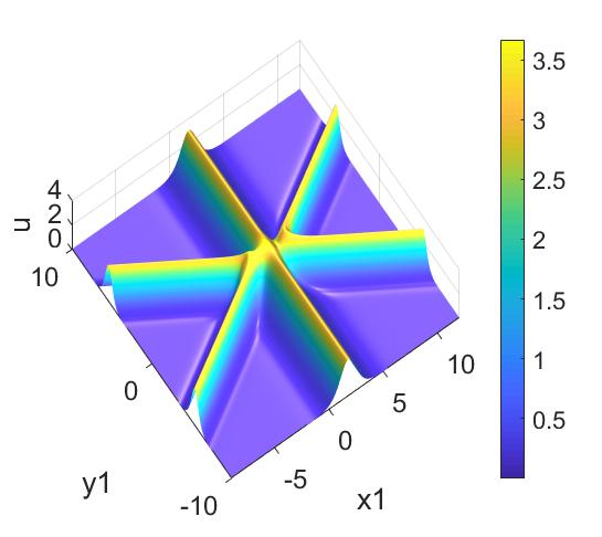
2.2 A hybrid of a V-type soliton and breathers

Refer to caption
(a) t=0
Refer to caption
(b) t=0
Figure 2: A hybrid of a V-type soliton and one breather of the 4D Fokas equation with parameters N=2,p1=12+i,p2=12i,δij=1(i,j=1,2),x2=0,y2=0N=2,p_{1}=\frac{1}{2}+i,p_{2}=\frac{1}{2}-i,\delta_{ij}=1\,(i,j=1,2),x_{2}=0,y_{2}=0, and t=0t=0 in (8). Panel (b) is the contour plot of panel (a).

In addition to the soliton solutions, equation (1) admits a hybrid of V-type soliton and breather solutions, assuming N2N\geq 2 and δij=1\delta_{ij}=1 and some parameters pip_{i} are complex in equation (8). We first consider the case of N=2N=2 and δij=1\delta_{ij}=1. The following parameters are further taken in equation (8):

p1=12+i,p2=12i,δ12=1,δ21=1,p_{1}=\frac{1}{2}+i,\quad p_{2}=\frac{1}{2}-i,\quad\delta_{12}=1,\quad\delta_{21}=1,

and the mixed solution consisting of a V-type soliton and one breather solution is derived, see Fig. 2. For this mixed solution the expression of ff is as follows:

f=\displaystyle f= cosh[γ123(y1+y2)]+sinh[γ123(y1+y2)]+cosh[γ1+23(y1+y2)]\displaystyle\cosh[\gamma_{1}-2\sqrt{3}(y_{1}+y_{2})]+\sinh[\gamma_{1}-2\sqrt{3}(y_{1}+y_{2})]+\cosh[\gamma_{1}+2\sqrt{3}(y_{1}+y_{2})] (16)
+sinh[γ123(y1+y2)]+45[cosh(2γ1)+sinh(2γ1)]45[cosh(γ1)\displaystyle+\sinh[\gamma_{1}-2\sqrt{3}(y_{1}+y_{2})]+\frac{4}{5}[\cosh(2\gamma_{1})+\sinh(2\gamma_{1})]-\frac{4}{5}[\cosh(\gamma_{1})
+sinh(γ1)]sin(γ2)25[cosh(γ1)+sinh(γ1)]cos(γ2),\displaystyle+\sinh(\gamma_{1})]\sin(\gamma_{2})-\frac{2}{5}[\cosh(\gamma_{1})+\sinh(\gamma_{1})]\cos(\gamma_{2}),

where

γ1=x1+2x2+332t,γ2=2x1+4x2+3t.\displaystyle\gamma_{1}=x_{1}+2x_{2}+\frac{33}{2}t,\quad\gamma_{2}=2x_{1}+4x_{2}+3t. (17)

Furthermore, for larger NN, we can derive the mixed solution consisting of a V-type soliton and more breathers. For example, when we take the parameters N=3,p1=12+i,p2=12i,p3=23N=3,p_{1}=\frac{1}{2}+i,p_{2}=\frac{1}{2}-i,p_{3}=\frac{2}{3} and δij=1(i,j=1,2,3)\delta_{ij}=1\,(i,j=1,2,3) in equation (8) the mixed solution consisting of a V-type soliton and two breathers is presented in Fig. 3.

Refer to caption
(a) t=0
Refer to caption
(b) t=0
Figure 3: A hybrid of a V-type soliton and two breathers of the 4D Fokas equation with parameters N=3,p1=12+i,p2=12i,p3=23,δij=1(i,j=1,2,3),x2=0,y2=0N=3,p_{1}=\frac{1}{2}+i,p_{2}=\frac{1}{2}-i,p_{3}=\frac{2}{3},\delta_{ij}=1\,(i,j=1,2,3),x_{2}=0,y_{2}=0, and t=0t=0 in (8). Panel (b) is the contour plot of panel (a).

3 Rational solutions in the determinant form

The rational solutions of low-dimensional integrable systems have been extensively investigated. However, there are few studies of rational solutions in high-dimensional systems. Inspired by the works of Ohta and Yang yo1 ; yo2 ; yo3 , the rational solutions of the 4D\rm 4D Fokas equation are constructed by introducing the following Lemma.

Lemma 2. The bilinear equation of KP hierarchy (7) has solutions

τn=det1i,jN(M2i1,2j1(n)),\displaystyle\tau^{{}^{\prime}}_{n}=\det_{1\leq i,j\leq N}(M^{(n)}_{2i-1,2j-1}), (18)

with the matrix element Mi,j(n)M^{(n)}_{i,j} satisfying the following differential and difference relations

z1Mi,j(n)=Φi(n)Ψj(n),\displaystyle\partial_{z_{1}}M^{(n)}_{i,j}=\Phi^{(n)}_{i}\Psi^{(n)}_{j}, (19)
mi,j(n+1)=Mi,j(n)+Φi(n)Ψj(n+1),\displaystyle m^{(n+1)}_{i,j}=M^{(n)}_{i,j}+\Phi^{(n)}_{i}\Psi^{(n+1)}_{j},
z2Mi,j(n)=Φi(n+1)Ψj(n)+Φi(n)Ψj(n1),\displaystyle\partial_{z_{2}}M^{(n)}_{i,j}=\Phi^{(n+1)}_{i}\Psi^{(n)}_{j}+\Phi^{(n)}_{i}\Psi^{(n-1)}_{j},
z3Mi,j(n)=Φi(n+2)Ψj(n)+Φi(n+1)Ψj(n1)+Φi(n)Ψj(n2),\displaystyle\partial_{z_{3}}M^{(n)}_{i,j}=\Phi^{(n+2)}_{i}\Psi^{(n)}_{j}+\Phi^{(n+1)}_{i}\Psi^{(n-1)}_{j}+\Phi^{(n)}_{i}\Psi^{(n-2)}_{j},
zkΦ=Φi(n+k),zkΨi=Ψi(nk),(k=1,2,3).\displaystyle\partial_{z_{k}}\Phi=\Phi^{(n+k)}_{i},\quad\partial_{z_{k}}\Psi_{i}=-\Psi^{(n-k)}_{i},(k=1,2,3).

Here Mi,j(n)M^{(n)}_{i,j}, Φi(n)\Phi^{(n)}_{i}, and Ψj(n)\Psi^{(n)}_{j} are functions of the variables z1,z2z_{1},z_{2}, and z3z_{3}. The above relations were proven in yo1 , hence we omit here the proof. The functions Φi(n)\Phi_{i}^{(n)}, Ψj(n)\Psi_{j}^{(n)}, and Mij(n)M_{ij}^{(n)} are defined by

Φi(n)\displaystyle\Phi_{i}^{(n)} =Aipneξ,Ψj(n)=Bj(q)eη,\displaystyle=A_{i}p^{n}e^{\xi},\quad\Psi_{j}^{(n)}=B_{j}(-q)e^{\eta}, (20)
Mi,j(n)\displaystyle M^{(n)}_{i,j} =z1Φi(n)Ψj(n)𝑑z1=AiBj1p+q(pq)neξ+η,\displaystyle=\int^{z_{1}}\Phi_{i}^{(n)}\Psi_{j}^{(n)}dz_{1}=A_{i}B_{j}\frac{1}{p+q}(-\frac{p}{q})^{n}e^{\xi+\eta},

where

Ai=\displaystyle A_{i}= k=0ick(ik)!(pp)ik,Bj=l=0jdl(jl)!(qq)jl,\displaystyle\sum_{k=0}^{i}\frac{c_{k}}{(i-k)!}(p\partial_{p})^{i-k},\quad B_{j}=\sum_{l=0}^{j}\frac{d_{l}}{(j-l)!}(q\partial_{q})^{j-l}, (21)
ξ=\displaystyle\xi= pz1+p2z2+p3z3+ξ0,η=qz1q2z2+q3z3+η0.\displaystyle pz_{1}+p^{2}z_{2}+p^{3}z_{3}+\xi_{0},\quad\eta=qz_{1}-q^{2}z_{2}+q^{3}z_{3}+\eta_{0}.

For simplicity, we can rewrite the functions Mi,j(n)M^{(n)}_{i,j} as

Mi,j(n)\displaystyle M^{(n)}_{i,j} =k=0ick(ik)!(pp+ξ+n)ik\displaystyle=\sum_{k=0}^{i}\frac{c_{k}}{(i-k)!}(p\partial_{p}+\xi^{{}^{\prime}}+n)^{i-k} (22)
×\displaystyle\times l=0jdl(jl)!(qq+ηn)jl1p+q,\displaystyle\sum_{l=0}^{j}\frac{d_{l}}{(j-l)!}(q\partial_{q}+\eta^{{}^{\prime}}-n)^{j-l}\frac{1}{p+q},

where

ξ=\displaystyle\xi^{{}^{\prime}}= pz1+2p2z2+3p3z3,η=qz12q2z2+3q3z3,\displaystyle pz_{1}+2p^{2}z_{2}+3p^{3}z_{3},\quad\eta^{{}^{\prime}}=qz_{1}-2q^{2}z_{2}+3q^{3}z_{3}, (23)

and pp, qq, ckc_{k}, and dld_{l} are arbitrary complex constants. Further, taking the parameter constraints

p=q=1,ck=dk,p=q=1,\qquad c_{k}=d^{*}_{k},

setting τ0=f\tau^{{}^{\prime}}_{0}=f, z1=k1x1+k2x2z_{1}=k_{1}x_{1}+k_{2}x_{2}, z2=k1k2(k22k12)2k3k4i(k3y1+k4y2)z_{2}=\sqrt{\frac{{k_{1}k_{2}}(k^{2}_{2}-k^{2}_{1})}{2k_{3}k_{4}}}i(k_{3}y_{1}+k_{4}y_{2}), and z3=2k2(k22k12)tz_{3}=-2k_{2}(k^{2}_{2}-k^{2}_{1})t, the rational solutions of the 4D Fokas equation can be generated from equation (7). Based on the above results, the rational solutions of the 4D Fokas equation are presented in the following Theorem.

Theorem 2. The (4+1)(4+1)-dimensional Fokas equation (1) has rational solutions

u=(k22k12)(lnf)xx,x=k1x1+k2x2,\displaystyle u=(k^{2}_{2}-k^{2}_{1})(\ln f)_{xx},\quad x=k_{1}x_{1}+k_{2}x_{2}, (24)

where

f=det1i,jN(M2i1,2j1(n))n=0.\displaystyle f=\det\limits_{1\leq i,j\leq N}(M^{(n)}_{2i-1,2j-1})\mid_{n=0}. (25)

The matrix elements in ff are defined by

Mi,j(n)\displaystyle M_{i,j}^{(n)} =k=0ick(ik)!(pp+ξ+n)ik\displaystyle=\sum_{k=0}^{i}\frac{c_{k}}{(i-k)!}(p\partial_{p}+\xi^{{}^{\prime}}+n)^{i-k} (26)
×l=0jcl(jl)!(pp+ξn)jl1p+pp=1,\displaystyle\times\sum_{l=0}^{j}\frac{c_{l}^{*}}{(j-l)!}(p^{*}\partial_{p^{*}}+\xi^{{}^{\prime}*}-n)^{j-l}\frac{1}{p+p^{*}}\mid_{p=1},
ξ\displaystyle\xi^{{}^{\prime}} =k1x1+k2x2+2k1k2k3(k22k12)k4y1\displaystyle=k_{1}x_{1}+k_{2}x_{2}+\sqrt{\frac{{2k_{1}k_{2}k_{3}}(k^{2}_{2}-k^{2}_{1})}{-k_{4}}}y_{1}
+2k1k2k4(k22k12)k3y23k2(k22k12)t,\displaystyle+\sqrt{\frac{{2k_{1}k_{2}k_{4}}(k^{2}_{2}-k^{2}_{1})}{-k_{3}}}y_{2}-3k_{2}(k^{2}_{2}-k^{2}_{1})t,

the asterisk denotes the complex conjugation, i,j,ki,j,k, and ll are arbitrary positive integers, and ckc_{k} and clc_{l} are arbitrary complex constants. We take k1=1,k2=65,k3=1k_{1}=1,k_{2}=\frac{6}{5},k_{3}=1, and k4=1k_{4}=1 in this section.

3.1 Fundamental rational solution

According to Theorem 2, taking the parameters N=1N=1, c0=1c_{0}=1, and c1=0c_{1}=0 in equation (24), we first derive the fundamental rational solution of the 4D Fokas equation:

u=2(k12k22)k3k42k1k2(k12k22)[k3y1+k4y2]2+k3k4llump214k3k4(18k1k2(k22k12)[k3y1+k4y2]2+9k3k4llump2+94k3k4)2,\displaystyle u=2(k^{2}_{1}-k^{2}_{2})k_{3}k_{4}\frac{2k_{1}k_{2}(k^{2}_{1}-k^{2}_{2})[k_{3}y_{1}+k_{4}y_{2}]^{2}+k_{3}k_{4}l_{lump}^{2}-\frac{1}{4}k_{3}k_{4}}{\left(18k_{1}k_{2}(k^{2}_{2}-k^{2}_{1})[k_{3}y_{1}+k_{4}y_{2}]^{2}+9k_{3}k_{4}l_{lump}^{2}+\frac{9}{4}k_{3}k_{4}\right)^{2}}, (27)

where

llump=k1x1+k2x2+3(k12k2k23)t+12.\displaystyle l_{lump}=k_{1}x_{1}+k_{2}x_{2}+3(k^{2}_{1}k_{2}-k^{3}_{2})t+\frac{1}{2}. (28)

As can be seen from the above expressions, in order to ensure that the fundamental rational solution is non-singular, k1k2k3k4(k22k12)>0k_{1}k_{2}k_{3}k_{4}(k_{2}^{2}-k_{1}^{2})>0 must be held. The fundamental rational solution is a lump and has the following extreme points in the (x1,y1)(x_{1},y_{1})-plane, see Fig. 4:

Λ1\displaystyle\Lambda_{1} =(x11,y11)=(k2k1x2+3(k23k1k1k2)t+12k1,y1=k4k3y2),\displaystyle=(x_{11},y_{11})=\left(-\frac{k_{2}}{k_{1}}x_{2}+3(\frac{k^{3}_{2}}{k_{1}}-k_{1}k_{2})t+\frac{1}{2k_{1}},y1=-\frac{k_{4}}{k_{3}}y_{2}\right),
Λ2\displaystyle\Lambda_{2} =(x12,y12)=(k2k1x2+3(k23k1k1k2)t+1+32k1,y1=k4k3y2),\displaystyle=(x_{12},y_{12})=\left(-\frac{k_{2}}{k_{1}}x_{2}+3(\frac{k^{3}_{2}}{k_{1}}-k_{1}k_{2})t+\frac{1+\sqrt{3}}{2k_{1}},y1=-\frac{k_{4}}{k_{3}}y_{2}\right),
Λ3\displaystyle\Lambda_{3} =(x13,y13)=(k2k1x2+3(k23k1k1k2)t+132k1,y1=k4k3y2).\displaystyle=(x_{13},y_{13})=\left(-\frac{k_{2}}{k_{1}}x_{2}+3(\frac{k^{3}_{2}}{k_{1}}-k_{1}k_{2})t+\frac{1-\sqrt{3}}{2k_{1}},y1=-\frac{k_{4}}{k_{3}}y_{2}\right){\color[rgb]{1,0,0}.}

After simple calculations, we get a maximum value HMax=H(x11,y11)=8(k22k12)H_{Max}=H(x_{11},y_{11})=8(k^{2}_{2}-k^{2}_{1}) and two minimum values HMin=H(x12,y12)=H(x13,y13)=k12k22H_{Min}=H(x_{12},y_{12})=H(x_{13},y_{13})=k^{2}_{1}-k^{2}_{2} of the lump solution. The lump trajectory is k1x1+k2x2+3(k12k2k23)t+12=0k_{1}x_{1}+k_{2}x_{2}+3(k^{2}_{1}k_{2}-k^{3}_{2})t+\frac{1}{2}=0.

Refer to caption
(a) t=0
Refer to caption
(b) t=0
Figure 4: First-order rational solution for the 4D Fokas equation in the (x1,y1)(x_{1},y_{1})-plane with parameters N=1,c0=1,c1=0,k1=1,k2=65,k3=1,k4=1,x2=0,y2=0N=1,c_{0}=1,c_{1}=0,k_{1}=1,k_{2}=\frac{6}{5},k_{3}=1,k_{4}=1,x_{2}=0,y_{2}=0, and t=0t=0 in equation (24). Panel (b) is the contour plot of panel (a).

3.2 High-order rational solutions

Refer to caption
(a) t=0
Refer to caption
(b) t=0
Refer to caption
(c) t=0
Refer to caption
(d) t=0
Figure 5: Second-order rational solutions of the 4D Fokas equation with parameters N=2,c1=0,c2=0,k1=1,k2=65,k3=1,k4=1,x2=0,y2=0N=2,c_{1}=0,c_{2}=0,k_{1}=1,k_{2}=\frac{6}{5},k_{3}=1,k_{4}=1,x_{2}=0,y_{2}=0, and t=0t=0 in equation (24). (a): a fundamental pattern with c0=1c_{0}=1 and c3=112c_{3}=-\frac{1}{12}; (b): a triangular pattern with c0=1c_{0}=1 and c3=30c_{3}=-30. Panels (c) and (d) are the contour plots of panels (a) and (b), respectively.

In this section, we consider the high-order rational solutions of the 4D Fokas equation. NN-order lump solutions are derived in the (x1,y1)(x_{1},y_{1})-plane from Theorem 2 for any given NN. For example, taking N=2,k1=1,k2=65,k3=1N=2,k_{1}=1,k_{2}=\frac{6}{5},k_{3}=1, and k4=1k_{4}=1, the second-order lump solutions u2ordu_{\rm 2ord} are obtained

u2ord=(k22k12)(ln|M11(0)M13(0)M31(0)M33(0)|)xx,u_{\rm 2ord}=(k_{2}^{2}-k^{2}_{1})\left(\ln\begin{vmatrix}M^{(0)}_{11}&M^{(0)}_{13}\\ M^{(0)}_{31}&M^{(0)}_{33}\end{vmatrix}\right)_{xx}, (29)

where Mi,j(n)M_{i,j}^{(n)} are defined in Theorem 2. As shown in Fig. 5, the second-order lumps have two types of patterns, which are controlled by four free parameters. Similarly, the third-order lump solutions are derived by taking N=3,k1=1,k2=65,k3=1N=3,k_{1}=1,k_{2}=\frac{6}{5},k_{3}=1, and k4=1k_{4}=1. The third-order lumps have three types of patterns, which are controlled by six parameters, see Fig. 6. For larger values of NN, as more free parameters will be generated, the patterns of the lumps will be more abundant and their dynamic behavior will be more complicated. We note that the pattern dynamics of high-order lumps is similar to rogue waves dynamics in (1+1)(1+1)-dimensional systems.

Refer to caption
(a) t=0
Refer to caption
(b) t=0
Refer to caption
(c) t=0
Refer to caption
(d) t=0
Refer to caption
(e) t=0
Refer to caption
(f) t=0
Figure 6: Third-order rational solutions of the 4D Fokas equation with parameters N=3,c1=0,c2=0,c4=0,k1=1,k2=65,k3=1,k4=1,x2=0,y2=0N=3,c_{1}=0,c_{2}=0,c_{4}=0,k_{1}=1,k_{2}=\frac{6}{5},k_{3}=1,k_{4}=1,x_{2}=0,y_{2}=0, and t=0t=0 in equation (24). (a): a fundamental pattern with c0=1,c3=112c_{0}=1,c_{3}=-\frac{1}{12} and c3=1240c_{3}=-\frac{1}{240}; (b): a triangular pattern with c0=1,c3=253c_{0}=1,c_{3}=-\frac{25}{3} and c5=0c_{5}=0; (c): a ring pattern with c0=1,c3=0c_{0}=1,c_{3}=0 and c5=20c_{5}=20. Panels (d), (e), and (f) are the contour plots of panels (a), (b), and (c), respectively.

4 Semi-rational solutions in the determinant form

In this section, we present a Theorem for constructing the semi-rational solutions of the 4D Fokas equation. In order to obtain the semi-rational solutions of the 4D Fokas equation, we will first introduce the following differential operators

Ξi=k=0niaik(pipi)nik,j=l=0njajl(pjpj)njl.\displaystyle\Xi_{i}=\sum_{k=0}^{n_{i}}a_{ik}(p_{i}\partial_{p_{i}})^{n_{i}-k},\quad\mho_{j}=\sum_{l=0}^{n_{j}}a^{*}_{jl}(p^{*}_{j}\partial_{p^{*}_{j}})^{n_{j}-l}. (30)

We choose the following functions

φi(n)=Ξipineξi,\displaystyle\varphi^{(n)}_{i}=\Xi_{i}p^{n}_{i}e^{\xi^{i}}, (31)
ψj(n)=j(qj)neηj,\displaystyle\psi^{(n)}_{j}=\mho_{j}(-q_{j})^{-n}e^{\eta_{j}},
Ki,j(n)=Ξij1pi+pj[δij+(pipj)neξi+ξj].\displaystyle K^{(n)}_{i,j}=\Xi_{i}\mho_{j}\frac{1}{p_{i}+p^{*}_{j}}[\delta_{ij}+(-\frac{p_{i}}{p^{*}_{j}})^{n}e^{\xi_{i}+\xi^{*}_{j}}].

The functions φi(n)\varphi^{(n)}_{i} and ψj(n)\psi^{(n)}_{j} also satisfy the equation (11). For simplicity, we rewrite the matrix element Ki,j(n)K^{(n)}_{i,j} as

Ki,j(n)\displaystyle K_{i,j}^{(n)} =(pipj)eξi+ξjk=0niaik(pipi+ξi+n)nik\displaystyle=(-\frac{p_{i}}{p^{*}_{j}})e^{\xi_{i}+\xi^{*}_{j}}\sum_{k=0}^{n_{i}}a_{ik}(p_{i}\partial_{p_{i}}+\xi^{{}^{\prime}}_{i}+n)^{n_{i}-k} (32)
×l=0njajl(pjpj+ξjn)njl1pi+pj+δijainiajnj,\displaystyle\times\sum_{l=0}^{n_{j}}a_{jl}^{*}(p^{*}_{j}\partial_{p^{*}_{j}}+\xi^{{}^{\prime}*}_{j}-n)^{n_{j}-l}\frac{1}{p_{i}+p^{*}_{j}}+\delta_{ij}a_{in_{i}}a_{jn_{j}}^{*},

where

ξi\displaystyle\xi_{i} =piz1+pi2z2+pi3z3+ξi0,\displaystyle=p_{i}z_{1}+p_{i}^{2}z_{2}+p_{i}^{3}z_{3}+\xi_{i0}, (33)
ξi\displaystyle\xi^{{}^{\prime}}_{i} =piz1+2pi2z2+3pi3z3.\displaystyle=p_{i}z_{1}+2p_{i}^{2}z_{2}+3p_{i}^{3}z_{3}.

Here pip_{i} and aika_{ik} are arbitrary complex constants, δij=0,1\delta_{ij}=0,1, and nin_{i} are arbitrary positive integers. Furthermore, taking τ0=f\tau_{0}=f, z1=k1x1+k2x2z_{1}=k_{1}x_{1}+k_{2}x_{2}, z2=k1k2(k22k12)2k3k4i(k3y1+k4y2)z_{2}=\sqrt{\frac{{k_{1}k_{2}}(k^{2}_{2}-k^{2}_{1})}{2k_{3}k_{4}}}i(k_{3}y_{1}+k_{4}y_{2}), and z3=2k2(k22k12)tz_{3}=-2k_{2}(k^{2}_{2}-k^{2}_{1})t, then, the semi-rational solutions of the 4D Fokas equation would be derived. Thus, semi-rational solutions of 4D Fokas equation can be determined by the following Theorem.

Theorem 3. The (4+1)(4+1)-dimensional Fokas equation (1) has semi-rational solutions

u=(k22k12)(lnf)xx,x=k1x1+k2x2,\displaystyle u=(k^{2}_{2}-k^{2}_{1})(\ln f)_{xx},\quad x=k_{1}x_{1}+k_{2}x_{2}, (34)

where

f=det1i,jN(Ki,j(n))n=0,\displaystyle f=\det\limits_{1\leq i,j\leq N}(K^{(n)}_{i,j})\mid_{n=0}, (35)

and the matrix elements in ff are defined by

Ki,j(n)\displaystyle K_{i,j}^{(n)} =(pipj)eξi+ξjk=0nicik(pipi+ξi+n)nik\displaystyle=(-\frac{p_{i}}{p^{*}_{j}})e^{\xi_{i}+\xi^{*}_{j}}\sum_{k=0}^{n_{i}}c_{ik}(p_{i}\partial_{p_{i}}+\xi^{{}^{\prime}}_{i}+n)^{n_{i}-k} (36)
×\displaystyle\times l=0njcjl(pjpj+ξjn)njl1pi+pj+δijainiajnj,\displaystyle\sum_{l=0}^{n_{j}}c_{jl}^{*}(p^{*}_{j}\partial_{p^{*}_{j}}+\xi^{{}^{\prime}*}_{j}-n)^{n_{j}-l}\frac{1}{p_{i}+p^{*}_{j}}+\delta_{ij}a_{in_{i}}a_{jn_{j}}^{*},
ξi\displaystyle\xi_{i} =k1pix1+k2pix2+k1k2k3(k22k12)2k4pi2y1\displaystyle=k_{1}p_{i}x_{1}+k_{2}p_{i}x_{2}+\sqrt{\frac{{k_{1}k_{2}k_{3}}(k^{2}_{2}-k^{2}_{1})}{-2k_{4}}}p_{i}^{2}y_{1}
+k1k2k4(k22k12)2k3pi2y2k2(k22k12)pi3t+ξi0,\displaystyle+\sqrt{\frac{{k_{1}k_{2}k_{4}}(k^{2}_{2}-k^{2}_{1})}{-2k_{3}}}p_{i}^{2}y_{2}-k_{2}(k^{2}_{2}-k^{2}_{1})p_{i}^{3}t+\xi_{i0},
ξi\displaystyle\xi^{{}^{\prime}}_{i} =k1pix1+k2pix2+2k1k2k3(k22k12)k4pi2y1\displaystyle=k_{1}p_{i}x_{1}+k_{2}p_{i}x_{2}+\sqrt{\frac{{2k_{1}k_{2}k_{3}}(k^{2}_{2}-k^{2}_{1})}{-k_{4}}}p^{2}_{i}y_{1}
+2k1k2k4(k22k12)k3pi2y23k2(k22k12)pi3t.\displaystyle+\sqrt{\frac{{2k_{1}k_{2}k_{4}}(k^{2}_{2}-k^{2}_{1})}{-k_{3}}}p^{2}_{i}y_{2}-3k_{2}(k^{2}_{2}-k^{2}_{1})p^{3}_{i}t.

The asterisk denotes the complex conjugation, i,j,ki,j,k, and ll are arbitrary positive integers, and k1k_{1}, k2k_{2}, k3k_{3}, and k4k_{4} are arbitrary real constants. It is not difficult to find that the semi-rational solutions will become rational solutions when δij=0\delta_{ij}=0. We note that the patterns of rational solutions are similar to those corresponding to rational solutions of the Davey-Stewartson equation, reported in Refs. rao1 ; rao2 ; qc .

4.1 Lumps on one-soliton background

The semi-rational solution ulsu_{\rm ls} consisting of a lump and a soliton is derived by taking N=1,ni=1,a01=0,a11=1,p1=1,δii=1N=1,n_{i}=1,a_{01}=0,a_{11}=1,p_{1}=1,\delta_{ii}=1, and δij=0(ij)\delta_{ij}=0\,(i\neq j) in equation (34). The expression of ulsu_{\rm ls} is as follows

uls=2(k12k22)k3k4{[2k1k2(k12k22)l12+k3k4llump214k3k4]eξ4k3k4(llump+1)2+8k1k2(k12k22)l12+k3k4}eξ([18k1k2(k22k12)l12+9k3k4llump2+94k3k4]eξ+18k3k4)2,\displaystyle u_{\rm ls}=2(k^{2}_{1}-k^{2}_{2})k_{3}k_{4}\frac{\begin{Bmatrix}&[2k_{1}k_{2}(k^{2}_{1}-k^{2}_{2})l_{1}^{2}+k_{3}k_{4}l_{lump}^{2}-\frac{1}{4}k_{3}k_{4}]e^{\xi}\\ &-4k_{3}k_{4}(l_{lump}+1)^{2}+8k_{1}k_{2}(k^{2}_{1}-k^{2}_{2})l_{1}^{2}+k_{3}k_{4}\end{Bmatrix}e^{\xi}}{\left([18k_{1}k_{2}(k^{2}_{2}-k^{2}_{1})l_{1}^{2}+9k_{3}k_{4}l_{lump}^{2}+\frac{9}{4}k_{3}k_{4}]e^{\xi}+18k_{3}k_{4}\right)^{2}}, (37)

where

l1=k3y1+k4y2,ξ=2k1x1+2k2x2+2(k12k2k23)t,l_{1}=k_{3}y_{1}+k_{4}y_{2},\quad\xi=2k_{1}x_{1}+2k_{2}x_{2}+2(k_{1}^{2}k_{2}-k_{2}^{3})t,
llump=k1x1+k2x2+3(k12k2k23)t.l_{lump}=k_{1}x_{1}+k_{2}x_{2}+3(k^{2}_{1}k_{2}-k^{3}_{2})t.

By choosing different parameters k1,k2,k3k_{1},k_{2},k_{3}. and k4k_{4}, we derive a lump fusing into or fissioning from a dark soliton or from a bright soliton, see Fig. 7. The classification of four different types of interaction between lumps and one-soliton solutions is given in Table 1. From the above results, we can easily calculate that the velocities of lump and soliton are Vlump=3k12k2k23k1V_{\rm lump}=3\frac{k^{2}_{1}k_{2}-k^{3}_{2}}{k_{1}} and Vsoliton=k12k2k23k1V_{\rm soliton}=\frac{k^{2}_{1}k_{2}-k^{3}_{2}}{k_{1}}, respectively. The velocity of lump is always greater than that of soliton, see Fig. 7.

Refer to caption
(a) t=-5
Refer to caption
(b) t=0
Refer to caption
(c) t=5
Refer to caption
(d) t=-5
Refer to caption
(e) t=0
Refer to caption
(f) t=5
Refer to caption
(g) t=-5
Refer to caption
(h) t=0
Refer to caption
(i) t=5
Refer to caption
(j) t=-5
Refer to caption
(k) t=0
Refer to caption
(l) t=5
Figure 7: Time evolution of semi-rational solution ulsu_{\rm ls} of the 4D Fokas equation, (a,b,c): A bright lump is annihilated by a bright soliton with parameters k1=1,k2=1.2,k3=1,k4=1,x2=0k_{1}=-1,k_{2}=-1.2,k_{3}=1,k_{4}=1,x_{2}=0, and y2=0y_{2}=0; (d,e,f): A bright lump is created from a bright soliton with parameters k1=1,k2=1.2,k3=1,k4=1,x2=0k_{1}=1,k_{2}=-1.2,k_{3}=1,k_{4}=1,x_{2}=0, and y2=0y_{2}=0; (g,h,i): A dark lump is annihilated by a dark soliton with parameters k1=1.2,k2=1,k3=1,k4=1,x2=0k_{1}=-1.2,k_{2}=1,k_{3}=1,k_{4}=-1,x_{2}=0, and y2=0y_{2}=0; (j,k,l): A dark lump is created from a dark soliton with parameters k1=1.2,k2=1,k3=1,k4=1,x2=0k_{1}=-1.2,k_{2}=-1,k_{3}=1,k_{4}=-1,x_{2}=0, and y2=0y_{2}=0.
Parameter condition (i)    Parameter condition (ii)     Results
k3k4>0k_{3}k_{4}>0    k2<k1<0k_{2}<k_{1}<0     a lump is annihilated
k3k4<0k_{3}k_{4}<0    |k2|>k1>0>k2|k_{2}|>k_{1}>0>k_{2}     by a bright soliton
k3k4>0k_{3}k_{4}>0    k2>k1>0k_{2}>k_{1}>0     a lump is created
k3k4<0k_{3}k_{4}<0    k2>|k1|>0>k1k_{2}>|k_{1}|>0>k_{1}     from a bright soliton
k3k4>0k_{3}k_{4}>0    |k1|>k2>0>k1|k_{1}|>k_{2}>0>k_{1}     a lump is annihilated
k3k4<0k_{3}k_{4}<0    k1>k2>0k_{1}>k_{2}>0     by a dark soliton
k3k4>0k_{3}k_{4}>0    k1>|k2|>0>k2k_{1}>|k_{2}|>0>k_{2}     a lump is created
k3k4<0k_{3}k_{4}<0    k1<k2<0k_{1}<k_{2}<0     from a dark soliton
Table 1: Classification of four different types of interactions between lumps and one-soliton solution.
Refer to caption
(a) t=-7
Refer to caption
(b) t=-1
Refer to caption
(c) t=1
Refer to caption
(d) t=7
Figure 8: Time evolution of the process of fission of two lumps from a bright soliton of the 4D Fokas equation with parameters N=1,ni=2,a01=0,a11=4,a12=1,p1=1,δii=1,δ12=0,k1=1,k2=1.2,k3=1,k4=1,x2=0N=1,n_{i}=2,a_{01}=0,a_{11}=4,a_{12}=1,p_{1}=1,\delta_{ii}=1,\delta_{12}=0,k_{1}=1,k_{2}=1.2,k_{3}=1,k_{4}=1,x_{2}=0, and y2=0y_{2}=0 in equation (34).

The semi-rational solutions consisting of more lumps and a soliton are generated for N=1N=1 and ni2n_{i}\geq 2 in equation (34). For example, taking N=1,ni=2,a01=0,a11=4,a12=1,p1=1,δ11=1N=1,n_{i}=2,a_{01}=0,a_{11}=4,a_{12}=1,p_{1}=1,\delta_{11}=1, and δ12=0\delta_{12}=0 in equation (34), we can derive the semi-rational solutions composed of two lumps and a soliton. There are also four distinct types of such semi-rational solutions. To have an idea of the dynamics of such semi-rational solutions, we show here only the process of fission of two lumps from a bright soliton, see Fig. 8.

4.2 Lumps on multi-solitons background

For N2,ni=1,δ11=1,δ12=0,δ21=0N\geq 2,n_{i}=1,\delta_{11}=1,\delta_{12}=0,\delta_{21}=0, and δ22=1\delta_{22}=1 in equation (34), the semi-rational solutions consisting of more lumps and more solitons are derived. For example, taking N=1,ni=2,k1=1,k2=2,k3=1,k4=1,a10=1,a20=1,a11=1,a21=1,p1=12,p2=13,δ11=1,δ12=0,δ21=0N=1,n_{i}=2,k_{1}=1,k_{2}=2,k_{3}=1,k_{4}=1,a_{10}=1,a_{20}=1,a_{11}=1,a_{21}=1,p_{1}=\frac{1}{2},p_{2}=\frac{1}{3},\delta_{11}=1,\delta_{12}=0,\delta_{21}=0, and δ22=1\delta_{22}=1 in equation (34), we obtain the interaction of local wave structures described by two lumps and two solitons. The exact expression of the corresponding solution u2lsu_{2ls} is as follows

u2ls=(k22k12)(ln|K11(0)K12(0)K21(0)K22(0)|)xx,\displaystyle u_{\rm 2ls}=(k_{2}^{2}-k^{2}_{1})\left(\ln\begin{vmatrix}K^{(0)}_{11}&K^{(0)}_{12}\\ K^{(0)}_{21}&K^{(0)}_{22}\end{vmatrix}\right)_{xx}, (38)

where

K11(0)=1+(34(y1+y2)2+14(x1+2x292t+1)2+14)ex1+2x232t,K^{(0)}_{11}=1+\left(\frac{3}{4}(y_{1}+y_{2})^{2}+\frac{1}{4}(x_{1}+2x_{2}-\frac{9}{2}t+1)^{2}+\frac{1}{4}\right)e^{x_{1}+2x_{2}-\frac{3}{2}t},
K12(0)=(2(y1+y2)25+15(x1+2x2134t+1310)2516(t+25)2+36125+A)eϱ1,K^{(0)}_{12}=\left(\frac{2(y_{1}+y_{2})^{2}}{5}+\frac{1}{5}(x_{1}+2x_{2}-\frac{13}{4}t+\frac{13}{10})^{2}-\frac{5}{16}(t+\frac{2}{5})^{2}+\frac{36}{125}+A\right)e^{\varrho_{1}},
K21(0)=(2(y1+y2)25+15(x1+2x2134t+1310)2516(t+25)2+36125A)eϱ2,K^{(0)}_{21}=\left(\frac{2(y_{1}+y_{2})^{2}}{5}+\frac{1}{5}(x_{1}+2x_{2}-\frac{13}{4}t+\frac{13}{10})^{2}-\frac{5}{16}(t+\frac{2}{5})^{2}+\frac{36}{125}-A\right)e^{\varrho_{2}},
K22(0)=1+(29(y1+y2)2+6(x1+2x22t+32)2+38)e23x1+43x249t,K^{(0)}_{22}=1+\left(\frac{2}{9}(y_{1}+y_{2})^{2}+6(x_{1}+2x_{2}-2t+\frac{3}{2})^{2}+\frac{3}{8}\right)e^{\frac{2}{3}x_{1}+\frac{4}{3}x_{2}-\frac{4}{9}t},
A=3(y1+y2)(13x1+23x2+t+915),A=\sqrt{-3}(y_{1}+y_{2})(\frac{1}{3}x_{1}+\frac{2}{3}x_{2}+t+\frac{9}{15}),
ϱ1=56x1+53x23536t+5336(y1+y2),\varrho_{1}=\frac{5}{6}x_{1}+\frac{5}{3}x_{2}-\frac{35}{36}t+\frac{5\sqrt{-3}}{36}(y_{1}+y_{2}),
ϱ2=56x1+53x23536t5336(y1+y2).\varrho_{2}=\frac{5}{6}x_{1}+\frac{5}{3}x_{2}-\frac{35}{36}t-\frac{5\sqrt{-3}}{36}(y_{1}+y_{2}).

The five panels in Fig. 9 describe the process of creation of two lumps from the background of two solitons. As shown in Fig. 9, with time evolution more peaks are created during the interaction between lumps and solitons around t=2.5t=2.5, then two lumps and two solitons are completely separated around t=10t=10.

Refer to caption
(a) t=-10
Refer to caption
(b) t=-2
Refer to caption
(c) t=0
Refer to caption
(d) t=2
Refer to caption
(e) t=10
Figure 9: The time evolution of fission of two lumps from two solitons for the 4D Fokas equation with parameters N=1,ni=2,a10=1,a20=1,a11=1,a21=1,p1=12,p2=13,δ11=1,δ12=0,δ21=0,δ22=1,k1=1,k2=2,k3=1,k4=1,x2=0N=1,n_{i}=2,a_{10}=1,a_{20}=1,a_{11}=1,a_{21}=1,p_{1}=\frac{1}{2},p_{2}=\frac{1}{3},\delta_{11}=1,\delta_{12}=0,\delta_{21}=0,\delta_{22}=1,k_{1}=1,k_{2}=2,k_{3}=1,k_{4}=1,x_{2}=0, and y2=0y_{2}=0 in equation (34).

4.3 A hybrid of two lumps, a breather, and a soliton

The third type of semi-rational solution consisting of two lumps, a breather, and a V-type soliton is derived for N=2,ni=2N=2,n_{i}=2 and δij=1\delta_{ij}=1 in equation (34). The corresponding semi-rational solution is shown in Fig. 10, Obviously, the process of their interaction is elastic, the amplitudes and shapes of soliton, breather, and lumps did not change after the interaction. This type of semi-rational solution has never been reported elsewhere, to the best of our knowledge.

Refer to caption
(a) t=-4
Refer to caption
(b) t=4
Figure 10: Time evolution of semi-rational solution consisting of two lumps, a breather, and a V-type soliton of the 4D Fokas equation with parameters N=2,ni=2,k1=1,k2=2,k3=1,k4=1,a10=1,a20=1,a11=1,a21=1,p1=1+i2,p2=1i2,δ11=1,δ12=1,δ21=1,δ22=1,x2=0N=2,n_{i}=2,k_{1}=1,k_{2}=2,k_{3}=1,k_{4}=1,a_{10}=1,a_{20}=1,a_{11}=1,a_{21}=1,p_{1}=1+\frac{i}{2},p_{2}=1-\frac{i}{2},\delta_{11}=1,\delta_{12}=1,\delta_{21}=1,\delta_{22}=1,x_{2}=0, and y2=0y_{2}=0 in equation (34).

5 Rational and semi-rational solutions related to the 3D KP equation

The 3D KP equation can be read as follows PRL

(Wς+6WWυ+Wυυυ)υα(Wφφ+WZZ)=0.\displaystyle\left(W_{\varsigma}+6WW_{\upsilon}+W_{\upsilon\upsilon\upsilon}\right)_{\upsilon}-\alpha\left(W_{\varphi\varphi}+W_{ZZ}\right)=0. (39)

It describes the dynamic behavior of nonlinear waves and solitons in plasma and fluids 3d-1 ; 3d-2 . The rational and semi-rational solutions of the 3D KP equation can be expressed in Theorems 4 and 5 as follows.

Theorem 4. The 3D KP equation (39) has rational solutions

W=2(lnf)υυ,\displaystyle W=2(\ln f)_{\upsilon\upsilon}, (40)

where

f=det1i,jN(H2i1,2j1(n))n=0,\displaystyle f=\det\limits_{1\leq i,j\leq N}(H^{(n)}_{2i-1,2j-1})\mid_{n=0}, (41)

and the matrix elements in ff are defined by

Hi,j(n)\displaystyle H_{i,j}^{(n)} =k=0idk(ik)!(pp+E+n)ik\displaystyle=\sum_{k=0}^{i}\frac{d_{k}}{(i-k)!}(p\partial_{p}+E^{{}^{\prime}}+n)^{i-k} (42)
×l=0jdl(jl)!(pp+En)jl1p+pp=1,\displaystyle\times\sum_{l=0}^{j}\frac{d_{l}^{*}}{(j-l)!}(p^{*}\partial_{p^{*}}+E^{{}^{\prime}*}-n)^{j-l}\frac{1}{p+p^{*}}\mid_{p=1},
Ei\displaystyle E^{{}^{\prime}}_{i} =υ+6αiφ+6αiz12ς.\displaystyle=\upsilon+\sqrt{\frac{6}{\alpha}}i\varphi+\sqrt{\frac{6}{\alpha}}iz-12\varsigma.

Theorem 5. The 3D KP equation (39) has semi-rational solutions

W=2(lnf)υυ,\displaystyle W=2(\ln f)_{\upsilon\upsilon}, (43)

where

f=det1i,jN(Hi,j(n))n=0,\displaystyle f=\det\limits_{1\leq i,j\leq N}(H^{(n)}_{i,j})\mid_{n=0}, (44)

and the matrix elements in ff are defined by

Hi,j(n)\displaystyle H_{i,j}^{(n)} =(pipj)eEi+Ejk=0nidik(pipi+Ei+n)nik\displaystyle=(-\frac{p_{i}}{p^{*}_{j}})e^{E_{i}+E^{*}_{j}}\sum_{k=0}^{n_{i}}d_{ik}(p_{i}\partial_{p_{i}}+E^{{}^{\prime}}_{i}+n)^{n_{i}-k} (45)
×\displaystyle\times l=0njdjl(pjpj+Ejn)njl1pi+pj+δijbinibjnj,\displaystyle\sum_{l=0}^{n_{j}}d_{jl}^{*}(p^{*}_{j}\partial_{p^{*}_{j}}+E^{{}^{\prime}*}_{j}-n)^{n_{j}-l}\frac{1}{p_{i}+p^{*}_{j}}+\delta_{ij}b_{in_{i}}b_{jn_{j}}^{*},
Ei\displaystyle E_{i} =piυ+ipi232αφ+ipi232αz4pi3ς+Ei0,\displaystyle=p_{i}\upsilon+ip_{i}^{2}\sqrt{\frac{3}{2\alpha}}\varphi+ip_{i}^{2}\sqrt{\frac{3}{2\alpha}}z-4p^{3}_{i}\varsigma+E_{i0},
Ei\displaystyle E^{{}^{\prime}}_{i} =υ+6αiφ+6αiz12ς.\displaystyle=\upsilon+\sqrt{\frac{6}{\alpha}}i\varphi+\sqrt{\frac{6}{\alpha}}iz-12\varsigma.

Here the asterisk denotes the complex conjugation and dkd_{k}, dikd_{ik}, djld_{jl}, and dld_{l} are arbitrary complex constants.

The proofs of Theorems 4 and 5 are similar to those of Theorems 2 and 3. It is not difficult to see that the rational and semi-rational solutions of the 4D Fokas equation can degenerate to the rational and semi-rational solutions of the 3D KP equation. The corresponding transformation is as follows

W3DKPI(υ,φ,Z,ς)\displaystyle W_{3DKPI}(\upsilon,\varphi,Z,\varsigma) =2k22k12u4DFokas(x1,x2,y1,y2,t),\displaystyle=\frac{2}{k^{2}_{2}-k^{2}_{1}}u_{4DFokas}(x_{1},x_{2},y_{1},y_{2},t), (46)

where

k1x1+k2x2=υ,k3y1+k4y2=2k3k4k1k2(k22k12)(φ+Z),t=4k2(k22k12)ς.k_{1}x_{1}+k_{2}x_{2}=\upsilon,\quad k_{3}y_{1}+k_{4}y_{2}=\sqrt{\frac{2k_{3}k_{4}}{k_{1}k_{2}(k^{2}_{2}-k^{2}_{1})}}(\varphi+Z),\quad t=\frac{4}{k_{2}(k^{2}_{2}-k^{2}_{1})}\varsigma.

6 Conclusions

In this paper, the determinant expression of NN-solitons is constructed for the 4D Fokas equation by using the KP hierarchy reduction method. New types of mixed solutions composed of breathers and V-type solitons are obtained by choosing the appropriate parameters in Theorem 1 (see Fig. 2 and Fig. 3). High-order rational solutions of the 4D Fokas equation are also derived by means of Theorem 2, as well as we give the condition k1k2k3k4(k22k12)>0k_{1}k_{2}k_{3}k_{4}(k_{2}^{2}-k_{1}^{2})>0 to ensure that the rational solutions are smooth. We show that the fundamental rational solution is a lump in the (x1,y1)(x_{1},y_{1})-plane, which is a traveling wave localized in space and time, see Fig. 4. High-order rational solutions display the interaction between several lumps in the (x1,y1)(x_{1},y_{1})-plane, and exhibit similar dynamical patterns to those of rogue waves in the (1+1)(1+1)-dimensions by altering the free parameters ckc_{k} in Theorem 2 (see Fig. 5 and Fig. 6).

Furthermore, three kinds of new semi-rational solutions of the 4D Fokas equation are generated by introducing differential operators Ξi\Xi_{i} and j\mho_{j}. For N=1,ni1,δii=1N=1,n_{i}\geq 1,\delta_{ii}=1, and δij=0(ij)\delta_{ij}=0\,(i\neq j) in Theorem 3, the semi-rational solutions composed of lumps and one-soliton solutions are derived. There are four distinct dynamical patterns of these semi-rational solutions, which are obtained by changing the values of parameters k1,k2,k3k_{1},k_{2},k_{3}, and k4k_{4} (see Fig. 7 and Fig. 8). The specific classification of these patterns is shown in Table 1. For N1,ni=1,δii=1N\geq 1,n_{i}=1,\delta_{ii}=1 and δij=0(ij)\delta_{ij}=0\,(i\neq j) in Theorem 3, the semi-rational solutions consisting of more lumps and more solitons are also generated (see Fig. 9). Also a new kind of semi-rational solution composed of two lumps, a breather, and a V-type soliton is derived, for N=2,ni=2N=2,n_{i}=2, and δij=1\delta_{ij}=1. We point out that the interaction between the mentioned entities of such semi-rational solution is elastic. This kind of semi-rational solution that is illustrated in Fig. 10, has never been reported elsewhere, to the best of our knowledge.

Additionally, using our rational and semi-rational solutions of the 4D Fokas equation, we derived the rational and semi-rational solutions of the 3D KP equation. These results indicate that the 4D Fokas equation is a valuable multi-dimensional extension of the KP and DS equations. In addition, this paper provides an idea for seeking the exact solutions of high-dimensional soliton equations, and also provide a reference for how to reduce the exact solutions of high-dimensional systems to the exact solutions of low-dimensional ones. These results are useful to the study of the dynamics of nonlinear waves in diverse physical settings in hydrodynamics, nonlinear optics and photonics, plasmas, quantum gases (Bose-Einstein condensates), and solid state physics.

Funding This work is supported by the NSF of China under Grant No. 11671219 and No. 11871446.

Compliance with ethical standards

Conflict of interest  The authors declare that they have no conflict of interest.

References

  • (1) Russell, J.S.: Report of the committee on waves, Report of the 7th Metting of the British Association for the Advabcement of Science. Liverpool, 417–496 (1838)
  • (2) Korteweg, D.J., Vries, G. de: On the change of form of long waves advancing in a rectangular canal, and a new type of long stationary waves. Philos. Mag. Ser. 5, 39, 422–443 (1895)
  • (3) Zabusky, N.J., Kruskal, M.D.: Interaction of solitons in a collisionless plasma and the recurrence of initial states. Phys. Rev. Lett. 15, 240–243 (1965)
  • (4) Liu, W. J., Zhang, Y. J., Luan, Z. T., Zhou, Q., Mirzazadeh, M., Ekici, M., Biswas, A.: Dromion-like soliton interactions for nonlinear Schro¨\ddot{o}dinger equation with variable coefficients in inhomogeneous optical fibers. Nonl. Dyn. 96, 729–736 (2019)
  • (5) Liu, S. Z., Zhou, Q., Biswas, A., Liu, W. J.: Phase-shift controlling of three solitons in dispersion-decreasing fibers. Nonl. Dyn. 98, 395–401 (2019)
  • (6) Ablowitz, M., Clarkson, P.: Soliton, nonlinear evolution equations and inverse scattering. Cambridge University Press, Cambridge, UK (1991)
  • (7) Davey, A., Stewartson, K.: On Three-Dimensional Packets of Surface Waves. Proc. R. Soc. Lond. A 338, 101–110 (1974)
  • (8) Jimbo, M., Miwa, T.: Solitons and infinite-dimensional Lie algebras. Publ. Res. Inst. Math. Sci. 19, 943–1001 (1983)
  • (9) Lou, S.Y., Lin, J., Yu, J.: (3+1)(3+1)-dimensional models with an infinitely dimensional Virasoro type symmetry algebra. Phys. Lett. A 201, 47–52 (1995)
  • (10) Lou, S.Y.: Dromion-like structures in a (3+1)(3+1)-dimensional KdV-type equation. J. Phys. A: Math. Gen. 29, 5989–6001 (1996)
  • (11) Yu, S.J., Toda, K., Sasa, N., Fukuyama, T.: N soliton solutions to the Bogoyavlenskii-Schiff equation and a quest for the soliton solution in (3+1)(3+1) dimensions. J. Phys. A: Math. Gen. 31, 3337–3347 (1998)
  • (12) Geng, X.G.: Algebraic-geometrical solutions of some multidimensional nonlinear evolution equations. J. Phys. A: Math. Gen. 36, 2289–2303 (2003)
  • (13) Fokas, A.S.: The D-bar method, inversion of certain integrals and integrability in 4+24+2 and 3+13+1 dimensions. J. Phys. A: Math. Theor. 41, 344006 (2008)
  • (14) Fokas, A.S.: Soliton multidimensional equations and integrable evolutions preserving Laplace’s equation. Phys. Lett. A 372, 1277–1279 (2008)
  • (15) Fokas, A.S.: Nonlinear Fourier transforms, integrability and nonlocality in multidimensions. Nonlinearity 20, 2093–2113 (2007)
  • (16) Fokas, A.S.: Nonlinear Fourier transforms and integrability in multidimensions. Contemp. Math. 458, 71–80 (2008)
  • (17) Dimakos, M., Fokas, A.S.: Davey-Stewartson type equations in 4+24+2 and 3+13+1 possessing soliton solutions. J. Math. Phys. 54, 081504 (2013)
  • (18) Fokas, A.S., van der Weele, M.C.: Complexification and integrability in multidimensions. J. Math. Phys. 59, 091413 (2018)
  • (19) Wazwaz, A.M., El-Tantawy, S.A.: Solving the (3+1)-dimensional KP-Boussinesq and BKP-Boussinesq equations by the simplified Hirota’s method. Nonl. Dyn. 88, 3017–3021 (2017)
  • (20) Liu, J.G., He, Y.: Abundant lump and lump-kink solutions for the new (3+1)-dimensional generalized Kadomtsev-Petviashvili equation. Nonl. Dyn. 92, 1103–1108 (2018)
  • (21) Sergyeyev, A.: Integrable (3+1)-dimensional systems with rational Lax pairs. Nonl. Dyn. 91, 1677–1680 (2018)
  • (22) Xu, G.Q., Wazwaz, A.M.: Characteristics of integrability, bidirectional solitons and localized solutions for a (3+1)-dimensional generalized breaking soliton equation. Nonl. Dyn. 96, 1989–2000 (2019)
  • (23) Ding, C.C., Gao, Y.T., Deng, G.F.: Breather and hybrid solutions for a generalized (3+1)-dimensional B-type Kadomtsev-Petviashvili equation for the water waves. Nonl. Dyn. 97, 2023–2040 (2019)
  • (24) Chen, S., Zhou, Y., Baronio, F., Mihalache, D.: Special types of elastic resonant soliton solutions of the Kadomtsev-Petviashvili II equation. Rom. Rep. Phys. 70, 102 (2018)
  • (25) Kaur, L., Wazwaz, A.M.: Bright-dark lump wave solutions for a new form of the (3+1)-dimensional BKP-Boussinesq equation. Rom. Rep. Phys. 71, 102 (2019)
  • (26) Malomed, B.A., Mihalache, D.: Nonlinear waves in optical and matter-wave media: A topical survey of recent theoretical and experimental results. Rom. J. Phys. 64, 106 (2019)
  • (27) Fokas, A.S.: Integrable Nonlinear Evolution Partial Differential Equations in 4+24+2 and 3+13+1 Dimensions, Phys. Rev. Lett. 96, 190201 (2006)
  • (28) Yang, Z.Z., Yan, Z.Y.: Symmetry Groups and Exact Solutions of New (4+1)(4+1)-Dimensional Fokas Equation. Commun. Theor. Phys. 51, 876–880 (2009)
  • (29) Lee, J., Sakthivel, R., Wazzan, L.: Exact Traveling wave solutions of a high-dimensional evolution equation. Mod. Phys. Lett. B 24, 1011–1021 (2010)
  • (30) Wang, X.B., Tian, S.F., Feng, L.L., Zhang, T.T.: On quasi-periodic waves and rogue waves to the (4+1)(4+1)-dimensional nonlinear Fokas equation. J. Math. Phys. 59, 073505 (2018)
  • (31) Cheng, L., Zhang, Y.: Lump-type solutions for the (4+1)(4+1)-dimensional Fokas equation via symbolic computations. Mod. Phys. Lett. B 31, 1750224 (2017)
  • (32) Tan, W., Dai, Z. D., Xie, J. L., Qiu, D. Q.: Parameter limit method and its application in the (4+1)(4+1)-dimensional Fokas equation. Comp. Math. Appl. 75, 4214–4220 (2018)
  • (33) Sun, H.Q., Chen, A.H.: Interactional solutions of a lump and a solitary wave for two higher-dimensional equations. Nonl. Dyn. 94, 1753–1762 (2018)
  • (34) Hirota, R.: The direct method in soliton theory. (Cambridge University Press, Cambridge, 2004)
  • (35) Ohta, Y., Wang, D.S., Yang, J.K.: General N-Dark-Dark Solitons in the Coupled Nonlinear Schro¨\ddot{o}dinger Equations. Stud. Appl. Math. 127, 345–371 (2011)
  • (36) Ohta, Y., Yang, J.K.: General high-order rogue waves and their dynamics in the nonlinear Schro¨\ddot{o}dinger equation, Proc. R. Soc. A 468, 1716 (2012)
  • (37) Ohta, Y., Yang, J.K.: Dynamics of rogue waves in the Davey-Stewartson II equation. J. Phys. A: Math. Theor. 46, 105202 (2013)
  • (38) Ohta, Y., Yang, J.K.: Rogue waves in the Davey-Stewartson I equation, Phys. Rev. E 86, 036604 (2012)
  • (39) Rao, J.G., Cheng, Y., He, J.S.: Rational and Semirational Solutions of the Nonlocal Davey–Stewartson Equations. Stud. Appl. Math. 139, 568–598 (2017)
  • (40) Rao, J.G., Zhang, Y.S., Fokas, A.S., He, J.S.: Rogue waves of the nonlocal Davey-Stewartson I equation. Nonlinerity 31, 4090–4107 (2018)
  • (41) Qian, C., Rao, J.G., Mihalache, D., He, J.S.: Rational and semi-rational solutions of the y-nonlocal Davey-Stewartson I equation. Computers and Math. with Appl. 75, 3317–3330 (2018)
  • (42) Senatorski, A., Infeld, E.: Simulations of Two-Dimensional Kadomtsev-Petviashvili Soliton Dynamics in Three-Dimensional Space. Phys. Rev. Lett. 77, 14 (1996)
  • (43) Infeld. E., Rowlands, G.: Three-dimensional stability of Korteweg-de Vries waves and solitons II. Acta Phys. Polon. A 56, 329–332 (1979)
  • (44) Kuznietsov, E.A., Musher, S.L.: Effect of sound wave collapse on the structure of collisionless shock waves in a magnetized plasma. Zh. Eksp. Teor. Phys. 91, 1605 (1986).