Reducing Overconfidence Predictions in Autonomous Driving Perception
Abstract
In state-of-the-art deep learning for object recognition, Softmax and Sigmoid layers are most commonly employed as the predictor outputs. Such layers often produce overconfidence predictions rather than proper probabilistic scores, which can thus harm the decision-making of ‘critical’ perception systems applied in autonomous driving and robotics. Given this, we propose a probabilistic approach based on distributions calculated out of the Logit layer scores of pre-trained networks which are then used to constitute new decision layers based on Maximum Likelihood (ML) and Maximum a-Posteriori (MAP) inference. We demonstrate that the hereafter called ML and MAP layers are more suitable for probabilistic interpretations than Softmax and Sigmoid-based predictions for object recognition. We explore distinct sensor modalities via RGB images and LiDARs (RV: range-view) data from the KITTI and Lyft Level-5 datasets, where our approach shows promising performance compared to the usual Softmax and Sigmoid layers, with the benefit of enabling interpretable probabilistic predictions. Another advantage of the approach introduced in this paper is that the so-called ML and MAP layers can be implemented in existing trained networks, that is, the approach benefits from the output of the Logit layer of pre-trained networks. Thus, there is no need to carry out a new training phase since the ML and MAP layers are used in the test/prediction phase. The Classification results are presented using reliability diagrams, while detection results are illustrated using precision-recall curves.
Index Terms:
Bayesian Inference; Confidence Calibration; Object Recognition; Perception System; Probability Prediction.I Introduction
Recent advances in deep learning and sensory technology (e.g., RGB cameras, LiDAR, radar, stereo, RGB-D, among others [1, 2, 3, 4, 5]) have made remarkable contributions to perception systems applied to autonomous driving [6, 7, 8, 9]. Perception systems include, but are not limited to, image and point cloud-based classification and detection [10, 11, 8, 12, 13], semantic segmentation [14, 6, 15], and tracking [16, 17]. Oftentimes, regardless of the type of network architecture or input modalities, most state-of-the-art CNN-based object recognition algorithms output normalized prediction scores via the Softmax layer [18] i.e., the prediction values are in a range of , as shown in Fig. 1. Furthermore, such algorithms are often implemented through deterministic neural networks, and the prediction itself does not consider the model’s actual confidence for the predicted class in decision-making [19]. In fact, in most cases, the decision-making takes into account only the prediction value provided directly by a deep learning algorithm disregarding a proper level of confidence of the prediction (which is unavailable for most networks). Therefore, evaluating the prediction confidence or uncertainty is crucial in decision-making because an erroneous decision can lead to disaster, especially in autonomous driving where the safety of human lives are dependent on the automation algorithms.


Many works have pointed out Softmax layer overconfidence as an open issue in the field of deep learning [20, 21, 22, 23]. Two main techniques have been suggested to mitigate the overconfidence in deep networks, calibration [24, 25, 26, 27, 28, 29, 30] and regularization [31, 27, 28]. Often, calibrations are defined as techniques that act directly on the resulting output of the network, while regularization are techniques that aims to penalize network weights through a variety of methods, which adds parameters or terms directly to the network cost/loss function [32, 33, 31]. However, the paper proposed by [34] defines regularization techniques as a type of calibration. Consequently, the latter demands that the network must be retrained.
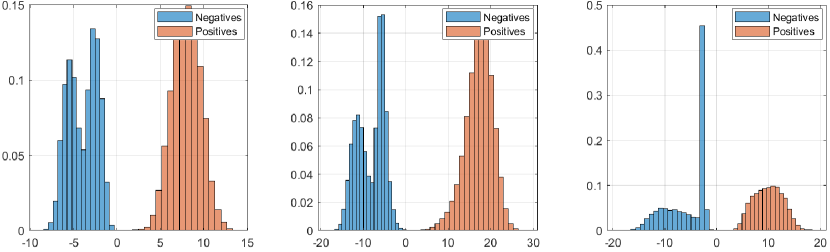
The overconfidence problem is more evident in complex networks such as Convolutional Neural Networks (CNNs), particularly when using the Softmax layer as the prediction layer, thus generating ill-distributed outputs i.e., values close to either zero or one [26] which can be observed in Fig. 1(a) and Fig. 1(b). We note that this is desirable when the true positives have higher scores. However, the counterpart problem is that ‘overconfidence networks’ also generate high-score values for the objects erroneously detected or classified i.e., false positives. Given this problem, a question that arises, how can we guarantee prediction values that are ‘high’ for true positives and, at the same time, ‘low’ for false positives? This question can be answered by analyzing the output of the network’s Logit layer, which provides a smoother output than the Softmax layer. This can be observed within Figs. 2(a) and 2(b).

Following this, we can put a new question: although normalized outputs aim to guarantee a ‘probabilistic interpretation’, how reliable are these predictions? Additionally, given an object belonging to a non-trained/unseen class (e.g., an unexpected object on the road), how confident is the model’s prediction? These are the key research questions explored in this work by considering the importance of having models grounded on interpretable probability assumptions to enable adequate interpretation of the outputs, ultimately leading to more reliable predictions and decisions. In terms of contributions, this paper introduces new prediction layers, designated Maximum Likelihood (ML) and Maximum a-Posteriori (MAP) layers, for deep neural networks, which provide a more adequate solution compared to state-of-the-art (Softmax or Sigmoid) prediction layers. Both ML and MAP layers compute a single estimate, rather than a distribution. Moreover, this work contributes towards the advances of multi-sensor perception (RGB and LiDAR modalities) for autonomous perception systems [35, 36, 37] by proposing a probability-grounded solution that is practical in the sense it can be used in existing (i.e., pre-trained) state-of-the-art models such as Yolo [38].
It is important to emphasize that there is no need to retrain the neural networks when the approach described in this article is employed, because the ML and MAP prediction layers produce outputs based on PDFs obtained from the Logits of already trained networks. Therefore, instead of using the traditional prediction layers (Softmax or Sigmoid) to predict the object scores on a test set, the ML and MAP nonlinearities can be used to make the predictions for the objects scores. Thus, the proposed technique in this paper is practical given that a network has already been trained with Softmax (SM) or Sigmoid (SG) prediction layers. In other words, the ML and MAP layers depend on the Logit’s outputs of the already trained network111A note for the reviewers: this paper is an extension of our workshop-paper [39], as well as an extension of the paper [40]. The main difference between this paper and the two previously mentioned papers is in the analysis of the results through reliability diagrams, considering the expected calibration error, and maximum calibration error metrics. In addition, this paper considers a more detailed analysis regarding the predicted score values on out-of-training distribution test data (unseen class).
In summary, the scientific contributions arising from this work are:
-
•
An investigation of the distribution of predicted values of the Logit and Softmax layers, for both calibrated and non-calibrated networks;
-
•
An analysis of the predicted probabilities inferred by the proposed ML and MAP formulations, both for object classification and detection;
-
•
An investigation of the predicted score values on out-of-training distribution test data (unseen/non-trained class);
-
•
The proposed approach does not require the retraining of networks;
-
•
Experimental validation of the proposed methodology through different modalities, RGB and Range-View (3D point clouds-LiDAR), for classification (using InceptionV3) and object detection (using YoloV4).
In this paper, we report on object recognition results showing that the Softmax and Sigmoid prediction layers do indeed sometimes induce erroneous decision-making, which can be critical in autonomous driving. This is particularly evident when ‘unseen’ samples i.e., out-of-training distribution test data are presented to the network. On the other hand, the approach described here is able to mitigate such problems during the testing stage (prediction).
The rest of this article is structured as follows. The related work is presented in Section II, while the proposed methodology is developed in Section III. The experimental part and the results are reported in Section IV, the conclusion is given in Section V, while Section VI presents ideas to expand the proposed research, and finally Section VII (Appendix) presents results considering an extra experiment.
II Related Work
In this section, we review the key methodologies related to our proposed approach. We briefly discuss the uncertainties of neural networks based on the concepts of Bayesian inference, consequently defining the types of uncertainties that can be captured by the Bayesian Neural Networks (BNNs). Then, techniques for reducing overconfidence of prediction layers are presented as well, in particular the regularization and calibration techniques.
II-A Predictive Uncertainty
Many deep learning methods used for perception systems (objects detection and recognition) do not capture the network uncertainties at training and test times. The Bayesian Neural Network (BNN) is an alternative to cope with uncertainties and it can be carried out through distinct approaches. One way is to obtain the posterior distribution using variational inference after defining a prior distribution to the network weights [32, 41, 42]. Another method is the ensemble of multiple networks with the same architecture and different training sets for estimating predictive uncertainty [43].
Currently, many studies consider aleatory and epistemic uncertainties obtained through BNNs. Aleatory uncertainty is related to the inherent noise of observations (uncertainties arising from sensor inherent noise and associated with the distance of the object to be detected, as well as the object occlusion), while the epistemic ones explain the uncertainties in the model parameters (uncertainties of the model associated with the detection accuracy, showing the limitations of the model) [44]. The formulation of aleatory and epistemic uncertainties with the aim of presenting confidence of predictions, which can capture the uncertainties in object recognition, can be done through BNNs, Shannon Entropy (uncertainty in the prediction output) and Mutual Information (confidence of the model in the output) to measure the uncertainty of the classification scores [45, 46, 47].
The uncertainty of a prediction can also be achieved through Monte Carlo dropout strategy, using the dropout layers at test time i.e., the predicted values depend on the randomly chosen connections between the neurons according to the dropout rate, that is, the same test example (an object) forwarded several times in the network can have different predicted values (the predicted values are not deterministic). In this way, it is possible to obtain the distribution, the average (final predicted value) and the variance (uncertainty) [48] for each example.
Differing from the aforementioned works, the approach proposed in this paper uses data obtained from the Logit layer of already trained/existing networks, to employ the concepts of Bayesian inference. The methodology proposed in this paper defines a final prediction value for each object and does not need to predict recurrently for the same object several times. Furthermore, the approach presented in the paper does not consider the distribution of the network weights, and thus, it is an efficient and practical approach. These advantages are clear when compared to traditional Bayesian neural networks and the Monte Carlo dropout strategy, because the novel strategy presented here avoids a high computational cost and at the same time does preserve the recognition/detection performance. Nevertheless, there are ongoing research on Bayesian neural networks that have reduced the computational cost through feature decomposition and memorization [49].
II-B Regularization and Calibration
Another important component for the improvement of the predicted values are the regularization techniques that avoid overfitting and contribute to reduce overconfidence predictions, such as the transformation of network weights using and [50] regularization, label and model regularization by a process of pseudo-label and self-training [33], label smoothing [51], knowledge distillation [52], architecture development where the network has to determine whether or not an example belongs to the training set, and specific cost mathematical formulation [53, 54]. Other well-known regularization techniques are the Batch Normalization [55], stochastic regularization techniques such as Dropout [56], multiplicative Gaussian noise [57], and dropConnect [58].
Alternatively, highly confident predictions can often be mitigated by calibration techniques such as temperature scaling () [26], by multiplying all the values of the logit vector by a scalar parameter, , for all classes, where the value of is obtained by minimizing the negative log likelihood on the validation set; Isotonic Regression [59] which combines binary probability estimates of multiple classes, thus jointly optimizing the bin boundary and bin predictions; Platt Scaling [60] which uses classifier predictions as features for a logistic regression model; Beta Calibration [61] which uses a parametric formulation that considers the Beta probability density function; compositional method (parametric and non-parametric approaches) [62], as well as the embedding complementary networks technique [63, 64].
In this study, we reduce highly confident predictions on the test set by replacing the predicted values by Softmax and Sigmoid layers with the predicted values from ML and MAP nonlinearities, obtaining a smoother score distribution for new objects. Such functions depend on the output of the network’s Logit layer, by means of parametric (Gaussian functions) and nonparametric (normalized histograms) modeling. This is a post-training operation, that is, the novel inference functions proposed in this work do not modify the weights neither the cost function of the network and still provides very satisfactory results. This is an advantage over regularization techniques, since the ML and MAP layers do not require network retraining. The advantage of the approach proposed in this paper with respect to calibration techniques is to provide a smoother distribution of the predicted values without degrading the results.
III Proposed Method
This section presents the core of the proposed methodology i.e., the formulations for making predictions based on the novel ML and MAP prediction layers. The development of such a methodology begins with the concepts of probabilities, random variables, distribution function, probability density function and Bayes’ theorem i.e., the background to develop the methodology proposed in this paper. In the second stage, we present the proposed method through formulations of the Maximum Likelihood (ML) and Maximum a-Posteriori (MAP) layers, as well as nonparametric and parametric mathematical modeling to define the posterior (likelihood-conditional) and prior probabilities. Finally, we present the network architectures, diagrams for evaluating the calibration of the proposed methodology, and the datasets that have been used in the experiments.
III-A A Brief Review of Probability and Density Functions
The output scores of a supervised classification system with classes, can be formulated according to a random experiment considering a sample space . The numerical outcome obtained from each element of is related to a real number defined by the random variable (rv) x i.e., the output scores, which is conditioned to the rv . Formally, the rv is a function that maps each element of the sample space with a real number of the set , which can be simply expressed as . In other words, an rv is a function x that outputs a real number for each element of a random experiment. From the sample space, an event (subset of ) can be defined and associated with a probability between the , interval. Such probability is a distribution function and its derivative is the probability density function (PDF) , as in (1) [65].
| (1) |
where , considering continuous. The integral of (1) represents the probability with the random variable x contained in the interval. Consequently, if the interval [, ] is sufficiently small, the probability will be i.e., the probability of the random variable x is proportional to . Thus, the probability will be maximum if the interval [, ] contains its value and will be maximum. Such a value is the most likely value of x.
Given the most likely value of the random variable x, Maximum Likelihood (ML) and Maximum a-Posteriori (MAP) inferences can be obtained. However, the random variable x is dependent of the variable c for the formulation of ML and MAP. Therefore, the density function is conditional to c [65], as formulated in (2):
| (2) |
If the random variable is discrete, a probability mass function (PMF) is used instead of a probability density function (PDF). Assuming that the class conditional probability (likelihood) and the prior are known, the posterior probability can be obtained through Bayes’ rule
| (3) |
where is the prior probability, is the marginal probability defined by , that often can be determined by law of the total probability [66]. Thus, (3) can be re-written using the per-class expression:
| (4) |
In this work, the goal is to use (4) to make inferences on the test set about the ‘unknown’ rv c from the dependence with x i.e., the value of the posterior distribution of c is determined after observing the value of x.
III-B ML and MAP Prediction Layers


The proposed ML and MAP layers make inference based on PDFs obtained from the Logit layer prediction scores by using the training set. This is illustrated in Fig. 3, where the horizontal axes represent the random variable x and the vertical axes are the normalized frequency of the amount of objects in the classification and detection datasets. We can observed that the distribution scores from the Logit layer are far more appropriate to represent a PDF (as shown in Fig. 2). Therefore, the ML and MAP layers are more adequate to perform probabilistic inference in regard to permitting decision-making under uncertainty, which is particularly relevant in autonomous driving and robotic perception systems.
As noted in (4), the posterior probability depends on the class conditional probability (likelihood function) and on the prior probability i.e., the MAP estimated depends on a distribution for both the likelihood and prior, while ML only depends on , because is usually assumed to be uniform and identically distributed. The probabilities are modeled by means of non-parametric estimates over the predicted scores of the Logit layer for each class, as showed in the first column of Fig. 3. These estimates are obtained on the training set, through normalized histograms (i.e., discrete densities defined by a single parameter - the number of bins) for each modality, as shown in the Table I.
Histograms are graphical ways of summarizing or describing a variable in a simple way, in other words, histograms show how variables (in this case, the network logits) are distributed, revealing modes and bumps, as well as information about the frequencies of observations. As said by C. Bishop [66], ‘we can view the histogram as a simple way to model a probability distribution given only a finite number of points drawn from that distribution’. Often, the bins of a histogram are chosen to have the same width thus, the only (single) parameter left is the number of bins (nbins). To do so, nbins can be mathematically determined by means of the mean squared error (MSE-expected value of the squared error) [67]. However, for our methodology, we have chosen nbins empirically to guarantee a result very close to or better than the results provided by the SM and SG layers and, in addition, to generate smoother distribution by adding the parameter . Thus, the process of estimating the number of bins and (the additive smoothing factor) have been defined empirically by verifying which combinations would not degrade the results. So, these two parameters were defined empirically for each dataset/modality, as well as for each of the ML and MAP layers.
| Maximum Likelihood | ||||||||
| RGB Modalitiy | RV Modality | |||||||
| Dataset | Bins |
|
Bins |
|
||||
| KITTI | ||||||||
| LL5 | ||||||||
| Maximum a-Posteriori | ||||||||
| RGB Modalitiy | RV Modality | |||||||
| Dataset | Bins |
|
Bins |
|
||||
| KITTI | ||||||||
| LL5 | ||||||||
Each predicted value on the test set from the Logit layer has a score value corresponding to its bin range in the respective class histogram, which is illustrated in Fig. 4. For the MAP layer, the prior is modeled by a Gaussian distribution that guarantees a smoother distribution of the prediction values, as observed within the second column of Fig. 3. Thus, with mean and variance is calculated per class, from the training set. The modeling with different distribution techniques, Gaussian distribution and normalized histogram, aims to capture complementary information from the training data, where the maximum values per classes in the normalized histograms are different from the maximum values of the Gaussian distributions (Fig. 3).
The normal distribution is feasible for modeling an unknown distribution because it has a maximum entropy. Thus, the greater entropy can guarantee a more informative distribution and at the same time less confident information around the mean, that is, it contributes to the reduction of the overconfidence inferences. Defining otherwise, the events most likely to happen have low information content i.e., low entropy. Therefore, a Gaussian distribution was defined for prior to express a high degree of uncertainty222The amount of uncertainty can be quantified, for example, using Shannon’s entropy for a probability distribution. in the value of variable c before observing the data. Furthermore, a prior distribution with high entropy is said to be a prior distribution with high variance [66].

Additionally, to avoid the ‘zero’ probability problem, as well as to incorporate some uncertainty level in the final prediction, the Additive Smoothing method () [68, 69, 70] (also defined as Laplace smoothing) is implemented during the ML and MAP predictions. The values assigned for the Additive Smoothing are shown in Table I, does not depend on previous information of the training set. This value was determined empirically i.e., by observing which value would preserve approximately the ‘original’ distribution without compromising the final result. The probability estimates with the Additive Smoothing are shown in (5) and (6), i.e., a small correction is incorporated into the ML and MAP estimate. Consequently, no prediction will have a ‘zero’ probability, no matter how unlikely.
ML layer is straightforwardly calculated by normalizing by the during the prediction phase, as in (5), since the priors are set uniformly and identically distributed for the set of classes c,
| (5) |
Alternatively, the inference using MAP layer is given in (6) as follows,
| (6) |
The sequential steps for calculating the ML and MAP is summarized within Algorithm 1, where class-conditional is modelled by a normalized histogram. On the other hand, to get the maximum posterior probabilities (MAP) the priors are modelled by normals , where the sub-index indicates that the data is obtained from the Logit layer (layer before the network prediction layer). Both the likelihood and prior are extracted from the Logit layer using the training data333The code for training the network, obtaining the logit layers and computing the ML and MAP layers are available at github.com/gledsonmelotti/ML-MAP-Layers-for-Probabilistic..
III-C CNN Architectures for Object Recognition

Experiments in [26] suggested that the greater the number of layers and neurons, the more overconfidence the result will be. However, the experiments that we have conducted show that even when reducing the amount of neurons and filters in the dense and convolutional layers, the network can still produce overconfidence in the predicted values, as can be observed in Fig. 1. This conclusion was reached by training the Inception V3 CNN [71] and reducing the number of filters and neurons/units. Regarding object detection, the model Yolo V4 [38] was trained to detect cars, cyclists, and pedestrians, with predictions based on the SG layer.
The experiments reported throughout the remainder of this work were based on the premise that, after training the network, the proposed ML and MAP layers then replace the SM and SG prediction layers on the test set, only, according to Fig. 5.
III-D Reliability Diagram

Typically, post-calibration predictions are analyzed in the form of reliability diagram representations [72, 26], which illustrate the relationship of the model’s prediction scores in regard to the true correctness likelihood [73], as shown in Fig. 6. Reliability diagrams show the expected accuracy of the samples as a function of confidence i.e., the maximum value of the prediction function.
The scores (predicted values) are grouped into bins (histogram) in the reliability diagrams. Each sample (classification score of an object) is allocated within a bin, according to the maximum prediction value (prediction confidence). Each bin has a range , where . The accuracy is calculated in each range , as well as the average confidence , where is the confidence for sample and is the amount of objects in each . In addition, a gap can be obtained i.e., the difference between accuracy and average confidence in each range (). Thus, the greater the gap, the worse the calibration result in the respective bin. Furthermore, through reliability diagrams, it is possible to obtain calibration errors, such as the Expected Calibration Error (ECE) and the Maximum Calibration Error (MCE):
| (7) | |||
| (8) |
where n is the number of samples.
III-E Benchmarking Datasets
| KITTI dataset - 7481 Frames | |||
|---|---|---|---|
| Car | Cyclist | Pedestrian | |
| Training | |||
| Validation | |||
| Testing | |||
| Non-trained (‘unseen-adversarial’) objects | |||
| Tram/Truck/Van | Tree/lamppost | Person-sitting | |
| Training | - | - | - |
| Validation | - | - | - |
| Testing | |||
| LL5 dataset - 158757 Frames | |||
| Car | Cyclist | Pedestrian | |
| Training | |||
| Validation | |||
| Testing | |||
| Non-trained (‘unseen-adversarial’) objects | |||
| Bus/OtherVehicle/Truck | Tree/lamppost | Motorcycle | |
| Training | - | - | - |
| Validation | - | - | - |
| Testing | |||


A key contribution to the growing improvement of perception systems for autonomous driving is the availability of representative datasets of different modalities, such as RGB, LiDAR, and radar [74, 75, 76, 77, 78, 79]. In this work, we used the KITTI Vision Benchmark Suite- object [36] and Lyft Level-5 (LL5) Perception [80, 81] datasets. The classes of interest were pedestrians, cars, and cyclists. Table II shows the number of objects cropped from both the RGB and range-view (depth from the LiDAR modality) images. In addition, some extra objects from the unseen/non-trained classes (not used during training), such as a person sitting, tram, truck, van, tree, lamppost, signpost, bus, and motorcycle classes were classified in the test/prediction phase, to verify the erroneous overconfidence from the prediction layers of the trained networks. Such a class can be understood as an ‘adversarial’ class; Note that this research did not carry out any study involving adversarial network architectures.
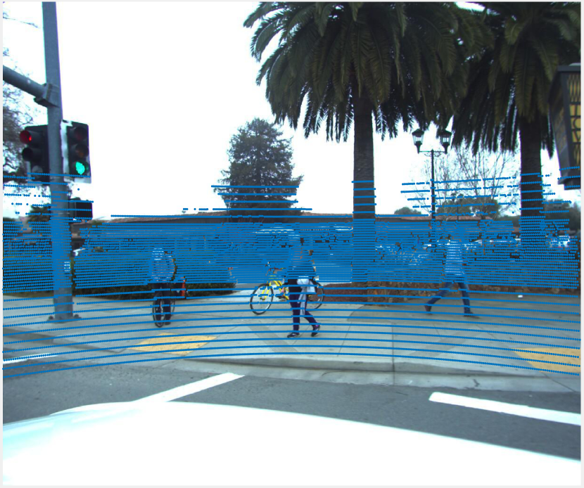
Range-view images were obtained by a coordinate transformation of the point clouds on the image plane followed by an upsample of the projected points. The upsample was performed using a bilateral filter, and considered a mask size (sliding-windows) [37, 82, 83, 84] for t he KITTI dataset and a mask size for LL5 dataset. Examples of these operations can be observed in Fig. 7 and Fig. 8, respectively.
As a way to validate the proposed methodology for object detection, the KITTI Vision Benchmark Suite- object was used. The respective dataset was divided into frames for the training dataset, frames for the validation dataset and frames for the test dataset.
IV Evaluation and Results
The output scores of the CNN indicate a degree of certainty of the given prediction. The level of certainty can be defined as the confidence of the model, and in an object recognition problem, represents the maximum value within the prediction layer. However, the output scores may not always represent a reliable indication of certainty with regard to a given class, especially when unseen (non-trained) objects occur in the prediction stage; this is particularly relevant for a real world application involving autonomous robots and vehicles, since unpredictable objects are likely to be encountered which would be misclassified by prediction layers with a high degree of certainty. With this in mind, in addition to the trained classes (pedestrian, car, and cyclist), a set of unseen objects were introduced into the classification dataset, according to Subsection III-E. Regarding the object detection, the unseen classes are already contained in the dataset’s own frames. Unlike the results reported on the classification dataset, the object detection results are presented by means of precision-recall curves considering the easy, moderate, and hard cases, according to the devkit-tool provided by the KITTI benchmark.
IV-A Results on Object Classification
| KITTI dataset | ||||||
|---|---|---|---|---|---|---|
| Modalities | ||||||
| F-score | ||||||
| LL5 dataset | ||||||
| Modalities | ||||||
| F-score | ||||||
All classes for the training dataset were extracted directly from the aforementioned datasets, except for the tree, lamppost, and signpost classes which were manually extracted from the data for this study. The rationale behind this is to evaluate the prediction confidence of the network on objects that do not belong to any of the trained classes, and as such the consistency of the models can be assessed. Ideally, if the classifiers are perfectly consistent in terms of probability interpretation, the prediction scores would be identical (equal to ) for each class in each sample of the unseen dataset. Results on the testing set are shown in Table III in terms of F-score, false positive rate (), the average () and variance () of the false positives (). The average () and the variance () of the predicted scores are also shown for the unseen testing set (out-of-training distribution test data).
In reference to Table III, where the results are reported based on the classification test set, it can be observed that the , and values are considerably lower than the results presented by the SM layer for both of the sensor modalities and datasets. Regarding the F-scores of the proposed approach (ML and MAP) compared to the SM resulted in an average reduction of (percentage point) for the RGB modality and for RV modality, considering KITTI dataset. The F-scores on the LL5 dataset got a gain of for RGB modality, considering the MAP approach, F-score of the VR modality had a average reduction of . Such reductions of the F-scores are relatively small and thus did not compromise the classification ability. Additionally, the distribution of the top-label scores on the test set comprising the objects that belong to the trained classes (in-distribution classes) is discussed in the Appendix VII-A.
Another way of analyzing the results of reducing overconfidence predictions is through reliability diagrams, as shown in the figures 9 and 10, considering uncalibrated, ML and MAP data. Furthermore, as a way of validating our methodology, we compared our results achieved with the temperature scaling calibration technique. Note that the results presented through the reliability diagrams are shown through the MCE and ECE metrics. From these metrics we cannot say which is the best calibration technique, because for a given technique the lowest value for the MCE was obtained, while for another technique the lowest value for the ECE was obtained. However, we show that the proposed approach contributed to reduce the calibration errors i.e., to reduce the values of the MCE and ECE metrics when compared to the uncalibrated data, and consequently we provide a more reliable result, as well as the contribution to reduce the overconfidence predictions.


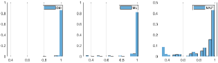
Further experiments have been carried out as a complementary analysis concerning the network’s overconfidence behaviour, on a so-called ‘unseen’ test set, by means of the network’s average score . Note that for ML and MAP layers, the results are smaller than the SM layer as can be seen in Table III. This indicates that the probabilistic inferences are significantly better balanced i.e., enabling more reliable decision-making, when ‘new’ objects of ‘non-trained’ classes are presented to the CNNs, as illustrated by Fig. 11 i.e., the distribution for the unseen dataset. We can see that the aforementioned graphs show less extreme results than those provided by the SM layer.


IV-B Results on Object Detection
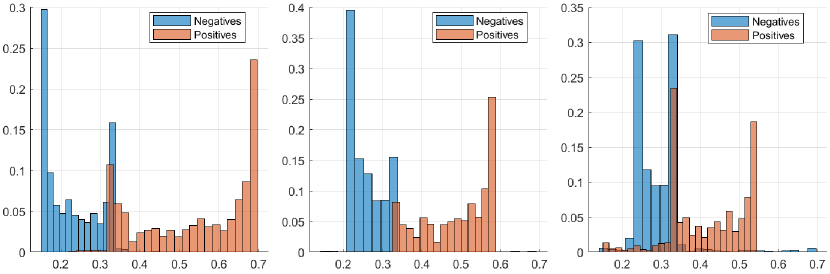
The results on the object detection dataset using the ML and MAP nonlinearities are impressive. Such results were not presented through reliability diagrams, but through normalized histograms, which showed more clearly the reduction in overconfidence in relation to objects detected as false positives without degrading the results of the true positives, as showed in Fig. 12. The results are more representative through precision-recall curves, especially for the cyclist class (Cyc), whose areas under the curves (AUCs) are , and for the easy, moderate and hard cases respectively, as shown in Fig. 13 and Table IV. With respect to the car (Car) and pedestrians (Ped), the proposed approach also showed some improvement.
| Easy | Moderate | Hard | |||||||||
|---|---|---|---|---|---|---|---|---|---|---|---|
| SG | ML | MAP | SG | ML | MAP | SG | ML | MAP | |||
| Car | Car | Car | |||||||||
| Cyc | Cyc | Cyc | |||||||||
| Ped | Ped | Ped | |||||||||

Note that the proposed methodology is dependent on the number of bins () and the parameter . Thus, the values of the scores may vary according to the values of these parameters. For the particular case of the cyclist class, the proposed methodology achieved strong classification performance compared to the baseline (results in Table IV). In this paper we have chosen to use a single set of parameters for all the three cases (i.e., the same values of and for each class). Given the proposed approach, we note that a set of tailored parameters for each class can be used instead, as the distributions (PDF’s) are carried out individually.
V Discussion and Conclusion
Within the experiments performed in this work, a probabilistic approach for CNNs was addressed as distributions in the Logit layer to better represent the classification outputs. The results reported within the experiments in this work are promising given that ML and MAP noticeably reduced the classifier overconfidence and provided a more significant distribution in terms of probabilistic interpretation.
The improvement is not as significant when analyzing objects defined as true positives. But, our concern is to develop a methodology that can reduce the values of false positives (mainly objects of the unseen class: which may be critical in robotics and autonomous driving applications) without degrading the results achieved by true positives. Note that we have included two metrics in Table III, in order to show the reduction of score values for the ‘unseen’ class (in particular) and also to show that the overconfidence behavior has been mitigated for TPs and FPs.
One potential way to improve the F-scores achieved by the ML and MAP layers would be to obtain a ‘perfect’ match between the smoothing parameter () and the number of bins in the histograms. For the new results with the EfficientNetB1 network, we have selected the parameters by using an exhaustive search process (combining several values as possible), in order to keep the values of the F-scores of the ML and MAP layers practically identical to those achieved by the EfficientNetB1 baseline. Figures 16, 17, and 18 show reductions on the scores for objects of class ‘unseen’ thus, the proposed approach is efficient.
As a consequence of the Additive Smoothing, the score values equal to and are excluded from the prediction values. The influence of the parameter on the data distribution can be seen from the figures in Appendix VII-B, particularly with respect to objects of the ‘unseen’ class.
To assess the classifier’s robustness or the uncertainty of the model when predicting objects of unseen classes by the network, we considered a test set comprised of ‘new’ objects. Overall, the results are promising, since the distribution of the predictions were not extremities relative to the results from the SM layer, in other words, the average scores using ML and MAP layers were significantly lower than the Softmax prediction layer (the baseline), and thus the CNNs are less prone to overconfidence.
The results for object classification were presented through reliability diagrams, taking into account the MCE and ECE metrics. In fact, such metrics indicate how much the predicted score values are calibrated, that is, the best calibration has to present the lowest value for the MCE and ECE. However, we observed that depending on the dataset and sensor modality, our approach obtained the best result in only one of the metrics i.e., either the lowest value for the MCE metric or the lowest value for the ECE metric. This fact can also be noticed with the temperature scaling calibration technique.
Another important factor that contributes to validate the proposed approach is the use of two different datasets, in terms of both RGB and Range-View ( point clouds-LiDARs) modalities, since the sensors of the datasets have different resolutions, mainly the LiDAR sensor; While the KITTI dataset provides point clouds obtained from a sensor with 64 beams, the LL5 dataset provides point clouds with 40 beams - and so, the proposed approach was also successful with differing sensor resolutions within the state of the art.
The proposed methodology also obtained good results for object detection, not degrading the results when compared to the SG prediction layer, presenting better results in all cases. The improvement is more evident for the ‘cyclist’ class, which contains the least amount of examples. This is an interesting result that could be further investigated in future work.
Regarding the formulations of probabilistic distributions, the prior modeling by a Gaussian distribution was shown to guarantee a smoother distribution for the prediction values. Unlike the prior, the likelihood function was modeled by means of a normalized histogram i.e., by a non-parametric formulation showing the probability distributions. If both the prior and the likelihood function were modeled by a uniform distribution, the final result would be similar to those achieved by the SM and SG layers, since it would not offer any smoothing for the prediction values. In fact, a uniform prior or likelihood would add a constant to the training data modeling, which would have little effect on the prediction values obtained by the ML and MAP .
VI Future Work
Softmax and Sigmoid layers represent confidence measures, but they do not provide any measure of uncertainty of the predictions. In other words, both layers mentioned previously provide a direct measure of certainty through the maximum class probability. Such layers also do not provide any information about the certainty that the model itself has about the predictions. Therefore, we address the issues of overconfident predictions and calibration techniques in this work with a focus on perception systems for autonomous vehicles. However, we realize that there is a lack of studies on how to quantify the certainty/uncertainty of predictions in relation to calibration techniques and reliability diagrams. As we verified that the MCE and ECE metrics that quantify the calibrated data through the reliability diagrams depend on the number of bins of such diagrams, that is, by changing the number of bins, the MCE and ECE metrics can provide new error values. Thus, what is the correct value of bins to ensure that a set of predictions is well calibrated?
Regardless of the methodology to reduce overconfidence predictions or capture uncertainty in predictions, how should we assess the quality of estimated uncertainty independent of calibration and regularization techniques?
Faced with such questions and based on the studies presented in the literature on computing uncertainties of predictions and of calibration and regularization techniques, we found that evaluating the quality of uncertainty estimates is still a challenge for the following reasons:
-
•
uncertainty estimates depend on methods, which are performed by means of approximations i.e., by means of inferences;
-
•
uncertainty estimates depend on the sample size i.e., the sample size can provide a certain degree of confidence that such a sample is representative;
-
•
it is not easy to obtain a ground truth about uncertainty estimates. In fact, during our study we did not verify the ground truth about uncertainty estimates;
-
•
study and evaluate the quality of quantitative uncertainty metrics, such as entropy, Mutual Information, Kullback-Leibler Divergence, and predictive variance.
Based on the issues mentioned above, we intend to advance research on the quality of uncertainty estimates, including the formulation of reliability diagrams, as a way to quantify the quality of uncertainty estimates.
VII Appendix
VII-A Prediction Scores of the Objects on the Testing Set
The proposed methodology, which is based on the ML/MAP layers, aims to reduce overconfidence predictions of deep models, especially for objects classified as false positives which sometimes receive high score values of deep networks. An ideal result would be for the network to provide lower score values for the false positives i.e., objects misclassified by the network, and concurrently to attain higher scores for the true positives. As a way of validating additional results on test sets, we present the Fig. 14 and Fig. 15 that contain the results for the pedestrian, car, and cyclist classes (columns from left to right), considering the scores of the objects as being positive and negative, which show smoother distributions of scores when compared to the results shown in Fig. 1.


VII-B Smoothing Parameter Influence
Additionally to the results presented above, we have implemented the proposed methodology on another state-of-the-art network, the EfficientNetB1. The performance achieved by the EfficientNetB1 to classify RGB images is a F-score of using the Softmax layer (as baseline). The result achieved through the ML layer is equivalent to the baseline i.e., F-score = , while using the MAP layer the network achieved (almost the same). By keeping for both cases, we have performed several runs by changing the values of , and the resulting F-score stabilized around i.e., very close to the F-score provided by the Softmax layer (baseline). A way to choose the best values for nbins and could be, for instance, by reducing the values of the scores of the objects classified as false positives without degrading the results of the true positives, as illustrated by figures 16, 17, and 18, where the distributions in each row were obtained through a given value for the parameter, considering classifications from the unseen dataset. Note that as the value of increases, the distributions tend to move away from the extreme values ( and ).


References
- [1] C. Patel, D. Bhatt, U. Sharma, R. Patel, S. Pandya, K. Modi, N. Cholli, A. Patel, U. Bhatt, M. A. Khan, S. Majumdar, M. Zuhair, K. Patel, S. A. Shah, and H. Ghayvat, “Dbgc: Dimension-based generic convolution block for object recognition,” Sensors, vol. 22, no. 5, 2022.
- [2] D. Bhatt, C. Patel, H. Talsania, J. Patel, R. Vaghela, S. Pandya, K. Modi, and H. Ghayvat, “Cnn variants for computer vision: History, architecture, application, challenges and future scope,” Electronics, vol. 10, no. 20, 2021.
- [3] J. Janai, F. Güney, A. Behl, and A. Geiger, “Computer vision for autonomous vehicles: Problems, datasets and state of the art,” Foundations and Trends in Computer Graphics and Vision, vol. 12, no. 1–3, pp. 1–308, 2020.
- [4] S. Liu, L. Li, J. Tang, S. Wu, and J.-L. Gaudiot, “Creating autonomous vehicle systems,” Synthesis Lectures on Computer Science, vol. 6, no. 1, pp. i–186, 2017.
- [5] C. I. Patel, S. Garg, T. Zaveri, and A. Banerjee, “Top-down and bottom-up cues based moving object detection for varied background video sequences,” Advances in Multimedia, Hindawi Publishing Corporation, vol. 2014, 2014.
- [6] T. Hehn, J. F. P. Kooij, and D. M. Gavrila, “Fast and compact image segmentation using instance stixels,” IEEE Transactions on Intelligent Vehicles, pp. 1–1, 2021.
- [7] Z. Wang, D. Feng, Y. Zhou, L. Rosenbaum, F. Timm, K. Dietmayer, M. Tomizuka, and W. Zhan, “Inferring spatial uncertainty in object detection,” in EEE/RSJ International Conference on Intelligent Robots and Systems, 2020, pp. 5792–5799.
- [8] P. Cai, Y. Sun, H. Wang, and M. Liu, “VTGNet: A vision-based trajectory generation network for autonomous vehicles in urban environments,” IEEE Transactions on Intelligent Vehicles, pp. 1–1, 2020.
- [9] M. Schutera, M. Hussein, J. Abhau, R. Mikut, and M. Reischl, “Night-to-day: Online image-to-image translation for object detection within autonomous driving by night,” IEEE Transactions on Intelligent Vehicles, pp. 1–1, 2020.
- [10] H. Pan, Z. Wang, W. Zhan, and M. Tomizuka, “Towards better performance and more explainable uncertainty for 3d object detection of autonomous vehicles,” in IEEE 23rd International Conference on Intelligent Transportation Systems, 2020, pp. 1–7.
- [11] X. Cai, M. Giallorenzo, and K. Sarabandi, “Machine learning-based target classification for MMW radar in autonomous driving,” IEEE Transactions on Intelligent Vehicles, pp. 1–1, 2021.
- [12] C. Zhou, Y. Liu, P. Lasang, and Q. Sun, “Vehicle detection and disparity estimation using blended stereo images,” IEEE Transactions on Intelligent Vehicles, pp. 1–1, 2021.
- [13] J. Nie, J. Yan, H. Yin, L. Ren, and Q. Meng, “A multimodality fusion deep neural network and safety test strategy for intelligent vehicles,” IEEE Transactions on Intelligent Vehicles, pp. 1–1, 2020.
- [14] D. Feng, C. Haase-Schütz, L. Rosenbaum, H. Hertlein, C. Gläser, F. Timm, W. Wiesbeck, and K. Dietmayer, “Deep multi-modal object detection and semantic segmentation for autonomous driving: Datasets, methods, and challenges,” IEEE Transactions on Intelligent Transportation Systems, vol. 22, no. 3, pp. 1341–1360, 2021.
- [15] C. Li, W. Xia, Y. Yan, B. Luo, and J. Tang, “Segmenting objects in day and night: Edge-conditioned cnn for thermal image semantic segmentation,” IEEE Transactions on Neural Networks and Learning Systems, pp. 1–14, 2020.
- [16] Z. Zuo, X. Yang, Z. Li, Y. Wang, Q. Han, L. Wang, and X. Luo, “Mpc-based cooperative control strategy of path planning and trajectory tracking for intelligent vehicles,” IEEE Transactions on Intelligent Vehicles, pp. 1–1, 2020.
- [17] M. M. D. Santos, J. E. Hoffmann, H. G. Tosso, A. W. Malik, A. U. Rahman, and J. F. Justo, “Real-time adaptive object localization and tracking for autonomous vehicles,” IEEE Transactions on Intelligent Vehicles, pp. 1–1, 2020.
- [18] D. Su, H. Zhang, H. Chen, J. Yi, P.-Y. Chen, and Y. Gao, “Is robustness the cost of accuracy? A comprehensive study on the robustness of 18 deep image classification models,” in European Conference on Computer Vision, 2018.
- [19] M. Sensoy, L. Kaplan, and M. Kandemir, “Evidential deep learning to quantify classification uncertainty,” in Advances in Neural Information Processing Systems 31, 2018, pp. 3179–3189.
- [20] Š. Raudys, R. Somorjai, and R. Baumgartner, “Reducing the overconfidence of base classifiers when combining their decisions,” in Multiple Classifier Systems, 2003, pp. 65–73.
- [21] K. B. Bulatov and D. V. Polevoy, “Reducing overconfidence in neural networks by dynamic variation of recognizer relevance,” in Proceedings 29th European Conference on Modelling and Simulation, 2015, pp. 488–491.
- [22] A. Kristiadi, M. Hein, and P. Hennig, “Being bayesian, even just a bit, fixes overconfidence in ReLU networks,” in Proceedings of the 37th International Conference on Machine Learning, vol. 119, 2020, pp. 5436–5446.
- [23] S. Thulasidasan, G. Chennupati, J. A. Bilmes, T. Bhattacharya, and S. Michalak, “On mixup training: Improved calibration and predictive uncertainty for deep neural networks,” in Advances in Neural Information Processing Systems 32, 2019, pp. 13 888–13 899.
- [24] C. Gupta, A. Podkopaev, and A. Ramdas, “Distribution-free binary classification: prediction sets, confidence intervals and calibration,” in Advances in Neural Information Processing Systems, 2020, pp. 3711–3723.
- [25] C. Gupta and A. K. Ramdas, “Top-label calibration and multiclass-to-binary reductions,” in Proceedings of the International Conference on Learning Representations, 2022.
- [26] C. Guo, G. Pleiss, Y. Sun, and K. Q. Weinberger, “On calibration of modern neural networks,” in Proceedings of the 34th International Conference on Machine Learning, vol. 70, 2017, pp. 1321–1330.
- [27] M. Abdar, F. Pourpanah, S. Hussain, D. Rezazadegan, L. Liu, M. Ghavamzadeh, P. Fieguth, X. Cao, A. Khosravi, U. R. Acharya, V. Makarenkov, and S. Nahavandi, “A review of uncertainty quantification in deep learning: Techniques, applications and challenges,” Information Fusion, vol. 76, pp. 243–297, 2021.
- [28] J. Mena, O. Pujol, and J. Vitrià, “A survey on uncertainty estimation in deep learning classification systems from a bayesian perspective,” ACM Comput. Surv., vol. 54, no. 9, 2021.
- [29] B. Zadrozny and C. Elkan, “Obtaining calibrated probability estimates from decision trees and naive bayesian classifiers,” in Proceedings of the Eighteenth International Conference on Machine Learning. Morgan Kaufmann Publishers Inc., 2001, p. 609–616.
- [30] M. P. Naeini, G. F. Cooper, and M. Hauskrecht, “Binary classifier calibration: Non-parametric approach,” arXiv preprint arXiv:1401.3390, 2014.
- [31] G. Pereyra, G. Tucker, J. Chorowski, L. Kaiser, and G. E. Hinton, “Regularizing neural networks by penalizing confident output distributions,” CoRR, arXiv, vol. abs/1701.06548, 2017.
- [32] K. Posch and J. Pilz, “Correlated parameters to accurately measure uncertainty in deep neural networks,” IEEE Transactions on Neural Networks and Learning Systems, vol. 32, no. 3, pp. 1037–1051, 2021.
- [33] Y. Zou, Z. Yu, X. Liu, B. V. K. V. Kumar, and J. Wang, “Confidence regularized self-training,” in IEEE International Conference on Computer Vision, 2019, pp. 5981–5990.
- [34] J. Gawlikowski, C. R. N. Tassi, M. Ali, J. Lee, M. Humt, J. Feng, A. M. Kruspe, R. Triebel, P. Jung, R. Roscher, M. Shahzad, W. Yang, R. Bamler, and X. X. Zhu, “A survey of uncertainty in deep neural networks,” CoRR, arXiv, vol. abs/2107.03342, 2021.
- [35] M. Martin, A. Roitberg, M. Haurilet, M. Horne, S. Reiss, M. Voit, and R. Stiefelhagen, “Driveact: A multi-modal dataset for fine-grained driver behavior recognition in autonomous vehicles,” in International Conference on Computational Vision, 2019.
- [36] A. Geiger, P. Lenz, and R. Urtasun, “Are we ready for autonomous driving? the KITTI vision benchmark suite,” in IEEE Conference on Computer Vision and Pattern Recognition, 2012, pp. 3354–3361.
- [37] G. Melotti, C. Premebida, and N. Gonçalves, “Multimodal deep-learning for object recognition combining camera and LIDAR data,” in IEEE International Conference on Autonomous Robot Systems and Competitions, 2020, pp. 177–182.
- [38] A. Bochkovskiy, C.-Y. Wang, and H.-Y. M. Liao, “Yolov4: Optimal speed and accuracy of object detection,” CoRR, arXiv, vol. abs/2004.10934, 2020.
- [39] G. Melotti, C. Premebida, J. J. Bird, D. R. Faria, and N. Gonçalves, “Probabilistic object classification using CNN ML-MAP layers,” in Workshop on Perception for Autonomous Driving, European Conference on Computer Vision, 2020.
- [40] G. Melotti, W. Lu, D. Zhao, A. Asvadi, N. Gonçalves, and C. Premebida, “Probabilistic approach for road-users detection,” CoRR arxiv, vol. abs/2112.01360, 2021.
- [41] K. Shridhar, F. Laumann, and M. Liwicki, “A comprehensive guide to bayesian convolutional neural network with variational inference,” CoRR, arXiv, vol. abs/1901.02731, 2019.
- [42] A. Graves, “Practical variational inference for neural networks,” in Advances in Neural Information Processing Systems 24, 2011, pp. 2348–2356.
- [43] B. Lakshminarayanan, A. Pritzel, and C. Blundell, “Simple and scalable predictive uncertainty estimation using deep ensembles,” in Advances in Neural Information Processing Systems 30, 2017, pp. 6402–6413.
- [44] A. Kendall and Y. Gal, “What uncertainties do we need in bayesian deep learning for computer vision?” in Advances in Neural Information Processing Systems 30, 2017, pp. 5574–5584.
- [45] R. McAllister, Y. Gal, A. Kendall, M. van der Wilk, A. Shah, R. Cipolla, and A. Weller, “Concrete problems for autonomous vehicle safety: Advantages of bayesian deep learning,” in Proceedings of the Twenty-Sixth International Joint Conference on Artificial Intelligence, 2017, pp. 4745–4753.
- [46] D. Feng, L. Rosenbaum, F. Timm, and K. Dietmayer, “Leveraging heteroscedastic aleatoric uncertainties for robust real-time lidar 3D object detection,” in IEEE Intelligent Vehicles Symposium, 2019, pp. 1280–1287.
- [47] D. Feng, L. Rosenbaum, and K. Dietmayer, “Towards safe autonomous driving: Capture uncertainty in the deep neural network for lidar 3D vehicle detection,” in IEEE 21st International Conference on Intelligent Transportation Systems, 2018, pp. 3266–3273.
- [48] Y. Gal and Z. Ghahramani, “Dropout as a bayesian approximation: Representing model uncertainty in deep learning,” in Proceedings of The 33rd International Conference on Machine Learning, vol. 48, 2016, pp. 1050–1059.
- [49] X. Jia, J. Yang, R. Liu, X. Wang, S. D. Cotofana, and W. Zhao, “Efficient computation reduction in bayesian neural networks through feature decomposition and memorization,” IEEE Transactions on Neural Networks and Learning Systems, pp. 1–10, 2020.
- [50] A. Y. Ng, “Feature selection, L1 vs. L2 regularization, and rotational invariance,” in Proceedings of the twenty-first international conference on Machine learning, 2004.
- [51] M. Lukasik, S. Bhojanapalli, A. Menon, and S. Kumar, “Does label smoothing mitigate label noise?” in PMLR Proceedings of the 37th International Conference on Machine Learning, vol. 119, 2020, pp. 6448–6458.
- [52] G. Hinton, O. Vinyals, and J. Dean, “Distilling the knowledge in a neural network,” in NIPS Deep Learning and Representation Learning Workshop, 2015.
- [53] C. Corbière, N. THOME, A. Bar-Hen, M. Cord, and P. Pérez, “Addressing failure prediction by learning model confidence,” in Advances in Neural Information Processing Systems, vol. 32, 2019.
- [54] T. DeVries and G. W. Taylor, “Learning confidence for out-of-distribution detection in neural networks,” CoRR, arXiv, vol. abs/1802.04865, 2018.
- [55] S. Ioffe and C. Szegedy, “Batch normalization: Accelerating deep network training by reducing internal covariate shift,” in Proceedings of the 32nd International Conference on Machine Learning, vol. 37, 2015, pp. 448–456.
- [56] G. E. Hinton, N. Srivastava, A. Krizhevsky, I. Sutskever, and R. Salakhutdinov, “Improving neural networks by preventing co-adaptation of feature detectors,” CoRR, arXiv, vol. abs/1207.0580, 2012.
- [57] N. Srivastava, G. Hinton, A. Krizhevsky, I. Sutskever, and R. Salakhutdinov, “Dropout: A simple way to prevent neural networks from overfitting,” Journal of Machine Learning Research, vol. 15, pp. 1929–1958, 06 2014.
- [58] L. Wan, M. Zeiler, S. Zhang, Y. L. Cun, and R. Fergus, “Regularization of neural networks using dropconnect,” in Proceedings of the 30th International Conference on Machine Learning, vol. 28, no. 3, 2013, pp. 1058–1066.
- [59] B. Zadrozny and C. Elkan, “Transforming classifier scores into accurate multiclass probability estimates,” in Proceedings of the Eighth ACM SIGKDD International Conference on Knowledge Discovery and Data Mining, 2002, pp. 694––699.
- [60] J. C. Platt, “Probabilistic outputs for support vector machines and comparisons to regularized likelihood methods,” in Advances Large Margin Classifiers, 2000, pp. 61–74.
- [61] M. Kull, T. Silva Filho, and P. Flach, “Beta calibration: a well-founded and easily implemented improvement on logistic calibration for binary classifiers,” in 20th AISTATS., 2017, pp. 623–631.
- [62] J. Zhang, B. Kailkhura, and T. Han, “Mix-n-match: Ensemble and compositional methods for uncertainty calibration in deep learning,” in International Conference on Machine Learning (ICML), 2020.
- [63] Q. Chen, W. Zhang, J. Yu, and J. Fan, “Embedding complementary deep networks for image classification,” in IEEE/CVF Conference on Computer Vision and Pattern Recognition, 2019, pp. 9230–9239.
- [64] Y. Liang, H. Huang, Z. Cai, Z. Hao, and K. C. Tan, “Deep infrared pedestrian classification based on automatic image matting,” Applied Soft Computing, vol. 77, pp. 484 – 496, 2019.
- [65] A. Papoulis and U. Pillai, Probability, random variables and stochastic processes, 4th ed. McGraw-Hill, Nov. 2001.
- [66] C. M. Bishop, Pattern Recognition and Machine Learning. Springer, 2006.
- [67] D. W. Scott, Multivariate density estimation : theory, practice, and visualization, ser. Wiley series in probability and mathematical statistics. Wiley, 1992.
- [68] D. Valcarce, J. Parapar, and Á. Barreiro, “Additive smoothing for relevance-based language modelling of recommender systems,” in Proceedings of the 4th Spanish Conference on Information Retrieval, 2016.
- [69] S. F. Chen and J. Goodman, “An empirical study of smoothing techniques for language modeling,” Harvard Computer Science Group Technical Report, Tech. Rep., 1998.
- [70] G. J. Lidstone, “Note on the general case of the bayes-laplace formula for inductive or a posteriori probabilities,” Transactions of the Faculty of Actuaries, vol. 8, p. 182–192, 1920.
- [71] C. Szegedy, V. Vanhoucke, S. Ioffe, J. Shlens, and Z. Wojna, “Rethinking the inception architecture for computer vision,” in IEEE Conference on Computer Vision and Pattern Recognition, 2016, pp. 2818–2826.
- [72] M. Kull, M. Perello Nieto, M. Kängsepp, T. Silva Filho, H. Song, and P. Flach, “Beyond temperature scaling: Obtaining well-calibrated multi-class probabilities with dirichlet calibration,” in Advances in Neural Information Processing Systems 32, 2019, pp. 12 316–12 326.
- [73] A. Niculescu-Mizil and R. Caruana, “Predicting good probabilities with supervised learning,” in Proceedings of the 22nd International Conference on Machine Learning, 2005, pp. 625–632.
- [74] H. Caesar, V. Bankiti, A. H. Lang, S. Vora, V. E. Liong, Q. Xu, A. Krishnan, Y. Pan, G. Baldan, and O. Beijbom, “nuScenes: A multimodal dataset for autonomous driving,” in IEEE Conference on Computer Vision and Pattern Recognition, June 2020.
- [75] Q. H. Pham, P. Sevestre, R. S. Pahwa, H. Zhan, C. H. Pang, Y. Chen, A. Mustafa, V. Chandrasekhar, and J. Lin, “A*3D dataset: Towards autonomous driving in challenging environments,” in IEEE International Conference on Robotics and Automation, 2020, pp. 2267–2273.
- [76] X. Song, P. Wang, D. Zhou, R. Zhu, C. Guan, Y. Dai, H. Su, H. Li, and R. Yang, “ApolloCar3D: A large 3D car instance understanding benchmark for autonomous driving,” in IEEE/CVF Conference on Computer Vision and Pattern Recognition, 2019, pp. 5447–5457.
- [77] G. Yang, X. Song, C. Huang, Z. Deng, J. Shi, and B. Zhou, “DrivingStereo: A large-scale dataset for stereo matching in autonomous driving scenarios,” in IEEE/CVF Conference on Computer Vision and Pattern Recognition, 2019, pp. 899–908.
- [78] A. Patil, S. Malla, H. Gang, and Y. Chen, “The H3D dataset for full-surround 3D multi-object detection and tracking in crowded urban scenes,” in IEEE International Conference on Robotics and Automation, 2019, pp. 9552–9557.
- [79] G. Neuhold, T. Ollmann, S. R. Bulò, and P. Kontschieder, “The mapillary vistas dataset for semantic understanding of street scenes,” in IEEE International Conference on Computer Vision, 2017, pp. 5000–5009.
- [80] L. Vincent, P. Ondruska, A. Jain, S. Omari, and V. Shet, “Tutorial: Perception, prediction, and large scale data collection for autonomous cars,” in IEEE Conference on Computer Vision and Pattern Recognition, 2019.
- [81] R. Kesten, M. Usman, J. Houston, T. Pandya, K. Nadhamuni, A. Ferreira, M. Yuan, B. Low, A. Jain, P. Ondruska, S. Omari, S. Shah, A. Kulkarni, A. Kazakova, C. Tao, L. Platinsky, W. Jiang, and V. Shet, “Lyft level 5 perception dataset 2020,” https://level5.lyft.com/dataset/, 2019.
- [82] G. Melotti, C. Premebida, N. M. M. d. S. Goncalves, U. J. C. Nunes, and D. R. Faria, “Multimodal cnn pedestrian classification: A study on combining lidar and camera data,” in 21st International Conference on Intelligent Transportation Systems (ITSC), 2018, pp. 3138–3143.
- [83] G. Melotti, A. Asvadi, and C. Premebida, “Cnn-lidar pedestrian classification: combining range and reflectance data,” in IEEE International Conference on Vehicular Electronics and Safety (ICVES), 2018, pp. 1–6.
- [84] C. Premebida, L. Garrote, A. Asvadi, A. P. Ribeiro, and U. Nunes, “High-resolution lidar-based depth mapping using bilateral filter,” in 2016 IEEE 19th International Conference on Intelligent Transportation Systems (ITSC), 2016, pp. 2469–2474.
![[Uncaptioned image]](https://cdn.awesomepapers.org/papers/cebfb995-084a-4e88-a94c-f43679cb6f49/gledson_melotti.png) |
Gledson Melotti received a Bachelor’s degree in Electrical Engineering from the Federal University of Sao Joao del-Rei-MG-Brazil, in 2006. In 2009 he received a master’s degree in Electrical Engineering from the Federal University of Minas Gerais-MG-Brazil. He is currently pursuing a Ph.D. degree from the Department of Electrical and Computer Engineering at University of Coimbra-Portugal. His research interests are confidence calibration, deep learning, point clouds, and sensor fusion strategies applied to autonomous driving perception. |
![[Uncaptioned image]](https://cdn.awesomepapers.org/papers/cebfb995-084a-4e88-a94c-f43679cb6f49/cpremebida.png) |
Cristiano Premebida is Assistant Professor in the department of electrical and computer engineering at the University of Coimbra, Portugal, where he is a member of the Institute of Systems and Robotics (ISR-UC). Between September 2018 and December 2019, he worked as lecturer in autonomous vehicles in the AAE department at the Loughborough University, UK. His main research interests are robotic perception, machine learning, Bayesian inference, autonomous vehicles, autonomous robots, agricultural robotics, and sensor fusion. He works on multimodal and multisensory perception for robotics and autonomous systems applications, developing calibration strategies and probability-prediction approaches to increase robustness of deep models. |
![[Uncaptioned image]](https://cdn.awesomepapers.org/papers/cebfb995-084a-4e88-a94c-f43679cb6f49/jordan-j-bird.png) |
Jordan J. Bird is a Research Fellow with the Computational Intelligence and Applications Research Group (CIA) within the Department of Computer Science at Nottingham Trent University, UK. Before that, he studied for a PhD in Human-Robot Interaction at Aston University. Jordan’s research interests include Artificial Intelligence (AI), Human-Robot Interaction (HRI), Machine Learning (ML), Deep Learning, Transfer Learning, and Data Augmentation. |
![[Uncaptioned image]](https://cdn.awesomepapers.org/papers/cebfb995-084a-4e88-a94c-f43679cb6f49/diego-r-faria.png) |
Diego R. Faria is a Reader (Associate Professor) in Robotics and Adaptive Systems. He is with the School of Physics, Engineering and Computer Science, University of Hertfordshire, Hatfield, UK. Previously, from 07-2016 to 02-2022 he was a Lecturer and Senior Lecturer (from 2019) at Aston University, UK. Currently (2019-2022) he is the coordinator of the EU CHIST-ERA InDex project (Robot In-hand Dexterous manipulation by extracting data from human manipulation of objects to improve robotic autonomy and dexterity) funded by EPSRC UK. Dr Faria is also PI (2020-2022) of projects with industry (KTP-Innovate UK scheme) related to perception and autonomous systems applied to autonomous vehicles. He received his Ph.D. degree in electrical and computer engineering from the University of Coimbra, Portugal in 2014. He holds an M.Sc. degree in computer science from the Federal University of Parana, Brazil, in 2005. In 2001, he earned a bachelor’s degree in informatics technology (data computing & information) and has finished a computer science specialization in 2002 at Londrina State University, Brazil. From 2014 to 2016 he was a postdoctoral fellow at the Institute of Systems and Robotics, University of Coimbra where he collaborated on different projects funded by EU commission and the Portuguese government in areas of Robot Grasping, Artificial Perception, Cognitive Robotics (HRI), Assistive Technology and Applied Machine Learning, including Bayesian Inference. |
![[Uncaptioned image]](https://cdn.awesomepapers.org/papers/cebfb995-084a-4e88-a94c-f43679cb6f49/nuno.jpg) |
Nuno Gonçalves received the Ph.D. degree in computer vision from the University of Coimbra, Portugal, in 2008. Since 2008, he has been a tenured Assistant Professor with the Department of Electrical and Computers Engineering, Faculty of Sciences and Technologies, University of Coimbra. He is currently a Senior Researcher with the Institute of Systems and Robotics, University of Coimbra. He has been recently coordinating several projects centered on the technology transfer to the industry. In 2018, he joined the Portuguese Mint and Official Printing Office (INCM), where he coordinates innovation projects in areas, such as facial recognition, graphical security, information systems, and robotics. He has been working in the design and introduction of new products as result of the innovation projects. He is the author of several articles and communications in high-impact journals and international conferences. His scientific career has been mainly developed in the fields of computer vision, visual information security, and robotics, but also in computer graphics. |