Reduced cross section and gluon distribution in momentum space

One of the ways to understand and explore the dynamics of strong interactions and test Quantum Chromodynamics (QCD) is through measurements of the inclusive deep inelastic lepton-nucleon scattering (DIS) cross-section Ref1 . The HERA accelerator, which went through different phases known as HERA I and HERA II (H1), operated from 1992 to 2007 at DESY in Hamburg. During this time, electrons or positrons collided with protons at a center-of-mass energy $\sqrt{s}{=}320~{}\mathrm{GeV}$. Specifically, one storage ring accelerated electrons to energies of $27.6~{}\mathrm{GeV}$, while the other accelerated protons to energies of $920~{}\mathrm{GeV}$ in the opposite direction. HERA played a crucial role in studying proton structure and quark properties, laying the groundwork for research at the Large Hadron Collider (LHC) at CERN. HERA kinematics cover the values of Bjorken-$x$ in the interval $10^{-5}{\lesssim}x{<}1$ and $Q^{2}$, the squared four-momentum transfer between lepton and nucleon, in the interval $0.1~{}\mathrm{GeV}^{2}{\lesssim}Q^{2}{\lesssim}1000~{}\mathrm{GeV}^{2}$ Ref2 . These measurements can be performed with much increased precision and extended to much lower values of $x$ and high $Q^{2}$ in next ep colliders. These new colliders under design are the Large Hadron electron Collider Ref3 with center-of-mass energy $\sqrt{s}{\simeq}1.3~{}\mathrm{TeV}$ and the Future Circular Collider electron-hadron (FCC-eh) Ref3 ; Ref4 with $\sqrt{s}{=}3.5~{}\mathrm{TeV}$. The center-of-mass energy at the LHeC is about 4 times of the center-of-mass energy range of ep collisions at HERA and the kinematic range in the $(x,Q^{2})$ plane in neutral-current (NC) extends below $x{\approx}10^{-6}$ and up to $Q{\simeq}1~{}\mathrm{TeV}$ and will be extended down to $x{\approx}10^{-7}$ at the FCC-eh program Ref3 ; Ref4 ; Ref5 ; Ref6 ; Ref7 ; Ref8 .

The measurements at HERA for the longitudinal structure function have been performed with the extrapolation and derivative methods at large and low $Q^{2}$ values [1]. At HERA, the longitudinal structure function can be extracted from the inclusive cross section only in the region of large inelasticity with $y=Q^{2}/sx$, where $y$ is the inelasticity variable. Here $x$ and $Q^{2}$ are two independent kinematic variables and $s$ is the center of mass energy squared. The reduced cross section, in the inclusive DIS scattering, is defined in terms of the two proton structure functions $F_{2}(x,Q^{2})$ and $F_{L}(x,Q^{2})$ as

$\displaystyle\sigma_{r}=F_{2}(x,Q^{2})-\frac{y^{2}}{1+(1-y)^{2}}F_{L}(x,Q^{2})=F_{2}(x,Q^{2})\bigg{[}1-\frac{y^{2}}{1+(1-y)^{2}}F_{L2}(x,Q^{2})\bigg{]},$

(1)

where $F_{L2}=F_{L}/F_{2}$. The ratio $F_{L2}$ can be defined into the cross section ratio $R$ by the following form

$\displaystyle F_{L2}(x,Q^{2})=\frac{F_{L}(x,Q^{2})}{F_{2}(x,Q^{2})}=\frac{R(x,Q^{2})}{1+R(x,Q^{2})},$

(2)

where $R$ is related to the cross sections $\sigma_{T}$ and $\sigma_{L}$ for absorption of transversely or longitudinally polarised virtual photons as

$\displaystyle R(x,Q^{2})=\frac{\sigma_{L}^{\gamma^{*}p}(x,Q^{2})}{\sigma_{T}^{\gamma^{*}p}(x,Q^{2})}.$

(3)

In this paper, we present a calculation of the reduced cross section in momentum space using the BDH parameterization of the proton structure function $F_{2}(x,Q^{2})$ Ref25 and the LO longitudinal structure function $F_{L}(x,Q^{2})$, proposed by Boroun and Ha Ref26 using Laplace transform techniques Ref27 ; Ref28 ; Ref29 ; Ref30 . We then compare our results of the reduced cross section in the momentum space with the H1 data Ref31 and extend the results to the LHeC domain Ref3 . Additionally, we investigate the ratio $F_{L2}(x,Q^{2})$ obtained from our work, comparing it with both the H1 data and the CDP bounds. We also evaluate the gluon distribution function in the momentum space, and compare our results with those in set NNPDF3.0 ¹¹1The NNPDF3.0 is the first set of parton distribution functions owing to HERA, ATLAS, CMS and LHCb data based on LO, NLO and NNLO QCD theory. of the NNPDF Collaboration of Ball et. al Ref32 .

In the color dipole model, the virtual photon $\gamma^{*}$ exchanged between the electron and proton currents with virtuality $Q^{2}$, split into a quark-antiquark pair (a dipole) which then interacts with the target proton via gluon exchanges Ref9 . The dipole picture for DIS is used to described the data at low and moderate values of $Q^{2}$ Ref10 ; Ref11 as the various applications of the dipole model are used in Refs.Ref12 ; Ref13 ; Ref14 ; Ref15 ; Ref16 . The total $\gamma^{*}p$ cross section is given by

$\displaystyle\sigma_{L,T}^{\gamma^{*}p}(x,Q^{2})=\sum_{f}\int d^{2}\mathbf{r}\int_{0}^{1}dz|\Psi_{L,T}(\mathbf{r},z;Q^{2})|^{2}\sigma_{\mathrm{dip}}({x},\mathbf{r}),$

(4)

where the sum over quark flavours f is performed. The quark and antiquark in this dipole carry a fraction $z$ and $1-z$ of the photon longitudinal momentum respectively, and the transverse size between the quark and antiquark is given by the vector $\mathbf{r}$. Here $\Psi_{L,T}(\mathbf{r},z;Q^{2})$ are the appropriate spin averaged light-cone wave functions of the photon, which give the probability for the occurrence of a $(q\overline{q})$ fluctuation of transverse size with respect to the photon polarization.

The measured structure functions $F_{2}$ and $F_{L}$ are related to the dipole cross section $\sigma_{\mathrm{dip}}$ by

$\displaystyle F_{2}(x,Q^{2})=\frac{Q^{2}}{4\pi^{2}\alpha_{\mathrm{em}}}(1-x)\sum_{f}\int d^{2}\mathbf{r}\int_{0}^{1}dz\bigg{[}|\Psi_{T}(\mathbf{r},z;Q^{2})|^{2}+|\Psi_{L}(\mathbf{r},z;Q^{2})|^{2}\bigg{]}\sigma_{\mathrm{dip}}({x},\mathbf{r}),$

(5)

and

$\displaystyle F_{L}(x,Q^{2})=\frac{Q^{2}}{4\pi^{2}\alpha_{\mathrm{em}}}(1-x)\sum_{f}\int d^{2}\mathbf{r}\int_{0}^{1}dz|\Psi_{L}(\mathbf{r},z;Q^{2})|^{2}\sigma_{\mathrm{dip}}({x},\mathbf{r}).$

(6)

The ratio of structure functions is defined by the following form

$\displaystyle F_{L2}(x,Q^{2})=\frac{\sum_{f}\int d^{2}\mathbf{r}\int_{0}^{1}dz|\Psi_{L}(\mathbf{r},z;Q^{2})|^{2}\sigma_{\mathrm{dip}}({x},\mathbf{r})}{\sum_{f}\int d^{2}\mathbf{r}\int_{0}^{1}dz\bigg{[}|\Psi_{T}(\mathbf{r},z;Q^{2})|^{2}+|\Psi_{L}(\mathbf{r},z;Q^{2})|^{2}\bigg{]}\sigma_{\mathrm{dip}}({x},\mathbf{r})}.$

(7)

In Refs.Ref14 ; Ref15 ; Ref17 , authors show that at large $Q^{2}$, the ratio of photo absorption cross sections is determined by a parameter $\rho$ that describes the dissociation of photons into $q\bar{q}$ pairs, $\gamma^{*}_{L,T}\rightarrow q\bar{q}$, with

$\displaystyle R=\frac{1}{2\rho},$

(8)

where the factor 2 originates from the difference in the photon wave functions. Indeed, the $\rho$ parameter describes the ratio of the average transverse momenta $\rho=\frac{<\overrightarrow{k}^{2}_{\bot}>_{L}}{<\overrightarrow{k}^{2}_{\bot}>_{T}}$, or it can be related to the ratio of the effective transverse sizes of the $(q\overline{q})^{J=1}_{L,T}$ states as $\frac{<\overrightarrow{r}^{2}_{\bot}>_{L}}{<\overrightarrow{r}^{2}_{\bot}>_{T}}=\frac{1}{\rho}$. For the parameter $\rho=\frac{4}{3}$ (see, for example, Ref15 ), one can find that $R=\frac{3}{8}=0.375$ and the ratio of structure functions is $F_{L2}(x,Q^{2})=\frac{3}{11}=0.273$. For the specific value $\rho=1$ (i.e., helicity independent), this ratio is ${\simeq}0.34$ which is an upper bound for $F_{L2}(x,Q^{2})$ in the dipole model.

In Refs.Ref18 ; Ref19 ; Ref20 , authors show that the ratio of structure functions in the dipole model is independent of the dipole cross section $\sigma_{\mathrm{dip}}$. Indeed, it is proportional to the photon-$q\overline{q}$ wave function as

$\displaystyle F_{L2}(x,Q^{2})=g(Q,r,m_{q}){\leq}\widetilde{g}(z_{m})=0.27139,$

(9)

where

$\displaystyle g(Q,r,m_{q})=\frac{\int_{0}^{1}dz|\Psi_{L}(\mathbf{r},z;Q^{2})|^{2}}{\int_{0}^{1}dz\bigg{[}|\Psi_{T}(\mathbf{r},z;Q^{2})|^{2}+|\Psi_{L}(\mathbf{r},z;Q^{2})|^{2}\bigg{]}}$

(10)

and $m_{q}$ is the mass of the active quark ²²2For further discussion see Ref19 .. For massless quarks, the function $g(Q,r,m_{q})$ is defined by the dimensionless variable $z=Qr$ as the function $\widetilde{g}(z)=g(Q,r,0)$ has a maximum at $z_{m}=2.5915$ with $\widetilde{g}(z)=0.27139$. It was shown in literatures Ref21 ; Ref22 ; Ref23 ; Ref24 that, for all $Q{\geq}0$, $r{\geq}0$ and $m_{q}{\geq}0$, the bound specified by Eq. (9) for the ratio of structure functions is also valid.

The authors in Ref.Ref25 have obtained the BDH parameterization of the structure function $F_{2}(x,Q^{2})$, from a combined fit to HERA data. The explicit expression takes the following form

$\displaystyle F^{\mathrm{BDH}}_{2}(x,Q^{2})=D(Q^{2})(1-x)^{n}\sum_{m=0}^{2}A_{m}(Q^{2})L^{m},$

(11)

with

	$\displaystyle D(Q^{2})$	$\displaystyle=$	$\displaystyle\frac{Q^{2}(Q^{2}+{\lambda}M^{2})}{(Q^{2}+M^{2})^{2}},~{}A_{0}=a_{00}+a_{01}L_{2},~{}A_{i}(Q^{2})=\sum_{k=0}^{2}a_{ik}L_{2}^{k},~{}(i=1,2),$
			$\displaystyle L=\ln(1/x)+L_{1},~{}L_{1}={\ln}\frac{Q^{2}}{Q^{2}+\mu^{2}},~{}L_{2}={\ln}\frac{Q^{2}+\mu^{2}}{\mu^{2}},$

where the effective parameters are summarized in Ref.Ref33 and are given in Table I.

In a recent paper Ref26 , using Laplace transform techniques Ref27 ; Ref28 ; Ref29 ; Ref30 , we have determined the longitudinal structure function $F_{L}(x,Q^{2})$, at the leading-order approximation in momentum space³³3The momentum-space has two advantages:
1) It is no need to define a factorization scheme,
2) The approach in terms of physical structure functions has the advantage of being more transparent in the parametrization of the initial conditions of the evolution., from the proton structure function and its derivative with respect to $\ln{Q^{2}}$ as

	$\displaystyle F^{\mathrm{BH}}_{L}(x,Q^{2})$	$\displaystyle=$	$\displaystyle 4\int_{x}^{1}\frac{d{F}^{BDH}_{2}(z,Q^{2})}{d{\ln}Q^{2}}(\frac{x}{z})^{3/2}\bigg{[}\cos{\bigg{(}}\frac{\sqrt{7}}{2}{\ln}\frac{z}{x}{\bigg{)}}-\frac{\sqrt{7}}{7}\sin{\bigg{(}}\frac{\sqrt{7}}{2}{\ln}\frac{z}{x}{\bigg{)}}\bigg{]}\frac{dz}{z}-4C_{F}\frac{\alpha_{s}(Q^{2})}{2\pi}$		(13)
			$\displaystyle{\times}\int_{x}^{1}F^{BDH}_{2}(z,Q^{2})(\frac{x}{z})^{3/2}\bigg{[}(1.6817+2\psi(1))\cos{\bigg{(}}\frac{\sqrt{7}}{2}{\ln}\frac{z}{x}{\bigg{)}}+(2.9542-2\frac{\sqrt{7}}{7}\psi(1))\sin{\bigg{(}}\frac{\sqrt{7}}{2}{\ln}\frac{z}{x}{\bigg{)}}\bigg{]}\frac{dz}{z}$
			$\displaystyle+8C_{F}\frac{\alpha_{s}(Q^{2})}{2\pi}\sum_{k=1}^{\infty}\frac{k}{(k+1)^{2}-3(k+1)+4}\int_{x}^{1}F_{2}^{BDH}(z,Q^{2})(\frac{x}{z})^{k+1}\frac{dz}{z}.$

As shown in the Appendix, the last term in Eq. (13) can be modified to improve the convergence substantially for increasing numbers of terms in the series. Therefore, the longitudinal structure function $F^{\mathrm{BH}}_{L}(x,Q^{2})$ can then be written as

	$\displaystyle F^{\mathrm{BH}}_{L}(x,Q^{2})$	$\displaystyle=$	$\displaystyle 4\int_{x}^{1}\frac{d{F}^{BDH}_{2}(z,Q^{2})}{d{\ln}Q^{2}}(\frac{x}{z})^{3/2}\bigg{[}\cos{\bigg{(}}\frac{\sqrt{7}}{2}{\ln}\frac{z}{x}{\bigg{)}}-\frac{\sqrt{7}}{7}\sin{\bigg{(}}\frac{\sqrt{7}}{2}{\ln}\frac{z}{x}{\bigg{)}}\bigg{]}\frac{dz}{z}-4C_{F}\frac{\alpha_{s}(Q^{2})}{2\pi}$		(14)
			$\displaystyle{\times}\int_{x}^{1}F^{BDH}_{2}(z,Q^{2})(\frac{x}{z})^{3/2}\bigg{[}(1.6817+2\psi(1))\cos{\bigg{(}}\frac{\sqrt{7}}{2}{\ln}\frac{z}{x}{\bigg{)}}+(2.9542-2\frac{\sqrt{7}}{7}\psi(1))\sin{\bigg{(}}\frac{\sqrt{7}}{2}{\ln}\frac{z}{x}{\bigg{)}}\bigg{]}\frac{dz}{z}$
			$\displaystyle+8C_{F}\frac{\alpha_{s}(Q^{2})}{2\pi}\bigg{[}\sum_{m=1}^{\infty}\bigg{(}\frac{2(m-4)}{m(m^{2}-3m+4)}-\frac{2}{m^{2}}\bigg{)}\int_{x}^{1}F_{2}^{BDH}(z,Q^{2})(\frac{x}{z})^{m}\frac{dz}{z}$
			$\displaystyle+\int_{x}^{1}F_{2}^{BDH}(z,Q^{2})\bigg{(}{\rm Li}_{2}(\frac{x}{z})-\ln(1-\frac{x}{z})\bigg{)}\frac{dz}{z}\bigg{]}.$

In Fig.1, we show the ratio of the structure functions based on the $F_{2}$ and $F_{L}$ parametrizations in Ref25 and Ref26 , respectively. The behaviors of the ratio $F_{L2}(x,Q^{2})$ are compared with the H1 data Ref31 and the CDP bounds. The H1 data are selected in the region $2{\leq}Q^{2}{\leq}300~{}\mathrm{GeV}^{2}$ at the interval $156{\leq}W{\leq}233~{}\mathrm{GeV}$ with the maximum value of the longitudinal structure function⁴⁴4Please see Table 5 in Ref.Ref31 . The error bars of the ratio $F_{L2}$ (in H1 data and our method) are determined by the following form: $\Delta({F_{L2}})=F_{L2}\sqrt{(\Delta{F_{L}}/F_{L})^{2}+(\Delta{F_{2}}/F_{2})^{2}}$, where in the H1 data, $\Delta{F_{L}}$ and $\Delta{F_{2}}$ are collected from the H1 experimental data Ref31 and in our method, they are obtained from the parametrization coefficients in the BDH model (Table I). The values of the ratio of structure functions are comparable with the H1 data and they are in good agreement with the CDP bounds in the interval $5{\leq}Q^{2}{\leq}300~{}\mathrm{GeV}^{2}$ as data on $F_{L2}(x,Q^{2})$ confirm the standard dipole picture at these kinematic points. In order to include the effect of production threshold for charm quark with $m_{c}=1.29^{+0.077}_{-0.053}~{}\mathrm{GeV}$ Ref31 ; Ref34 , the rescaling variable $\chi$ is defined by the form $\chi=x(1+4\frac{m_{c}^{2}}{Q^{2}})$ where reduced to the Bjorken variable $x$ at high $Q^{2}$ Ref34 . The QCD parameter $\Lambda$ for four numbers of active flavor has been extracted Ref33 due to $\alpha_{s}(M_{z}^{2})=0.1166$ with respect to the LO form of $\alpha_{s}(Q^{2})$ with $\Lambda=136.8~{}\mathrm{MeV}$.

In Fig. 2, the results for the ratio of structure functions, $F_{L2}(x,Q^{2})$, at fixed values of $Q^{2}=5$ and $45~{}\mathrm{GeV}^{2}$ in a wide range of $x$ are presented and compared with the H1 data Ref31 as accompanied with total errors. The error bands correspond to the uncertainty in the parameterization of $F_{2}(x,Q^{2})$ in Ref25 . As seen in the figure, the results are comparable with the H1 data in a wide range of $x$. The extracted of the ratio of structure functions are in good agreement with the H1 data as accompanied with total errors.

The extracted results for the longitudinal structure function in momentum space in Ref.Ref26 are in line with data from the H1 Collaboration and other results using Mellin transform method Ref33 . In the following, the ratio $F_{L2}(x,Q^{2})=F_{L}^{\mathrm{BH}}(x,Q^{2})/F_{2}^{\mathrm{BDH}}(x,Q^{2})$ is parametrized using the BDH parametrization of the proton structure function $F_{2}^{\mathrm{BDH}}(x,Q^{2})$ (i.e., Eq.(11)), and the reduced cross section is parametrized by

$\displaystyle\sigma_{r}=F_{2}^{\mathrm{BDH}}(x,Q^{2})\bigg{[}1-\frac{y^{2}}{1+(1-y)^{2}}F_{L2}(x,Q^{2})\bigg{]}.$

(15)

The calculation of the ratio of structure functions facilitates the accurate determination of the reduced cross section $\sigma_{r}$ (i.e., Eq.(15)). The results of the reduced cross section $\sigma_{r}$ are depicted in Fig.3 as the center-of-mass energy extended to the LHeC study group Ref4 . A comparison with the H1 data Ref1 are done as accompanied with total errors at moderate $x$ and extended to the very low $x$ due to the LHeC region with $y{\leq}1$. These results for the reduced cross section reflect the large extension of kinematic range towards low $x$ and high $Q^{2}$ available at the LHeC, as compared to HERA.

The gluonic density, in high-energy scattering processes, exhibits a crucial phenomenon at the small-$x$ region and plays a vital role in estimating backgrounds. At low values of $x$, the structure functions $F_{2}(x,Q^{2})$ and $F_{L}(x,Q^{2})$ are defined solely via the singlet quark $x\Sigma(x,Q^{2})$ and gluon distribution $x{g}(x,Q^{2})$ as

$\displaystyle F_{k}(x,Q^{2})=<e^{2}>\bigg{[}B_{k,s}(x,\alpha_{s}(Q^{2})){\otimes}x\Sigma(x,Q^{2})+B_{k,g}(x,\alpha_{s}(Q^{2})){\otimes}xg(x,Q^{2})\bigg{]},~{}~{}~{}k=2,L$

where $<e^{2}>$ is the average charge squared for the number of effective flavours and $\alpha_{s}(Q^{2})$ is the running coupling. The quantities $B_{k,a}(x)$ are the known Wilson coefficient functions and the parton densities fulfil the renormalization group evolution equations⁵⁵5Here the non-singlet densities become negligibly small in comparison with the singlet densities. The symbol $\otimes$ indicates convolution over the variable $x$ by the usual form, $f(x){\otimes}g(x)=\int_{x}^{1}\frac{dz}{z}f(z,\alpha_{s})g(x/z)$..

The gluon density, in the momentum space, into the DIS structure functions $F_{2}$ and $F_{L}$ are defined in Ref35 by the following form

$\displaystyle g(x,Q^{2})=\int_{x}^{1}\frac{dz}{z}\delta(1-z)\bigg{\{}\eta\bigg{[}\frac{x}{z}\frac{d}{d\frac{x}{z}}-2\bigg{]}\frac{F_{2}(\frac{x}{z},Q^{2})}{\frac{x}{z}}+\zeta\bigg{[}\frac{x^{2}}{z^{2}}\frac{d^{2}}{d(\frac{x}{z})^{2}}-2\frac{x}{z}\frac{d}{d\frac{x}{z}}+2\bigg{]}\frac{F_{L}(\frac{x}{z},Q^{2})}{\frac{x}{z}\frac{\alpha_{s}(Q^{2})}{2\pi}}\bigg{\}},$

(16)

where $\eta={C_{F}}/({4T_{R}n_{f}<e^{2}>})$ and $\zeta={1}/({8T_{R}n_{f}<e^{2}>})$ with the color factors $T_{R}=1/2$ and $C_{F}=4/3$ associated with the color group SU(3).

After successive differentiations of the brackets in Eq. (16) with respect to $\frac{x}{z}$ and some rearranging, using the identity $\frac{x}{z}=y$, we find

	$\displaystyle g(x,Q^{2})$	$\displaystyle=$	$\displaystyle\int_{x}^{1}\frac{dy}{y}\delta(1-\frac{x}{y})\bigg{\{}\eta\bigg{[}\frac{{\partial}F_{2}(y,Q^{2})}{{\partial}y}-3\frac{F_{2}(y,Q^{2})}{y}\bigg{]}$		(17)
			$\displaystyle+\zeta\frac{2\pi}{\alpha_{s}(Q^{2})}\bigg{[}{y}\frac{{\partial}^{2}F_{L}(y,Q^{2})}{{\partial}^{2}y}-3\frac{{\partial}F_{L}(y,Q^{2})}{{\partial}y}+\frac{6}{y}F_{L}(y,Q^{2})\bigg{]}\bigg{\}}.$

Using the delta function property, we find the explicit evolution of the gluon distribution in terms of the structure functions as

$\displaystyle G(x,Q^{2})=\eta\bigg{[}x\frac{{\partial}F_{2}(x,Q^{2})}{{\partial}x}-3{F_{2}(x,Q^{2})}\bigg{]}+\zeta\frac{2\pi}{\alpha_{s}(Q^{2})}\bigg{[}{x^{2}}\frac{{\partial}^{2}F_{L}(x,Q^{2})}{{\partial}^{2}x}-3x\frac{{\partial}F_{L}(x,Q^{2})}{{\partial}x}+{6}F_{L}(x,Q^{2})\bigg{]}.$

(18)

This is a simple form of the gluon distribution, expressed through the parametrization of the proton structure function (i.e., Eq. (11)) and the longitudinal structure function (i.e., Eq. (14)) in momentum space at low values of $x$.

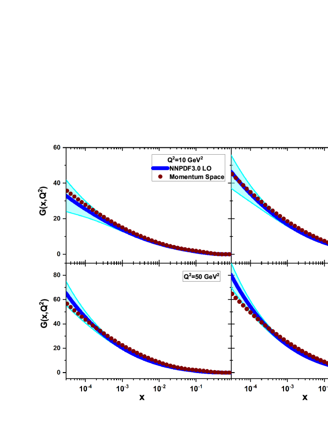
The results for the gluon distribution function (i.e. Eq.(18)) in the momentum space are presented in Fig.4 and compared with the NNPDF3.0LO gluon structure function [32] as accompanied with total errors. Calculations have been performed without considering the rescaling variable of $x$. As can be seen in this figure (i.e., Fig.4), the results are comparable with the NNPDF3.0LO for $Q^{2}=10,20,50$, and $100~{}\mathrm{GeV}^{2}$ in a wide range of $x$. Notably, the values of the gluon distribution function increase as $x$ decreases, a trend that is in harmony with the expectations of pQCD. The results of $G(x,Q^{2})$ based on the momentum space show very good agreement with the NNPDF3.0LO gluon structure function for moderate $Q^{2}$ in the range $10^{-5}{\leq}x{\leq}1$.

In summary, our calculation of the reduced cross section in momentum space employs the Block-Durand-Ha parameterization for the proton structure function $F_{2}(x,Q^{2})$ and the LO longitudinal structure function $F_{L}(x,Q^{2})$, as proposed by Boroun and Ha, utilizing Laplace transform techniques. We have benchmarked our reduced cross section results against the H1 data and extrapolated them into the LHeC domain. Furthermore, the ratio $F_{L2}(x,Q^{2})$ derived from our analysis is compared with both the H1 data and the CDP bounds, showing consistency. Lastly, our evaluation of the gluon distribution functions $G(x,Q^{2})$ in momentum space corroborates the NNPDF3.0LO gluon distribution functions for moderate $Q^{2}$ values within the range $10^{-5}{\leq}x{\leq}1$.

Phuoc Ha would like to thank Professor Loyal Durand for useful comments and invaluable support.

Let us start with the series in Eq. (13):

$\displaystyle S(v)=\sum_{k=1}^{\infty}\frac{k}{(k+1)^{2}-3(k+1)+4}e^{-(k+1)v}=\sum_{m=1}^{\infty}\frac{m-1}{m^{2}-3m+4}e^{-mv}.$

(19)

For large $m$, the terms in the series behave as $e^{-mv}/m$. Noting that

$\displaystyle\sum_{m=1}^{\infty}\frac{e^{-mv}}{m}=-\ln{(1-e^{-v})}=-\ln{(1-x)},$

(20)

we can subtract this series from Eq.(19) to get a series that converges as $e^{-mv}/m^{2}$, so converges even as $v\rightarrow 0$, and add it back in as $-\ln{(1-e^{-v})}$. This gives

$\displaystyle S(v)=\sum_{m=1}^{\infty}\frac{2m-4}{m(m^{2}-3m+4)}e^{-mv}-\ln{(1-e^{-v})}.$

(21)

The result also shows explicitly the divergence for $x=-e^{-v}\rightarrow 1$ or $v\rightarrow 0$.

Let us denote

$\displaystyle S_{\rm mod}(v)=\sum_{m=1}^{\infty}\frac{2m-4}{m(m^{2}-3m+4)}e^{-mv}.$

(22)

We can further improve the convergence of the series $S_{\rm mod}(v)$ by subtracting the asymptotic series for $m$ large and adding it back in as the dilogarithm ${\rm Li}_{2}(e^{-v})=\sum_{m=1}^{\infty}e^{-mv}/m^{2}$ . This gives a series in which the remainder, after $M$ terms, is of order $1/M^{2}$

$\displaystyle S_{\rm mod}(v)=\sum_{m=1}^{\infty}\bigg{[}\frac{2m-4}{m(m^{2}-3m+4)}-\frac{2}{m^{2}}\bigg{]}e^{-mv}+{\rm Li}_{2}(e^{-v}).$

(23)

In Fig. 5, we show the plots of $S(\upsilon)$ and $S_{\rm mod}(\upsilon)$, given by Eq. (21) and Eq. (23), respectively, in a wide range of $\upsilon$. In both plots, the maximum of $m$ in the series is chosen to be $M=1000$ with a point wise accuracy $\sim 1/10^{6}$. For present purposes value $M\sim 50$ with accuracy $1/10^{4}$ or better is sufficient.

References

- (1) H1 Collab. (C.Adloff et al.), Eur.Phys.J.C 21 (2001) 33.
- (2) S.Schmitt, Workshop on EW and BSM physics at the EIC(2020); K.Lipka, Standard model at the LHC (2013).
- (3) J. Abelleira Fernandez, et al. [LHeC Collaboration], J. Phys. G 39 (2012) 075001.
- (4) P.Agostini et al. [LHeC Collaboration and FCC-he Study Group], J. Phys. G: Nucl. Part. Phys. 48 (2021) 110501.
- (5) M. Klein, arXiv:1802 .04317[hep -ph].
- (6) M. Klein, Ann. Phys. 528 (2016) 138.
- (7) N. Armesto, et al., Phys. Rev. D 100 (2019) 074022.
- (8) G.R.Boroun and B.Rezaei, Phys. Lett. B 816 (2021) 136274.
- (9) N. N. Nikolaev and B. G. Zakharov, Phys. Lett. B 332 (1994) 184.
- (10) N. N. Nikolaev and B. G. Zakharov, Z. Phys. C 49 (1991) 607.
- (11) N. N. Nikolaev and B. G. Zakharov, Z. Phys. C 53 (1992) 331.
- (12) K. Golec-Biernat and M. Wsthoff, Phys. Rev. D 59 (1999) 014017; Phys. Rev. D 60 (1999) 114023.
- (13) J. Bartels, K. Golec-Biernat and H. Kowalski, Phys. Rev. D 66 (2002) 014001.
- (14) G. Cvetic, D. Schildknecht, B. Surrow and M. Tentyukov, Eur. Phys. J. C 20 (2001) 77.
- (15) M. Kuroda and D. Schildknecht, Phys. Lett. B 618 (2005) 84; Phys. Lett. B 670 (2008) 129; Phys. Rev. D 85 (2012) 094001; J. Mod. Phys. A 31 (2016) 1650157.
- (16) G.R.Boroun, M. Kuroda and D. Schildknecht, arXiv[hep-ph]:2206.05672.
- (17) D. Schildknecht and M. Tentyukov, arXiv[hep-ph]:0203028.
- (18) C. Ewerz, A. von Manteuffel and O. Nachtmann, Phys.Rev.D 77 (2008) 074022.
- (19) C. Ewerz, A. von Manteuffel, O. Nachtmann and A. Schoning, Phys.lett.B 720 (2013) 181.
- (20) C. Ewerz, O. Nachtmann, Phys.Lett.B 648 (2007) 279.
- (21) B.Rezaei and G.R.Boroun, Phys.Rev.C 101, (2020) 045202.
- (22) M. Niedziela and M. Praszalowicz, Acta Physica Polonica B 46 (2015) 2018.
- (23) G.R.Boroun and B.Rezaei, Phys.Rev.C 103, (2021) 065202; Nucl.Phys.A 990 (2019) 244.
- (24) G.R.Boroun, Eur.Phys.J.A 57 (2021) 219; Phys.Rev.D 109 (2024) 054012.
- (25) M. M. Block, L. Durand and P. Ha, Phys.Rev.D 89 (2014) 094027.
- (26) G.R.Boroun and P.Ha, Phys.Rev.D 109 (2024) 094037.
- (27) Martin M. Block, Loyal Durand and Douglas W. McKay, Phys.Rev.D 79 (2009) 014031.
- (28) Martin M. Block, Loyal Durand, Phuoc Ha and Douglas W. McKay, Phys.Rev.D 83 (2011) 054009.
- (29) Martin M. Block, Loyal Durand, Phuoc Ha and Douglas W. McKay, Phys.Rev.D 84 (2011) 094010.
- (30) Martin M. Block, Loyal Durand, Phuoc Ha and Douglas W. McKay, Phys.Rev.D 88 (2013) 014006.
- (31) H1 Collab. (V. Andreev et al.), Eur.Phys.J.C 74 (2014) 2814.
- (32) NNPDF Collaboration (Richard D. Ball et al.), JHEP 04 (2015) 040.
- (33) L.P. Kaptari, et al., Phys.Rev.D 99 (2019) 096019.
- (34) M.A.G.Aivazis et al., Phys.Rev.D 50 (1994) 3102.
- (35) T. Lappi, H. Mantysaari, H. Paukkunen, and M.Tevio, Eur. Phys. J. C 84 (2024) 84.