ReDFeat: Recoupling Detection and Description for Multimodal Feature Learning

The joint detection and description framework of local feature learning aims to employ DNN to extract a dense descriptor map $\boldsymbol{D}(\boldsymbol{\Omega_{a}},\boldsymbol{\Omega_{e}})\in\mathbb{R}^{H\times W\times C}$ and a detection score map $\boldsymbol{S}(\boldsymbol{\Omega_{a}},\boldsymbol{\Omega_{e}},\boldsymbol{\Omega_{d}})\in\mathbb{R}^{H\times W}$ for an input image $\boldsymbol{I}\in\mathbb{R}^{H\times W}$, where $\boldsymbol{\Omega_{a}}$, $\boldsymbol{\Omega_{e}}$, $\boldsymbol{\Omega_{d}}$ denote the parameters of adapter, encoder and detector, respectively. Let $\{i,i^{\prime}\}$ represent a correspondence in a pair of overlapping images $\boldsymbol{I}$ and $\boldsymbol{I}^{\prime}$, $\boldsymbol{d}_{i}\in\boldsymbol{D}$ represent the descriptor of $i$th point with detected probability $s_{i}\in\boldsymbol{S}$.

To constrain the learning of an individual descriptor $\boldsymbol{d}_{i}$, a matching risk function $\mathcal{R}_{i}(\boldsymbol{d}_{i};\boldsymbol{D},\boldsymbol{D}^{\prime})$ is constructed within descriptor maps $\boldsymbol{D}$ and $\boldsymbol{D}^{\prime}$. Since the reliability of the descriptor can be estimated by $\mathcal{R}_{i}(\boldsymbol{d}_{i};\boldsymbol{D},\boldsymbol{D}^{\prime})$ to some extent, many related works couple the corresponding detection scores $s_{i}$ and $s_{i^{\prime}}$ to guide the optimization of $\mathcal{R}_{i}(\boldsymbol{d}_{i};\boldsymbol{D},\boldsymbol{D}^{\prime})$ in a general loss:

where $\mathbb{E}(\cdotB)$ denotes the expectation calculation (averaging in batch). While the descriptors with larger detection score $s_{i}$ would play more important roles during the optimization, the detection scores of points with large $\mathcal{R}(\boldsymbol{d}_{i};\boldsymbol{D},\boldsymbol{D}^{\prime})$ would tend to be zeros. In this way, problems come up: firstly, the zero detection score map is one of a local minimum of this loss, which is not our desire. Secondly, the hard descriptors with large $\mathcal{R}(\boldsymbol{d}_{i};\boldsymbol{D},\boldsymbol{D}^{\prime})$ are the key for improvement, so they deserve more attention instead of being treated as distractors. The two problems are magnified in multimodal feature learning, in which the correspondences suffer from the extreme variance of imaging.

Although D2-Net [12] and CMMNet [9] conduct normalization onto detection score $s$ so that $\boldsymbol{S}=0$ would not be the minimum of the loss, the normalization breaks the convexity of detection and the balance between the learning of detection and description would be hard to hold, which finally leads to failed optimization. Reliability loss of R2D2 [27] also contains a term similar to Eqn. (1), which would suffer from the first problem mentioned before. The failures of CMMNet and R2D2 prove our hypothesis as shown in Section VI. Moreover, the formulation of probabilistic matching loss introduced in ReinforcedPoint [6] and DISK [34] is also similar to Eqn. (1), so it is likely to get stuck in the two problems. Therefore, we devote ourselves to recoupling detection and description in a more elaborated way for better training.

The basic constraints of detection and description should be determined before coupling them. To satisfy the nearest neighbor matching principle, the distance between an anchor and its nearest non-matching neighbor should be maximized, while the distance to its correspondence should be minimized. Therefore, we sample $N$ pairs of corresponding descriptors $\{\boldsymbol{d}_{i},\boldsymbol{d}_{i^{\prime}}\}$ and their detection scores $\{s_{i},s_{i^{\prime}}\}$. The set of samples is denoted by $\{\boldsymbol{D}_{N},\boldsymbol{D}^{\prime}_{N}\}$. For a pair corresponding cross-modal descriptors $\{\boldsymbol{d}_{i},\boldsymbol{d}_{i^{\prime}}\}$, we mine two intra-modal nearest non-matching neighbor $\{\boldsymbol{d}_{j},\boldsymbol{d}_{k}\}$ and two inter-modal non-matching neighbor $\{\boldsymbol{d}_{m},\boldsymbol{d}_{n}\}$ in $\{\boldsymbol{d}_{i},\boldsymbol{d}_{i^{\prime}}\}$ as:

where $\theta(\boldsymbol{d}_{i},\boldsymbol{d}_{j})=\text{acos}(\boldsymbol{d}_{i}^{T}\boldsymbol{d}_{j})$ is the angular distance. Although the nearest neighbor matching request distinction between an anchor and its inter-modal nearest neighbor, we believe maximizing $\theta(\boldsymbol{d}_{i},\boldsymbol{d}_{n})$ and $\theta(\boldsymbol{d}_{i},\boldsymbol{d}_{m})$ in the meantime is hazardous for acquiring the modal invariance. Thus we tend to maximize $\text{max}\{\theta(\boldsymbol{d}_{i},\boldsymbol{d}_{n}),\theta(\boldsymbol{d}_{i},\boldsymbol{d}_{m}))\}$, $\theta(\boldsymbol{d}_{i},\boldsymbol{d}_{k})$ and $\theta(\boldsymbol{d}_{i},\boldsymbol{d}_{j})$, while minimizing $\theta(\boldsymbol{d}_{i},\boldsymbol{d}_{i^{\prime}})$ in contrastive learning behavior. As a result, our basic loss function of description $\mathcal{L}_{\text{desc-B}}$ is:

The angular distance is employed for distance measure because it could balance the optimization of matching and non-matching pairs [22]. Moreover, the quadratic matching risk makes the hard samples obtain larger gradients to be optimized. In this way, $\mathcal{L}_{\text{desc-b}}$ is expected to increase the cross-modal robustness of descriptors.

As mentioned above, repeatability and local peaking should be the primary properties of detection. To guarantee the repeatability, the detection score $\boldsymbol{S}$ of the first image should be similar to the warped $\boldsymbol{S}^{\prime}_{w}$ of the other image. Moreover, the detection score should be salient so that a unique point can be extracted in a local area. Thus, we follow R2D2 [27] to primarily constrain the detection with basic repeatability loss $\mathcal{L}_{\text{rep-B}}$ and peaking loss $\mathcal{L}_{\text{peak-B}}$ as:

where $p$ is a flattened patch of coordinate, which is extracted on full coordinate $\{1,\dots,H\}\times\{1,\dots,W\}$ by shifted windows with kernel size of $17\times 17$ and stride of $8$; $\boldsymbol{S}[p]\in\mathbb{R}^{256}$ denotes the flattened and normalized vector of detection score, which is indexed by $p$; AP and MP denote the average pooling and the max pooling with kernel size of $17\times 17$ and stride of $1$, respectively. Note that, the kernel size and the strides are all adopted from R2D2 empirically.

Successes of the related works [12, 27, 34] suggest that coupling detection and description can improve the feature learning, however, inappropriate coupling strategies bring up problems as mentioned in Section III-A. To tackle problems, we recouple them with a mutual weighting strategy, in which the gradients of weights are ‘stopped’ as illustrated in Fig. 1. Specifically, we again sample $N$ pair of corresponding descriptors $\{\boldsymbol{d}_{i},\boldsymbol{d}_{i^{\prime}}\}$ and their detection scores $\{s_{i},s_{i^{\prime}}\}$. For detection, a weight ${a}(\mathcal{R}(\boldsymbol{d}_{i};\boldsymbol{D},\boldsymbol{D}^{\prime})$ that is negatively correlated to matching risk $\mathcal{R}(\boldsymbol{d}_{i};\boldsymbol{D}_{N},\boldsymbol{D}^{\prime}_{N})$ would encourage the more reliable descriptor to be detected in a higher probability. Furthermore, learning from the handcrafted cross-modal features which focus on modal-invariant texture extraction, we introduce an edge-based prior $\boldsymbol{M}(\boldsymbol{I})$ to prevent the interest points from laying on smooth areas. So the recoupled peaking loss $\mathcal{L}_{\text{peak-R}}$ can be formulated as:

where $[\cdot]_{+}$ denotes the rectified linear unit (ReLU); $\triangleq$ denotes the ‘stop gradient equality’; the edge of image $\boldsymbol{I}$ is computed as $\|\nabla^{2}\boldsymbol{I}\|$ with Laplacian operator. The weights ${a}(\mathcal{R}(\boldsymbol{d}_{i};\boldsymbol{D},\boldsymbol{D}^{\prime})$ and $\boldsymbol{M}(\boldsymbol{I})$ are visualized in Fig. 2 (b) and (c), respectively.

There are several key differences between our peaking constraints and previous works. Firstly, the recoupling weight $a(\mathcal{R}(\boldsymbol{d}_{i};\boldsymbol{D},\boldsymbol{D}^{\prime}))$ is detached from back propagation, which would not directly affect the learning of description [12, 9, 27, 34]. Secondly, $a(\mathcal{R}(\boldsymbol{d}_{i};\boldsymbol{D},\boldsymbol{D}^{\prime}))$ only constrains the peaking of the detection, which would not suppress any detected probability of hard descriptors with large $\mathcal{R}(\boldsymbol{d}_{i};\boldsymbol{D},\boldsymbol{D}^{\prime})$ and solve the problems mentioned above [12, 9, 27, 34]. Thirdly, edge-based priori $\boldsymbol{M}(\boldsymbol{I})$ is introduced to balance the peaking constraint, instead of forcing the model to detect corners or edges [11, 20, 4]. Moreover, the weights are normalized by the expectation dynamically, so the weights would not be zeros and keep functioning. In this way, while the detection turns explainable and reliable, it can be more stably trained without risks of falling into sub-optimum, i.e., trivial solution.

Multimodal sensors may display the same object in totally different forms, which means requesting repeatability in such areas is exactly irrational. Thus, the repeatability also needs guides from the description. For two corresponding patches of detection score, we compute the average cosine similarity of their descriptors to estimate the local similarity. Then, the local similarity is used as a weight to modulate the recoupled repeatability loss as:

where $\boldsymbol{D}_{w}^{\prime}$ denotes the warped dense descriptors. Note that the detached $b(p;\boldsymbol{D},\boldsymbol{D}_{w}^{\prime})$ would also not affect the optimization of description. And $\boldsymbol{D}[p[i]]^{T}\boldsymbol{D}^{\prime}_{w}[p[i]]$ in the weight $b(p;\boldsymbol{D},\boldsymbol{D}_{w}^{\prime})$ is visualized in Fig. 2 (e).

As discussed before, since the flattening and peaking of detection are safely defined and hold a balance in the recoulped peaking loss, the detection would slip into trivial solution, e.g., zeros. Therefore, it is worth recoupling the detection to the description. In other words, the matching risk can be weighted with the detection score so that the descriptors with high detected probability would attract more attention in the optimization. The recoupled description loss with detached weights can be formulated as:

where $c(s_{i},s_{i}^{\prime})$ is shown in Fig. 1 (f).

Finally, the total loss function of our RedFeat can be formulated in the sum of Eqns. (9), (12) and (14) with only one hyperparameter $\lambda$:

While the weights ${a}(\mathcal{R}(\boldsymbol{d}_{i};\boldsymbol{D},\boldsymbol{D}^{\prime})$ and $b(p;\boldsymbol{D},\boldsymbol{D}_{w}^{\prime})$ are generated by description and recoulped to the detection, the weight $c(s_{i},s_{i}^{\prime})$ takes a converse effect in the loss. This loss based on the mutual weighting strategy would stabilize and boost the feature learning.

Architecture. Most joint detection and description methods share similar architectures which include an encoder and a detector. R2D2 proposes a lightweight encoder that contains only $9$ convolution layers and a naive linear detector to output 128-dimensional dense descriptors and a score map, which is cheap in time and memory. Therefore, we adopt this architecture as our raw architecture. The $6$ shallow layers are divided as the adapter that is unshared for eliminating the variance of modals. The raw encoder in our architecture consists of the last $3$ convolutional layers and the raw detector keeps the same with R2D2. Note that, the encoder and detector are weight sharing.

Super Detector. Our recoupling constraints mainly embrace the detection. limited by the small receptive field, the raw linear detector cannot capture the neighborhood and global information to fulfill peaking loss. Therefore, we propose a super detector, which has two branches like R2D2. One branch is the raw detector $\theta_{d0}$ that models the prior probability $p({kp}_{i}|\boldsymbol{d}_{i})$ that the point $i$ is a keypoint as $p({kp}_{i}|\boldsymbol{d}_{i})=\text{Sigmoid}(\theta_{d0}(\boldsymbol{d}_{i}))$; The structure of the other branch needs to model the conditional probability $p(dp_{i}|\boldsymbol{D},kp_{i})$ that a keypoint can be detected globally.

Since $p({dp}_{i}|\boldsymbol{D},{kp}_{i})$ is related to global information, the branch should possess a larger receptive field by stacking more convolutional layers. Moreover, the score of the detected point should be the local maximum, so we propose learnable non-maximum suppression layer (LNMS) as shown in Fig. 3. In the LMNS, features are firstly transformed by a learnable convolutional layer. Then, local maximums in the transformed feature map are detected by the local softmax operation, i.e., Eqn. (18). At last, statistical maximums in batch and channel are further mined by BN and IN with ReLU. Briefly, for an input feature map $\boldsymbol{x}$, the forward propagation in LNMS can be described as:

where AP3 denotes average pooling with a kernel size of $3$. BN and IN represent batch normalization and instance normalization, respectively. Finally, the branch is constructed by cascading convolutional layers and several LNMS as shown in Fig. 3, and it outputs a two-channel feature. After channel softmax activation, the first channel in the final feature map is maintained as $p({dp}_{i}|\boldsymbol{D},{kp}_{i})$. The posterior probability $p({kp}_{i}|\boldsymbol{D},{dp}_{i})$ that the detected point is an interest point, i.e., $s_{i}$, can be approximately computed as $p({kp}_{i}|\boldsymbol{d}_{i})p({dp}_{i}|\boldsymbol{D},{kp}_{i})$.

VIS-NIR. Visible and near-infrared (NIR) image pairs in the average size of $983\times 686$ are collected from the RGB-NIR scene dataset [7]. The dataset covers various scenes, including country, field, forest, indoor, mountain, old building, street, urban, and water. And most image pairs are photographed in special conditions and can be well registered. We randomly split the images from $9$ scenes into the training set and the test set with a ratio of $3:1$, which results in a training set of $345$ pairs of images. The ground truths of the test set are manually validated and filtered for more reliable evaluation. Finally, there are $128$ pairs of images left in the test set.

VIS-IR. We collect roughly registered 265 pairs of visible and long-wave infrared (IR) images in the average size of $533\times 321$. $44$ static image pairs from RGB-LWIR [3] are mainly shot on buildings during the day. The other $221$ pairs of video frames come from RoadScene [39], in which more complex objects, e.g., cars and people, are captured both day and night. We randomly select $47$ images as the test set and leave the rest as the training set. Since the overlapping image pairs cannot be registered with the homography matrix due to the greatly varying depth of objects, we manually mark about $16$ landmarks per image pair for reprojection error estimation.

VIS-SAR. Optical-SAR [37] provides aligned gray level and synthetic aperture radar image pairs in the uniform size of $512\times 512$, which are remotely sensed by the satellite and cover field and town scenes. There are 2011 and 424 image pairs in the training set and test set, respectively. The dataset and its split are gathered into our benchmark without changes. Note that, it is hard to validate the ground truth or label landmarks for this subset due to the fuzziness of SAR images.

Random Transform. Cross-modal features should carry both geometric and modal invariance. Thus, we generate homography transforms $\boldsymbol{H}$ by cascading random perspective with distortion scale $[0,0.2]$, random rotation $[-10^{\circ},10^{\circ}]$ and random scaling $[0.8,1.0]$. And then, the transforms $\boldsymbol{H}$ are conducted on the aligned raw test set to generate the warped test set.

Feature Matching. To generate sufficient matches, the detected keypoints should be repeatable and the extracted descriptors should be robust. To evaluate the repeatability of the keypoints, we compute the number of correspondences (Corres) of image pairs and the repeatable rate (RR), i.e., the ratio of the number of correspondences over the detected keypoints. Furthermore, we match the descriptors with the bidirectional nearest neighbor matching and calculate the number of correct matches. Following the definition in [11, 27], we report matching score (MS), that the ratio of the number of correct matches over the number of the detected keypoints in the overlap, to evaluate the robustness of descriptors. Note that, the metrics are validated at different thresholds of pixels. And RR and MS are computed symmetrically across the pair of images and averaged.

Image Registration. The image registration is the destination of local feature learning. The matched features are used to estimate homography transform $\boldsymbol{H}^{\prime}$ with RanSAC from OpenCV libraries, where the reprojection threshold is set to $10$ pixels and the iterations to $100$K. Since the ground-truth transform $\boldsymbol{H}$ is provided, we compute the reprojection error $RE_{H}$ as:

where $\boldsymbol{H}[:]$ denotes the flatten vector of $\boldsymbol{H}$. However, this metric would be not indicative for VIS-IR subset, because the raw test image pairs are not well aligned. Therefore, we introduce another method to estimate reprojection error with the landmarks as:

where $\boldsymbol{M}$ and $\boldsymbol{M}^{\prime}$ denote the set of landmarks $\boldsymbol{m}$ on two images; $\tau(\boldsymbol{m}_{i},\boldsymbol{H}^{\prime})$ represents the reprojected point of $\boldsymbol{m}_{i}$. The registration is successful, if RE is smaller than a threshold. The successfully registered images (SR) are counted and the successful registration rate (SRR) is calculated on each subset.

We implement our ReDFeat in PyTorch [25] and Kornia [28]. The training data in a size of $192\times 192$ is achieved by cropping, normalization and random perspective transform mentioned above. The network is trained in about 10000 iterations with a batch size of 2 on an NVIDIA RTX3090 GPU. Adam optimizer [17] with weight decay of $0.0005$ is employed to optimize the loss. Its learning rate is initialized at $0.001$ and decays to $0$ at the last epoch. The last checkpoint of training would be used for evaluation.

Our ReDFeat is compared to several counterparts in our benchmark, including SIFT [21], RIFT [18], DOG+HN [23], R2D2 [27] and CMMNet [9]. SIFT and RIFT are extracted with the open-source codes and default settings. HardNet and R2D2, which are deep learning features for visible images, are modified to multimodal scenario by specializing parameters of the first $6$ convolutional layers for individual modal images. CMMNet, which is not open-source, is implemented on the codebase of D2Net [12].

Training Stability. Since the training stability is the key problem that our recoupling strategy aims to tackle, we try to train the CMMNet, R2D2 and our method from scratch or pre-trained models to confirm our motivation. CMMNet adopts the VGG-16 pre-trained on ImageNet as the initialization. For comparison, we use the official pre-trained model for visible images to initialize R2D2 for cross-modal images. For ReDFeat, we just employ self-supervised learning [11], which is fed with augmented visible images, to obtain a pre-trained model. The mean number of correct matches and MS of $1024$ keypoints on VIS-IR subset are shown in Table II. As we can see, CMMNet and R2D2 fail to learn discriminative features without pre-trained models, because the joint optimization of their naive coupled constraints is ill-posed. By contrast, our ReDFeat can be readily trained from scratch while also achieving a tiny improvement from the self-supervised pre-trained, which demonstrates the solidity of our formulation. Therefore, while we keep initializing the training of CMMNet and R2D2 with pre-trained models in subsequent experiments, our ReDFeat would be always trained from scratch.

Impact of $\lambda$. The weight of $\mathcal{L}_{\text{rep-R}}$, $\lambda$, is the only hyperparameter of ReDFeat, which plays a crucial role in balancing detection and description in our recoupling strategy. To investigate the impact of $\lambda$, we train ReDFeat with different $\lambda$ values and report relevant metrics of $1024$ keypoints on VIS-IR in Table III. Totally, $\lambda$ lager than $8$ brings out desirable registration performance that the community focuses on. It demonstrates that the repeatability constrained by $\mathcal{L}_{\text{rep-R}}$ and weighted by $\lambda$ impose a strong impact on the registration performance. However, the repeatability not only forces the detection to be similar but also narrows the gap between two descriptor maps and decreases the distinction of descriptors, which can be proved by the decrease of the correct matches. Therefore, the image registration performance peaks at $\lambda=8$ and the setting would be kept in subsequent experiments.

Proposed Components. We propose three novel modifications: \scriptsize1⃝ basic constraints, \scriptsize2⃝ recoupled constraints and \scriptsize3⃝ new networks for multimodal feature learning. To evaluate the efficiency of our proposals, we choose R2D2, which provides the raw network architecture for losses, as the baseline, and the modifications are successively executed in this framework. As we can see in Table IV, our basic loss is more suitable for multimodal feature learning and remarkably improves the baseline on all metrics. The recoupled constraints obtain further improvements on feature matching tasks, while the registration performance is comparable to the former. After the new network, i.e., Super Detector, is equipped, state-of-the-art results are achieved. So far, the proposed components are proved to take positive effects.

To gain an insight into the impacts of our proposals, we visualize the detection score maps, what we discuss throughout our formulation, under different configurations in Fig. 4. As shown in the second and the third columns of images, while the local peaking loss guides R2D2 to generate discrete detection score, it leads to bulks of detection basic constraints. It can be explained that $\lambda=8$ moderates the impact of local peaking in basic constraints. These lumped detected features intend to repeat and be matched within an acceptable error so that the matching performance is improved. After recoupling the constraints, the edge-based priori makes the detection gather in areas with rich textures, which is expected to obtain further improvements. Finally, the Super Detector equipped with learnable local non-maximum suppression blocks introduces a strong inductive bias to discretize the detection score. The discrete detection score must tighten weighted description loss and repeatability loss, which is believed to help the joint learning and improve the accuracy of keypoint location.

The feature matching performance of 1024 keypoints of SIFT, RIFT, HN, R2D2, CMMNet, and our RedFeat on three subsets is quantified in Fig. 5, in which RR and MS are selected as the primary metrics and calculated at varying thresholds. As we can see, we achieve the state-of-the-art RR and MS at all thresholds on three subsets, which demonstrates that we obtain more robust descriptors while detecting more precise and repeatable keypoints. As for MS, we gain large margins on all subsets at varying thresholds. Especially on the most challenging subset, VIS-SAR, our MS seems to be several times higher than the second place CMMNet. It is worth mentioning that R2D2 employing pre-trained models for initialization still fails to optimize the description on VIS-SAR, which confirms the significance of our recoupling strategy.

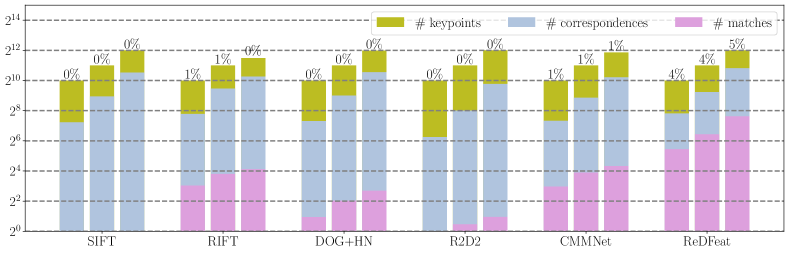
More quantitative performance of 1024, 2048 and 4096 keypoints at a threshold of 3px is shown in Fig. 6. The matching score that is key index for feature matching performance is deliberately highlighted on the bars. Except for the number of correspondences on VIS-IR and VIS-SAR, our ReDFeat achieve the best scores on all metrics at 3px. Note that, the handcrafted local-maximums-searching-based detector might fail to extract large numbers of keypoints for some image pairs, which demonstrates the superiority and the flexibility of the learnable detection.

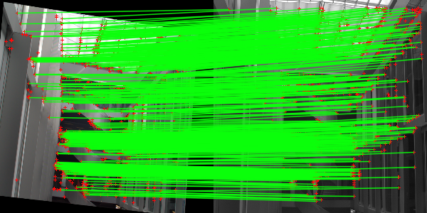
Qualitative performance is shown in Fig. 7. Compared to R2D2 and CMMNet, our detected points seem to be more rationally distributed in the textured area, i.e., intensely but not too intensely. However, traditional detectors employed by SIFT, RIFT, and DOG-HN seemingly generate more interpretable results that strictly attach to the edges or corners. Especially, RIFT detects scattered corner points, which are proved by RR shown in Fig. 5 and the number of correspondences shown in Fig. 6, in not so salient regions. The weakness of the deep learning detector can be attributed to the flaws of the training set, which cannot provide strict correspondences so that the keypoints are not precisely located. Despite the advantages of traditional detectors, the deep learning one-stage and two-stage methods show the superiority of deep learning on the feature description. In our method that the description and detection are mutually guided in our recoupling strategy, the hard descriptors are better optimized, which makes significant progress in matching performance.

Successful registration rates of 1024 keypoints of those algorithms are drawn in Fig. 8. Note that, we use two measures of projection error (RE) on the three subsets according to the quality of the ground truths. Nevertheless, our ReDFeat obtains more successfully registered images pairs in each case. And the margin is more prominent on VIS-SAR that is the most challenging. Moreover, the weak performance of CMMNet on VIS-NIR highlights the important of keypoint location, i.e., the registration performance depends on MS at low thresholds. The problem is well tackled by recoupled constraints and Super Detector in our method, as proved in ablation study.

The distributions of reprojection errors of 1024, 2048 and 4096 keypoints are illustrated in Fig. 9. Except on the VIS-NIR with $2048$ and $4096$ keypoints, our method achieves the most SR and the lowest mean RE. Particularly, while greatly boosting SR on VIS-SAR, our method gets the mostly precise image registration performance. As for the tiny disparity of RE among SIFT, DOG-HN, and ReDFeat on VIS-NIR, it can be explained by the small discrepancy between visible and near-infrared images and the accuracy of handcrafted keypoint location as mentioned above.

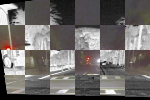
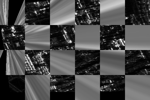
Some examples, in which only our ReDFeat succeeds, are shown in Fig. 10. Although RIFT, R2D2 and CMMNet estimate approximate transforms in some cases from VIS-NIR and VIS-IR, the accuracy of registration does not meet the expectations. On samples of VIS-SAR, the other alternatives even fail to receive a rough result, which is consistent with the feature matching performance. Generally, with the help of recoupled constraints and Super Detector, our method can learn robust cross-modal features that indeed boost the performance of cross-modal image registration.

Time consumption is important for feature extraction. Because SIFT, RIFT, DOG+HN and CMMNet employ handcrafted detectors, their computation complexities are hard to calculate. And we just report the average runtime in three test sets in Table V. All of them are implemented in Python, except RIFT which is implemented in Matlab. All methods are run on an Intel Xeon Silver 4210R CPU and an NVIDIA RTX3090 GPU. As we can see, R2D2 consumes the least time to extract features for each image. And benefiting from the parallel computation on GPU, its runtime is not sensitive to the image size. Because of the complex operations in Super Detector, ReDFeat takes more time to finish the extraction. However, the improvements of our method are believed to be worth the increased runtime. All methods seem to be time-consuming except SIFT which takes the same order of magnitude of time as R2D2 and ReDFeat. Generally, we significantly improve the performance of features with few extra costs.

References

- [1] Cristhian Aguilera, Fernando Barrera, Felipe Lumbreras, Angel D Sappa, and Ricardo Toledo. Multispectral image feature points. J. Sens., 12(9):12661–12672, 2012.
- [2] Cristhian A Aguilera, Angel D Sappa, Cristhian Aguilera, and Ricardo Toledo. Cross-spectral local descriptors via quadruplet network. J. Sens., 17(4):873–887, 2017.
- [3] Cristhian A Aguilera, Angel D Sappa, and Ricardo Toledo. Lghd: A feature descriptor for matching across non-linear intensity variations. In Proc. IEEE Int. Conf. Image Process., pages 178–181, 2015.
- [4] Axel Barroso-Laguna, Edgar Riba, Daniel Ponsa, and Krystian Mikolajczyk. Key. net: Keypoint detection by handcrafted and learned cnn filters. In Proc. IEEE Conf. Comput. Vis. Pattern Recognit., pages 5836–5844, 2019.
- [5] Herbert Bay, Tinne Tuytelaars, and Luc Van Gool. Surf: Speeded up robust features. In Proc. Europ. Conf. Comput. Vis., pages 404–417, 2006.
- [6] Aritra Bhowmik, Stefan Gumhold, Carsten Rother, and Eric Brachmann. Reinforced feature points: Optimizing feature detection and description for a high-level task. In Proc. IEEE Conf. Comput. Vis. Pattern Recognit., pages 4948–4957, 2020.
- [7] Matthew Brown and Sabine Süsstrunk. Multi-spectral sift for scene category recognition. In Proc. IEEE Conf. Comput. Vis. Pattern Recognit., pages 177–184, 2011.
- [8] Bingyi Cao, Andre Araujo, and Jack Sim. Unifying deep local and global features for image search. In Proc. Europ. Conf. Comput. Vis., pages 726–743, 2020.
- [9] Song Cui, Ailong Ma, Yuting Wan, Yanfei Zhong, Bin Luo, and Miaozhong Xu. Cross-modality image matching network with modality-invariant feature representation for airborne-ground thermal infrared and visible datasets. IEEE Trans. Geosci. Remote Sens., 60:5606414, 2022.
- [10] Song Cui, Ailong Ma, Liangpei Zhang, Miaozhong Xu, and Yanfei Zhong. Map-net: Sar and optical image matching via image-based convolutional network with attention mechanism and spatial pyramid aggregated pooling. IEEE Trans. Geosci. Remote Sens., 60:1000513, 2022.
- [11] Daniel DeTone, Tomasz Malisiewicz, and Andrew Rabinovich. Superpoint: Self-supervised interest point detection and description. In Proc. IEEE Conf. Comput. Vis. Pattern Recognit. Workshops, pages 224–236, 2018.
- [12] Mihai Dusmanu, Ignacio Rocco, Tomas Pajdla, Marc Pollefeys, Josef Sivic, Akihiko Torii, and Torsten Sattler. D2-net: A trainable cnn for joint description and detection of local features. In Proc. IEEE Conf. Comput. Vis. Pattern Recognit., pages 8092–8101, 2019.
- [13] Jianwei Fan, Yan Wu, Ming Li, Wenkai Liang, and Yice Cao. Sar and optical image registration using nonlinear diffusion and phase congruency structural descriptor. IEEE Trans. Geosci. Remote Sens., 56(9):5368–5379, 2018.
- [14] Qiang Fu, Hongshan Yu, Xiaolong Wang, Zhengeng Yang, Yong He, Hong Zhang, and Ajmal Mian. Fast orb-slam without keypoint descriptors. IEEE Trans. Image Process., 31:1433–1446, 2021.
- [15] Xingyu Jiang, Jiayi Ma, Guobao Xiao, Zhenfeng Shao, and Xiaojie Guo. A review of multimodal image matching: Methods and applications. Inf. Fusion, 73:22–71, 2021.
- [16] Yuhe Jin, Dmytro Mishkin, Anastasiia Mishchuk, Jiri Matas, Pascal Fua, Kwang Moo Yi, and Eduard Trulls. Image matching across wide baselines: From paper to practice. Int. J. Comput. Vis., 129(2):517–547, 2021.
- [17] Diederik P Kingma and Jimmy Ba. Adam: A method for stochastic optimization. In Proc. Int. Conf. Learn. Represent., 2014.
- [18] Jiayuan Li, Qingwu Hu, and Mingyao Ai. Rift: Multi-modal image matching based on radiation-invariant feature transform. IEEE Trans. Image Process., 29:3296–3310, 2019.
- [19] Weiquan Liu, Xuelun Shen, Cheng Wang, Zhihong Zhang, Chenglu Wen, and Jonathan Li. H-net: Neural network for cross-domain image patch matching. In Proc. Int. Jt. Conf. Artif. Intell., pages 856–863, 2018.
- [20] Xiaotao Liu, Chen Meng, Fei-Peng Tian, and Wei Feng. Dgd-net: Local descriptor guided keypoint detection network. In Proc. IEEE Int. Conf. Multimed. Expo., pages 1–6, 2021.
- [21] David G Lowe. Distinctive image features from scale-invariant keypoints. Int. J. Comput. Vis., 60(2):91–110, 2004.
- [22] Jiayi Ma and Yuxin Deng. Sdgmnet: Statistic-based dynamic gradient modulation for local descriptor learning. arXiv preprint arXiv:2106.04434, 2021.
- [23] Anastasiya Mishchuk, Dmytro Mishkin, Filip Radenovic, and Jiri Matas. Working hard to know your neighbor’s margins: Local descriptor learning loss. In Adv. Neural Inf. Process. Syst., pages 4829–4840, 2017.
- [24] Raul Mur-Artal, Jose Maria Martinez Montiel, and Juan D Tardos. Orb-slam: a versatile and accurate monocular slam system. IEEE Trans. Robot., 31(5):1147–1163, 2015.
- [25] Adam Paszke, Sam Gross, Francisco Massa, Adam Lerer, James Bradbury, Gregory Chanan, Trevor Killeen, Zeming Lin, Natalia Gimelshein, Luca Antiga, et al. Pytorch: An imperative style, high-performance deep learning library. pages 1–12, 2019.
- [26] Mohammadreza Pourfard, Tahmineh Hosseinian, Roghayeh Saeidi, Sayed Ahmad Motamedi, Mohammad Javad Abdollahifard, Reza Mansoori, and Reza Safabakhsh. Kaze-sar: Sar image registration using kaze detector and modified surf descriptor for tackling speckle noise. IEEE Trans. Geosci. Remote Sens., 60:5207612, 2022.
- [27] Jerome Revaud, Cesar De Souza, Martin Humenberger, and Philippe Weinzaepfel. R2d2: Reliable and repeatable detector and descriptor. pages 1–11, 2019.
- [28] Edgar Riba, Dmytro Mishkin, Daniel Ponsa, Ethan Rublee, and Gary Bradski. Kornia: an open source differentiable computer vision library for pytorch. In Proc. IEEE Winter Conf. Appl. Comput. Vis., pages 3674–3683, 2020.
- [29] Johannes L Schonberger and Jan-Michael Frahm. Structure-from-motion revisited. In Proc. IEEE Conf. Comput. Vis. Pattern Recognit., pages 4104–4113, 2016.
- [30] Amin Sedaghat and Hamid Ebadi. Distinctive order based self-similarity descriptor for multi-sensor remote sensing image matching. J. Photogramm. Remote Sens, 108:62–71, 2015.
- [31] Xuelun Shen, Cheng Wang, Xin Li, Yifan Peng, Zijian He, Chenglu Wen, and Ming Cheng. Learning scale awareness in keypoint extraction and description. Pattern Recognit., 121:108221–108233, 2022.
- [32] Yurun Tian, Axel Barroso Laguna, Tony Ng, Vassileios Balntas, and Krystian Mikolajczyk. Hynet: Learning local descriptor with hybrid similarity measure and triplet loss. In Adv. Neural Inf. Process. Syst., pages 7401–7412, 2020.
- [33] Yurun Tian, Xin Yu, Bin Fan, Fuchao Wu, Huub Heijnen, and Vassileios Balntas. Sosnet: Second order similarity regularization for local descriptor learning. In Proc. IEEE Conf. Comput. Vis. Pattern Recognit., pages 11016–11025, 2019.
- [34] Michał Tyszkiewicz, Pascal Fua, and Eduard Trulls. Disk: Learning local features with policy gradient. pages 14254–14265, 2020.
- [35] Ashish Vaswani, Noam Shazeer, Niki Parmar, Jakob Uszkoreit, Llion Jones, Aidan N Gomez, Łukasz Kaiser, and Illia Polosukhin. Attention is all you need. page 6000–6010, 2017.
- [36] Zihao Wang, Xueyi Li, and Zhen Li. Local representation is not enough: Soft point-wise transformer for descriptor and detector of local features. In Int. Jt. Conf. Artif. Intell., pages 1150–1156, 2021.
- [37] Yuming Xiang, Rongshu Tao, Feng Wang, Hongjian You, and Bing Han. Automatic registration of optical and sar images via improved phase congruency model. IEEE J. Sel. Topics Appl. Earth Observ. Remote Sens., 13:5847–5861, 2020.
- [38] Yuming Xiang, Feng Wang, and Hongjian You. Os-sift: A robust sift-like algorithm for high-resolution optical-to-sar image registration in suburban areas. IEEE Trans. Geosci. Remote Sens., 56(6):3078–3090, 2018.
- [39] Han Xu, Jiayi Ma, Zhuliang Le, Junjun Jiang, and Xiaojie Guo. Fusiondn: A unified densely connected network for image fusion. In Proc. AAAI Conf. Artif. Intell., pages 12484–12491, 2020.
- [40] Hao Zhang, Han Xu, Xin Tian, Junjun Jiang, and Jiayi Ma. Image fusion meets deep learning: A survey and perspective. Inf. Fusion, 76:323–336, 2021.
- [41] Linguang Zhang and Szymon Rusinkiewicz. Learning local descriptors with a cdf-based dynamic soft margin. In Proc. IEEE Int. Conf. Comput. Vis., pages 2969–2978, 2019.
- [42] Zichao Zhang, Torsten Sattler, and Davide Scaramuzza. Reference pose generation for long-term visual localization via learned features and view synthesis. Int. J. Comput. Vis., 129(4):821–844, 2021.