11email: [email protected] 22institutetext: CAS Key Laboratory for Researches in Galaxies and Cosmology, Department of Astronomy, University of Science and Technology of China, Hefei, Anhui 230026, China
22email: [email protected] 33institutetext: School of Astronomy and Space Sciences, University of Science and Technology of China, Hefei, 230026, China 44institutetext: Center for Astrophysics, Guangzhou University, Guangzhou 510006, China 55institutetext: Department of Astronomy, School of Physics, Peking University, 5 Yiheyuan Road, Haidian District, Beijing 100871, China 66institutetext: Kavli Institute of Astronomy and Astrophysics, Peking University, 5 Yiheyuan Road, Haidian District, Beijing 100871, China 77institutetext: National Astronomical Observatories, Chinese Academy of Science, 20A Datun Road, Chaoyang District, Beijing 100101, China 88institutetext: South African Astronomical Observatory, P.O. Box 9, Observatory 7935, Cape Town, South Africa 99institutetext: Astrophysics Science Division, NASA Goddard Space Flight Center, MC 661, Greenbelt, MD 20771, USA 1010institutetext: Steward Observatory, University of Arizona, 933 North Cherry Avenue, Rm. N204, Tucson, AZ 85721-0065, USA 1111institutetext: Astronomical Observatory, University of Warsaw, Al. Ujazdowskie 4, 00-478 Warszawa, Poland 1212institutetext: Max-Planck-Institut für extraterrestrische Physik, Gießenbachstraße 1, 85748 Garching, Germany 1313institutetext: Key Laboratory for the Structure and Evolution of Celestial Objects, Yunnan Observatories, Kunming 650011, China
Recurring tidal disruption events a decade apart in IRAS F01004-2237
Abstract
Context. In theory, recurring tidal disruption events (TDEs) may occur when a close stellar binary encounters a supermassive black hole, if one star is captured and undergoes repeating partial TDEs, or if both stars are tidally disrupted (double TDEs). In addition, independent TDEs may be observed over decades in some special galaxies where the TDE rate is extremely high. Exploring the diversity of recurring TDEs and probing their natures with rich observational data help to understand these mechanisms.
Aims. We report the discovery of a second optical flare that occurred in September 2021 in IRAS F01004-2237, where the first flare occurred in 2010 has been reported, and present a detailed analysis of multi-band data. We aim to understand the nature of the flare and explore the possible causes of the recurring flares.
Methods. We describe our analysis of the position of the flare, the multi-band light curves (LCs), the optical and ultraviolet (UV) spectra, and the X-ray LC and spectra.
Results. The position of the flare coincides with the galaxy centre with a precision of 650 pc. The flare peaks in days with an absolute magnitude of and fades in two years roughly following . It maintains a nearly constant blackbody temperature of 22,000 K in the late time. Its optical and UV spectra show hydrogen and helium broad emission lines with full width at half maxima of 7,000–21,000 km s-1 and He II/H ratio of 0.3–2.3. It shows weak X-ray emission relative to UV emission, with X-ray flares lasting for weeks, during which the spectrum is soft with a power-law index . These characters are consistent with a TDE, ruling out the possibilities of a supernova or an active galactic nuclei flare. With a TDE model, we infer a peak UV luminosity of erg s-1 and an energy budget of erg.
Conclusions. A TDE caused the flare that occurred in 2021. The two optical flares separated by years can be interpreted as repeating partial TDEs, double TDEs, or two independent TDEs. Although no definitive conclusion can be drawn, the partial TDEs interpretation predicts a third flare around 2033, and the independent TDEs interpretation predicts a high TDE rate of yr-1 in F01004-2237, both of which can be tested by future observations.
Key Words.:
XXX, YYY1 Introduction
A tidal disruption event (TDE) occurs when a star wanders close enough to a supermassive black hole (SMBH) that the pericenter distance less than the tidal radius (e.g., Rees 1988):
| (1) |
where and are the radius and the mass of the star, and is the mass of the SMBH. TDEs produce intense electromagnetic radiation converted from the gravitational energy released by the accreted stellar debris, causing bright flares in X-ray, UV, and optical bands peaking in 1–2 months and fading in months to years in centers of galaxies (e.g., Bade et al. 1996; Gezari et al. 2006; van Velzen et al. 2011). In recent years, researchers have begun to study the diversity of the TDE process by considering partial TDEs and double TDEs. Numerical simulations (e.g., Guillochon & Ramirez-Ruiz 2013; Ryu et al. 2020) indicated that the outcome of a star encountering an SMBH depends on the parameter : the star is entirely disrupted when is above a critical value, depending on the stellar structure, and loses a fraction of mass for lower , in which the fraction decreases continuously with decreasing . Theories predicted that partial TDEs are more common than full TDEs (Stone & Metzger 2016; Zhong et al. 2022), and the LCs of partial TDEs decline more rapidly than that of full TDEs in the late-time (Coughlin & Nixon 2019; Miles et al. 2020; Chen & Shen 2021). If the stellar remnant is in an elliptical orbit after a partial TDE, it may be disrupted again after returning to the pericentre, resulting in repeating partial TDEs that are observed as periodic flares. Periodic partial TDEs can result from the encounter of a close binary and an SMBH (Cufari et al. 2022; Liu et al. 2023a). Under the Hills mechanism, in which one star in the binary is captured by the SMBH and the other ejected (e.g., Hills 1988), if the captured star’s pericenter is close enough to the SMBH, or if it is bounced by other existing captured stars into an orbit that facilitate disruption (Bromley et al. 2012), periodic partial TDEs can occur. In addition, simulations show that the encounter of a close binary and an SMBH may lead to various outcomes. One fascinating outcome is double TDEs, where both stars are tidally disrupted (Mandel & Levin 2015). Taking partial disruption into account, the possible outcomes may be even more diverse, and a full TDE and repeating partial TDEs may both occur (Mainetti et al. 2016).
Observationally, verification of a TDE is sometimes challenging because it needs to be distinguished from other TDE analogues (Zabludoff et al. 2021), such as superluminous supernovae (SLSNe, Gal-Yam 2019) and active galactic nuclei (AGN) flares (e.g., Kankare et al. 2017; Oknyansky et al. 2019; Frederick et al. 2019). Characteristics that distinguish TDEs from these analogues include positions consistent with the galactic nuclei, smooth power-law declines in the light curve (LC) roughly following , blackbody continuum in UV/optical bands with constant temperatures of K for hundreds of days, broad emission lines (BELs) with widths remaining relatively broad over months to years, strong He II 4686 BELs and sometimes nitrogen Bowen fluorescence (BF) lines, and soft X-ray emissions with steep spectra (e.g., Saxton et al. 2020; van Velzen et al. 2020; Charalampopoulos et al. 2022). It is generally necessary to assemble a variety of features to classify a flare. However, even so, some flares, for example, CSS100217:102913+404220 (Drake et al. 2011) and ASASSN-18jd (Neustadt et al. 2020), cannot be classified without doubt and are still referred to as ambiguous nuclear transients.
Till now, dozens of spectroscopically confirmed TDEs have been discovered, thanks to large-area high-cadence optical surveys such as the All-Sky Automated Survey for Supernovae (ASASSN, Shappee et al. 2014; Holoien et al. 2016b), the Asteroid Terrestrial-impact Last Alert System (ATLAS, Tonry et al. 2018; Smith et al. 2020), and the Zwicky Transient Facility (ZTF, van Velzen et al. 2021; Hammerstein et al. 2023). With the large number, an accurate rate of optically selected TDE can be measured to be Mpc-3 yr-1, or galaxy-1 yr-1 for galaxies with (Yao et al. 2023). The TDE rate varies greatly among different types of galaxies. For example, the rate in post-starburst galaxies is higher than that in normal galaxies by a factor of several to several tens (French et al. 2016; Graur et al. 2018; Yao et al. 2023). There are many possible explanations for this (see French et al. 2020; Stone et al. 2020, for a review), including SMBH binaries (e.g., Ivanov et al. 2005), central overdensities (e.g., Stone & Metzger 2016; Stone & van Velzen 2016), and others. These explanations facilitate a natural hypothesis that starburst galaxies would also have a high TDE rate. Tadhunter et al. (2017) claimed to verify this hypothesis by finding a TDE candidate in 2010 in IRAS F01004-2237 (hereafter F01004-2237), during monitoring of a sample of 15 dusty starburst galaxies over a decade. However, the result of Tadhunter et al. (2017) is controversial, as Trakhtenbrot et al. (2019) considered the TDE candidate in F01004-2237 as an AGN flare, and we will describe their debates in detail later. The hypothesis of high TDE rate in starburst galaxies has no evidence from other optical surveys, possibly because these TDEs are obscured by dust (Roth et al. 2021). This was supported by the discovery of obscured TDEs via mid-infrared flares such as Arp 299-B AT1 (e.g., Mattila et al. 2018; Reynolds et al. 2022).
Recently, optical rebrightenings or recurring flares have been found in a significant fraction of TDEs (e.g., Jiang et al. 2019; Yao et al. 2023). Some of the recurring flares are suggested to be possibly associated with repeating partial TDEs. Examples are: 1. the two X-ray flares observed in 1990 and 2010 in the Seyfert galaxy IC 3599 (Grupe et al. 1995, 2015; Campana et al. 2015); 2. the 114-day periodic flares in the galaxy ESO 253-G003 repeating for 21 times since the first detection in 2014 (Payne et al. 2021, 2022, 2023); 3. the X-ray transient eRASSt J045650.3-203750 with five gradually weakening flares with time intervals of 200 days (Liu et al. 2023b, 2024); 4. the optical TDE AT 2018fyk and the faint optical flare 3.3 yr after it (Wevers et al. 2019, 2023); 5. the X-ray TDE candidate RX J133157.6-324319.7 in 1993 and the second X-ray flare in 2022 (Hampel et al. 2022; Malyali et al. 2023); 6. the optical TDE AT 2020vdq and the second flare 2.7 yr after it (Hammerstein et al. 2023; Somalwar et al. 2023). 7. the optical TDE AT 2022dbl and the second flare 2 yr after it (Lin et al. 2024). 8. the optical flare AT 2019aalc in a Seyfert galaxy and the second flare 4 yr after it (van Velzen et al. 2024; Milán Veres et al. 2024). Here we do not include events with a double-peak light curve like AT 2019avd (Malyali et al. 2021), because the two peaks can be interpreted as different phases of the same TDE (Chen et al. 2022). The characters of the recurring flares, including periods, luminosities, energy budgets, and SEDs, present colossal diversity. Whether the diversity can be uniformly interpreted with repeating partial TDEs is still unclear. In six out of the eight cases listed above, periodicity cannot yet be confirmed as only two flares were detected. Moreover, there are alternative interpretations; for example, the X-ray flares in IC 3599 could be caused by extreme AGN disk instability (Saxton et al. 2015). In addition, repeating flares with much lower energy budgets were observed in the X-ray band, known as quasi-periodic eruptions (QPE, Miniutti et al. 2019; Giustini et al. 2020; Arcodia et al. 2021; Evans et al. 2023). These QPEs occur with intervals of 2 hours to 1 month, releasing energies in the X-ray band of erg with peak luminosity of erg s-1. It is unclear how they are connected to the energetic recurring flares. Further exploring the diversity of recurring flares and probing their natures with rich observational data help understand repeating partial TDEs and other mechanisms contributing to recurring flares.
In this work, we report on the optical flare in F01004-2237 that recurred in 2021, adding a new member to recurring flares. Tadhunter et al. (2017) identified the first flare occurring in 2010 with V-band LC from Catalina Real-Time Transient Survey (CRTS, Drake et al. 2009). They demonstrated that the flare was caused by a TDE rather than a supernova and an AGN flare, using the WHT spectrum taken in September 2015, 5 years after the flare began. The spectrum shows a broad He II 4686 emission line with FWHM6200 km s-1, which was not seen in spectra taken before the flare. Meanwhile, the new H emission is relatively weak with He II/H. These features are inconsistent with SNe and AGN flares and support a TDE interpretation. However, Trakhtenbrot et al. (2019) questioned the TDE classification on the ground that they considered the spectrum of F01004-2237 to be similar to Bowen fluorescence flares in AGNs. After the flare faded, we noticed another flare that occurred on September 4, 2021, from ATLAS and ASASSN data. Hereafter, we will refer to the two flares as the 2010 and 2021 flares, respectively, based on the time of discovery. The 2021 flare was also detected by the Gaia space telescope (Hodgkin et al. 2021) on January 21, 2022, with the name Gaia22ahd (AT2022agi). In this paper, we describe the observations and data reductions in section 2, present our analysis of the multi-band data in section 3, demonstrate the nature of the 2021 flare in section 4, explore the possible origins of the recurring flares in section 5, and discuss and summarise our results in section 6 and 7. Thoughout this paper, we adopted for F01004-2237 following Spence et al. (2018), and a CDM cosmology with km s-1 Mpc-1, and , resulting in a luminosity distance of 548.8 Mpc. All the UV/optical data were corrected for galactic extinction using from Schlafly & Finkbeiner (2011).
2 Observations and data
2.1 Optical light curve data
The ATLAS has been observing F01004-2237 in the and bands since August 2015. We obtained the photometries on the subtracted images from the forced photometry server111https://fallingstar-data.com/forcedphot/ (Shingles et al. 2021). We only selected data taken under good weather conditions with the criterion that the limit magnitude is fainter than 18 for both bands. We then binned the LC data nightly222The survey strategy of ATLAS results in 2–8 consecutive exposures per night of observation.. The flux in the binned LC was calculated using the weighted average value of the single-exposure fluxes in the time bin, where the weight is the reciprocal of the square of the flux errors, and its error was calculated according to the law of propagation of uncertainties. We finally obtained reference fluxes from the forced photometry server, 249 and 329 Jy for and bands, respectively, and added them to the photometries.
The ASASSN has been observing F01004-2237 in the band since September 2017333Although ASASSN observed F01004-2237 in the band between 2013 and 2018, we did not use the data because the V-band observation covered neither of the two flares and the data quality is poor.. We obtained the original light curve data from the ASASSN Sky Patrol444https://asas-sn.osu.edu/ (Kochanek et al. 2017). We used the photometries on the subtracted images with reference flux added and selected good data with a criterion that the limit magnitude is fainter than 18. We binned the LC data nightly as we did for the ATLAS data.
We collected the -band LC of F01004-2237 from the Gaia Photometric Science Alerts website555http://gsaweb.ast.cam.ac.uk/alerts/alert/Gaia22ahd/. We did not analyze this LC data in detail and only used it for display purposes because of the sparse sampling and the lack of error data. To study the 2010 flare, we also collected the CRTS -band LC of F01004-2237 from July 2005 to January 2014 from the data release 2666http://nesssi.cacr.caltech.edu/DataRelease/. CRTS observed the source 4–10 nights per year by taking 2–4 exposures per night, and we also binned the LC data nightly.
We made follow-up observations in , and bands from December 2021 to January 2023 using the Las Cumbres Observatory Global Telescope Network (LCOGT, Brown et al. 2013). Using the images taken before the flare by the SkyMapper Southern Survey (Wolf et al. 2018) as the reference images, we made image subtraction with the software Saccadic Fast Fourier Transform (SFFT, Hu et al. 2022). We then performed PSF photometries on the difference images using the Photutils package of Astropy. We finally made flux calibration using nearby stars with the source catalog777https://catalogs.mast.stsci.edu/panstarrs/ of the Panoramic Survey Telescope & Rapid Response System (PanSTARRS, Kaiser et al. 2002). We show all the original light curve data in Fig. 1.

2.2 Follow-up Swift and XMM-Newton observations
After we noticed the 2021 flare, we triggered target of opportunity observations of Swift telescope. We present the information of all the observations in Table A1 in the appendix.
We obtained the XRT count rate in 0.3–10 keV of F01004-2237 from the UK Swift Science Data Centre888https://www.swift.ac.uk/user_objects/ (UKSSDC). Their server calculated the count rate following (Evans et al. 2007, 2009) as:
| (2) |
where is the total photon count in the source region, is the expected count of background photons in the source region, is the exposure time, and is the correction factor for pile-up, dead zones on the CCD, and source photons falling outside of the source extraction region. We list the count rates with 1 errors (or 3 upper limits) and data for calculating them in Table A1.
We also extracted the photometry of F01004-2237 on the UVOT images using uvotsource in High Energy Astrophysics Software (HEASoft). We used an aperture with a radius of 5, and calculated background in an annular region with inner and outer radii of 35 and 40, respectively. The results are listed in Table A2.
We triggered a target of opportunity observation of XMM-Newton telescope (ID 0911791101) on June 8, 2022. In addition, there is an archival XMM-Newton observation (ID 0605880101) on December 8, 2009 (see details in Nardini & Risaliti 2011). This observation was taken before the 2010 flare occurred (later than Jan 2010; see section 3.2) and can be used to measure pre-flare fluxes from the host galaxy. So we analyze both the two data. We process the XMM-Newton data using the Science Analysis System (SAS) version 20.0.0. We included event patterns 0–4 for the PN camara and 0–12 for the MOS cameras. The time intervals of high-flaring background contamination were identified and excluded by examining the light curves in the 10–12 keV energy range. The total cleaned exposure times for the PN and MOS cameras are 28 and 33 ks, respectively, in 2009, and are 12 and 20 ks in 2022. We extracted the source+background spectra from a circular region centred on the target with a 32 radius, and the background spectra from an adjacent source-free circular region with a larger radius. We combined the spectra taken from PN and two MOS cameras using the task epicspeccombine, during which the background spectra and the response matrices were also combined. The combined EPIC spectra were then grouped so that there are at least 20 net counts in each energy bin to ensure a statistic. We also extracted the photometry of F01004-2237 on the OM images using the task omichain, and the results are listed in Table A2.
2.3 Optical spectroscopic observations
We made follow-up optical spectroscopic observations of F01004-2237 using Lijiang 2.4-meter telescope (LJT) on December 20, 2021 and January 3, 2022, Southern Africa Large Telescope (SALT) on December 30, 2021, Magellan telescope on January 2, 2022, Gemini South telescope on July 3, 2022 (Proposal ID GS-2022A-DD-104), and Palomar 200-inch Hale telescope (P200) on September 3, 2022.
| Instrument | obs-date | range | slit | SNR | |
|---|---|---|---|---|---|
| (1) | (2) | (3) | (4) | (5) | (6) |
| VLT/XShooter | 2018/08 | 2680–22170 | 1.2 | 65 | 6500 |
| LJT/YFOSC | 2021/12/20 | 3040–6840 | 2.0 | 9.4 | 600 |
| SALT/RSS | 2021/12/30 | 3990–6620 | 1.5 | 39 | 900 |
| Magellan/LDSS-3 | 2022/01/02 | 3380–8940 | 1.0 | 48 | 860 |
| LJT/YFOSC | 2022/01/03 | 3750–6850 | 2.0 | 14 | 600 |
| Gemini-S/GMOS | 2022/07/03 | 4350–8230 | 1.5 | 16 | 750 |
| P200/DoubleSpec | 2022/09/03 | 2870–9100 | 1.5 | 19 | 770 |
-
•
(1): The name of the telescope and the spectrometric instrument. (2): The date of observation. (3): The wavelength coverage in the rest-frame in unit of Å. (4): The width of slit in unit of arcsec. (5): The signal-to-noise ratio per Å at 6000 Å. (6): The spectral resolution at 6000 Å.

For the SALT observation, we used the Robert Stobie Spectrograph (RSS, Burgh et al. 2003) with the PG0900 grating, resulting in a mean resolving power of . The exposure time is 1000 seconds. To reduce the spectra, we used the PyRAF-based PySALT package999https://astronomers.salt.ac.za/software/ (Crawford et al. 2010), which includes corrections for gain and cross-talk and bias subtraction. We extracted the science spectrum using standard IRAF tasks, including wavelength calibration, background subtraction, and 1D spectra extraction. We obtained flux calibration using observations of standard stars during twilight. For the Magellan observation, we used the Low Dispersion Survey Spectrograph (LDSS-3). The total exposure time is 900 seconds. We reduced the spectra using IRAF following the standard routine. For the Gemini South observation, we used the GEMINI Multiple Object Spectrographs (GMOS, Davies et al. 1997) with an R400 grating, centring at 655 nm, resulting in a continuous wavelength coverage of 4860–9200 Å. Three exposures with 600 seconds exposure each were taken. Following the standard routine, we reduced the data using Pyraf, during which the flux calibration was made using a standard star spectrum taken on the same night. For the P200 observation, we used the Double Spectrograph (DBSP) with a D55 dichroic, a 600/4000 grating for the blue side, and a 316/7500 grating for the red side, resulting in a continuous wavelength coverage of 3200–10200 Å. The total exposure time is 700 seconds. We reduced the data using Pyraf following the standard routine.
To model the starlight and identify narrow emission lines (NELs), which are crucial for analyzing the flare’s spectra, we obtained the pre-flare VLT/XShooter spectrum observed in August 2018 (see details in Tadhunter et al. 2021). We downloaded the two-dimensional spectra from the two exposures from ESO database101010http://archive.eso.org/wdb/wdb/adp/phase3_spectral/form , which had been processed by the XShooter pipeline, and then combined them to remove cosmic rays, and finally extracted one-dimensional spectra with an aperture of 1.8”. We recalibrated the fluxes of all the spectra using quasi-simultaneous photometric data. All the spectra used in this work are shown in Fig. 2.
2.4 UV spectroscopic observations

We triggered a follow-up UV spectroscopic observation in July 2022 with Space Telescope Imaging Spectrograph (STIS) mounted on Hubble Space Telescope (HST, proposal ID 16943). The observations using G140L and G230L gratings were made on July 30 and July 14 with exposure times of 3766 and 5947 seconds, respectively. A slit with an aperture of 520.2 arcsec2 was used and positioned through the galaxy centre. We downloaded the data from the Mikulski Archive for Space Telescopes111111https://archive.stsci.edu (MAST). We obtained the two-dimensional spectra that the STIS pipeline had processed. We then combined the exposures to remove cosmic rays and extracted one-dimensional spectra with an aperture of 0.2. As a result, the spectrum is from a region in the galaxy centre with an area of 0.20.2 arcsec2, taking into account the slit width.
To obtain the host galaxy’s contribution to UV emission, we collected an archival HST/STIS spectrum (Proposal ID 8190) observed on February 9, 2000 (see details in Farrah et al. 2005). Observations with G140L, G430L and G750L gratings were taken. A 520.2 slit was also used and positioned through the galaxy centre. With a similar procedure, we obtained a pre-flare spectrum, which is also from a 0.20.2 arcsec2 region in the galaxy centre. We made subtraction with the two G140L spectra to obtain a difference spectrum covering a wavelength range of 1165 to 1710 Å. All the STIS spectra used in this work and the difference spectrum are shown in Fig. 3. Because the aperture sizes of the two spectra are the same and the flux calibration of STIS is stable, we adopted the difference spectrum as emission from the 2021 flare.
3 Data analysis
3.1 Position of the 2021 flare
We checked the position of the 2021 flare using Gaia data with the best positional accuracy. According to the Gaia alert, when the 2021 flare was detected, the coordinate of the target was RA = 01h 02m 49.990s and Dec = -22d 21m 57.24s (J2000). The coordinate before the flare occurred was RA = 01h 02m 49.991s and Dec = -22d 21m 57.27s, which was obtained from the source catalogue of Gaia data release 2 (DR2, Gaia Collaboration et al. 2018). The offset between the two positions is 33 mas. Hodgkin et al. (2021) found that the offset between Gaia alerts and their Gaia DR2 counterparts obeys a Rayleigh function with an average value of 55 mas. Thus, we found no evidence that the flare’s position deviates from the centre of the galaxy. Using the Rayleigh function above, we can limit the offset of the two positions to be within 160 mas (99.73% probability).
The constraint to the position of the Gaia alert is not equivalent to the constraint to the flare’s position. This is because the Gaia position is the average position based on the brightness distribution. When an off-centre flare occurs, the average position should be between the flare’s position and the centre of the galaxy. The alerting magnitude of Gaia22ahd is 0.8 magnitudes brighter than historical values, which means that the flare is 1.1 times brighter than the host galaxy. A simulation shows that the offset of a hypothetical off-centre flare should be 1.9 times the offset of the average position. Thus, we can limit the flare’s offset relative to the galaxy centre to be within 300 mas.
We also measured the flare’s position using the LCOGT -band data. We measured the positions on the reference-subtracted images with high signal-to-noise ratios. We then calculated an averaged position of RA = 01h 02m 49.987s and Dec = -22d 21m 57.21s, which has an 82 mas offset from the Gaia position. We estimated a positional error of 80 mas from the scatter of the positions. Thus, the analysis of LCOGT images yields no evidence of offset between the flare’s position and the galaxy centre and limits the offset to be within 240 mas.
The results using Gaia and LCOGT data are consistent. Taking them together, we can limit the offset to be within 0.2, corresponding to a physical size of 440 pc.
3.2 UV/Optical light curves


In Fig. 1, we display the long-term variability of F01004-2237 with CRTS/, ATLAS/, ASASSN/ and Gaia/ LCs, which clearly show the two flares. The CRTS/ LC shows that the galaxy’s emission remained quiescent until January 23, 2010 (MJD55219.5) with , and rose by 0.5 magnitude to on September 17, 2010 (MJD55456.4), and then slowly declined over the next three months, and then dropped to in 2011, and finally fading gradually. With this LC, we inferred that the flare peaked between January and September 2010 (MJD). We fit the LC with a curve expressed as:
| (3) |
where is the peak time and is set to be in the range of MJD, and is the peak flux. As can be seen in Fig. 4, the curve well fit the data. Using this curve, we estimated a peak -band magnitude of . The Gaia/ LC shows a long-term fading trend from 2014 to 2018, so the 2010 flare might have lasted seven years. The galaxy’s emission went quiescent again from 2019 to August 2021, during which no variation was detected in any band. Using data in this period, we derived the quiescent levels before the 2021 flare that , , and .
In Fig.5, we present the LCs of the 2021 flare after subtracting quiescent fluxes. For the six Swift/UVOT bands, we adopted the fluxes observed in May 2024 as the quiescent fluxes, because they are close to those observed by XMM-Newton/OM in 2009 (the difference could be explained as statistical fluctuation, difference in filters’ response, and variation of possible weak underlying AGN). The first detection was on September 4, 2021 (MJD=59461.6, the discovery date hereafter) in the ATLAS/ band with . Then, the flare rapidly rose, reaching a peak about 50 days after discovery. We fit the -band LC near the peak with polynomial and obtained a of MJD, and a rising time of days in the rest frame. At , the flare has , , and . Here, the -band and -band magnitudes were calculated by shifting the best-fitting -band LC to match the data points in these bands. These apparent magnitudes correspond to and after K correction. The flare declined slowly after the peak in all bands, although some fluctuations could be seen. After 500 days, the flare was only barely detected in the band and was swamped by host galaxy emission at other bands. After 650 days, the flare dropped to an undetectable level with .

The LC that rises rapidly in 50–60 days, peaks with absolute magnitudes of , and fades in years is reminiscent of superluminous supernovae (SLSNe) and TDEs. To distinguish between the two possible origins, we measured the variation of the photospherical temperature. We fit the SED obtained from the 5 Swift/UVOT observations with all six filters used with blackbody curves. We showed the and in Fig. 6. The temperature keeps nearly constant as the luminosity declines and is still K at a phase of day. Such a late-time high temperature is inconsistent with SNe and is consistent with TDEs (e.g., van Velzen et al. 2020; Zabludoff et al. 2021). In addition, as can be seen in Fig. 5, the LCs in the dropping phase (60 days) are roughly in line with curves, also consistent with TDEs.
To further examine the similarity between the flare and TDEs and measure the peak luminosity and the energy budget, we simultaneously fit the multi-band LC data with the TDE model of van Velzen et al. (2021). The model assumes blackbody spectra with luminosity and temperature vary with time as:
| (4) |
where and are the peak time and peak bolometric luminosity, describes the how the pre-peak luminosity rises, and and describes the how the post-peak luminosity declines. And the temperature is assumed as:
| (5) |
We fit the data using the Markov Chain Monte Carlo (MCMC) code of emcee, and set the priors following van Velzen et al. (2021). The MCMC realizations of bolometric LCs are shown in Fig. 7, and the parameters are listed in Table 2. The peak time obtained using LCs in all bands agrees with the -band peak time. The peak bolometric luminosity is erg s-1, and the energy released up to 700 day reaches erg. We compared the parameters with those of the 17 ZTF TDEs of van Velzen et al. (2021), and found that most of the parameters of the 2021 flare fall within the range of typical values of TDEs, and the peak luminosity and the rise time are close to the maximum value of TDEs.
The UV LCs show a bump in to days on the basis of a power-law decline (Figure 5 and Figure 7). Such late-time bumps, appearing as re-brightening or flattening on the LCs, are also seen in some TDEs and candidates, such as ASASSN-15lh (Leloudas et al. 2016; Brown et al. 2016) and some recent TDEs (Yao et al. 2023). Possible explanations include a transition from super-Eddington to sub-Eddington fallbacks (Strubbe & Quataert 2009), tidal disruptions of double stars (Mandel & Levin 2015), and delayed formation of accretion disk (Liu et al. 2022). Unfortunately, there are not enough observational data to test these possible explanations.

| Parameters | 2021 flare | ZTF TDEs |
|---|---|---|
| log (erg s-1) | 3.14 44.62 | |
| log (K) | 4.07 4.60 | |
| ( K day-1) | 1.94 | |
| (MJD) | - | |
| log (day) | 0.1 1.3 | |
| log (day) | 1.23 2.69 |
- •
3.3 Optical spectroscopy

There are four spectra taken between 95 and 109 days (Fig. 2). We first investigated the spectrum taken by Magellan on 108 day, which has the best data quality and the broadest wavelength coverage. We modelled the spectrum with the sum of a stellar model and a third-order polynomial, the latter representing the flare’s continuum emission, by masking the wavelength ranges affected by narrow emission lines from the host galaxy and telluric absorption bands. We describe the construction of the stellar model and the identification of narrow emission lines in detail in Appendix B. We fit using MCMC code emcee assuming flat priors for all the parameters. Although this model reproduces most parts of the spectrum, it leaves significant residuals in three wavelength ranges around 6550 Å, 4830 Å, and 5890 Å, implying the presence of emission features (Fig. 8(a)). We identified the 6550 Å feature as H and fitted it by adding a single Gaussian component to the model. It is very broad with a Full Width at Half Maximum (FWHM) of km s-1 and is slightly blueshifted with a velocity of km s-1. We fit the 4830 Å feature by adding another single Gaussian and found that the central wavelength is Å, the FWHM is km s-1, and the flux is times that of H. If identified as H, the width and shifted velocity differ a lot from those of H, and the ratio of H/H of is less than the Case B value of 2.70121212Here we adopted the value in K and cm-3 (Storey & Hummer 1995).. These are not reasonable; hence, we considered that the 4830 Å feature is a mixing of H and He II 4686 emission lines. We deblended them by adding two Gaussians for H and He II each and requiring that the FWHM and shifted velocity of H to be within 3,000 km s-1 of those of H, following Charalampopoulos et al. (2022). We also added another single Gaussian for the 5890 Å feature, identified as He I 5876. The model fits the data well, as seen in Fig. 8(a), and the parameters are listed in Table C1. The inferred H/H ratio of is consistent with the Case B value. The He II FWHM is km s-1 and the He II/H ratio is .
To explore how much the assumption of the flare’s continuum model would affect the analyses of BELs, we tried two other models, double blackbody and double power-law (they fit much better than either single blackbody or single power-law). Through analyses similar to those described in the previous paragraph, we found that all four lines are significantly detected regardless of which model is used. The best-fitting He II FWHM is 60,000 km s-1. We considered this value unreasonable because such broad He II emission lines have never been seen in TDEs or AGNs. Therefore, we set the He II FWHM to be less than 25,000 km s-1 (the value assuming polynomial continuum) in the MCMC. The resultant BEL parameters are present in Table C1. Combining the results of the three models, the H FWHM is 16,000–19,000 km s-1, the He II FWHM is km s-1, and He II/H ratio is 0.3–0.7.
The three spectra observed between 95 and 109 days by SALT and LJT resemble the Magellan spectrum (Fig. 2), and VBELs can be seen visually. We attempted to analyze them in the same way as we did for the Magellan spectrum. For each of the three spectra, adding VBEL components significantly improved the goodness of fit. This indicates that the VBEL persisted over this period of time. However, the parameters of the VBELs have large uncertainties when different flare’s continuum models are considered. The reason may be the short spectral coverage, especially the absence of the red wing of H. We will not use the results of these three spectra for further discussion.
The spectra observed by Gemini-S and P200 (Fig. 8(b) and 8(c)) on 271 and 325 days still show BELs though the continuum flux decreases significantly. We analyzed the two spectra similarly, except that we did not add a He I 5876 component, which is not visible on the spectrum, and list the BEL parameters in Table C1. H and He II are still significantly detected, while the H is too weak to be detected. In the Gemini-S spectrum, the width of H BEL is 18,000–19,000 km s-1, similar with that in the Magellan spectrum. While in the P200 spectrum, the H BEL FWHM is 7,000–11,000 km s-1, much narrower. The inferred He II/H ratio is in the ranges of 0.3–0.6 and 0.9–2.3 for the two spectra, respectively.
Our analyses show that newly formed very broad emission lines (VBEL) of Balmer and He II 4686 appear between 95 and 325 days after the 2021 flare. The FWHMs of the VBELs exceed 7,000 km s-1 consistently. The width of H VBEL can reach 16,000–19,000 km s-1 at maximum, while that of He II can even reach 21,000 km s-1.
The VBELs in F01004-2237 seen 43–273 days after the optical maximum disagree with VBELs seen in SLSNe, which occur only near the optical peak (Könyves-Tóth & Vinkó 2021). Combined with the analysis of late-time photospheric temperature in section 3.2, we ruled out the SLSNe interpretation for the 2021 flare. In addition, the VBELs seen in F01004-2237 can be explained by TDE because such broad lines have been seen in other TDEs (Charalampopoulos et al. 2022).
3.4 UV spectroscopy
We had obtained a UV spectrum in the rest-frame wavelength range of 1042–1530 Å of the 2021 flare on July 30, 2022 (294 day) using the HST/STIS spectra with G140L grating taken in 2022 and 2000 (section 2.4). The spectrum shows a broad emission feature around 1230 Å on the continuum (Fig. 9). It also shows some narrower emission lines, located at 1216, 1241 and 1304 Å, which were identified as Ly, N V 1240 and O I 1304, respectively.

We fit the spectrum with a model including a blackbody for the continuum, a Gaussian for the broad emission feature, and a Gaussian for each narrower emission line. We masked the wavelength ranges affected by the narrow absorption lines (see details in Appendix D) and the Milky Way’s emission lines. The best-fitting model is shown in Fig. 9. The broad emission feature has a central wavelength of Å, a FWHM of km s-1, and a luminosity of erg s-1. If identified as Ly, it is redshifted by km s-1, and the FWHM is close to that of H (18,000–19,000 km s-1) in the GMOS spectrum with a time interval of 23 days. The difference in the shifted velocity between Ly and H (around zero velocity) may be caused by intrinsic variation of the emission line region over the 23-day interval, the difference in conditions of blueshifted and redshifted emitting gas, or mixing of a possible N V 1240 VBEL. The flux ratio of Ly/H is , consistent with the Case B value of 13.0 considering the difference in UV and optical spectra apertures and a possible dust reddening. Our analysis of the UV spectrum again confirms the presence of VBELs and suggests that UV and optical VBELs may have the same origin.
The narrower emission lines of Ly, N V 1240 and O I 1304 have a FWHM of km s-1, and is unshifted relative to the systematic redshift (velocity km s-1). This emission line system is also seen in C IV 1550, He II 1640, N III] 1750, Si III] 1892, C III] 1907 and Mg II 2800 in the G230L spectrum (Fig. 3). It may be the light echo from the nuclear ISM of the 2010 flare, the 2021 flare, or both of them. A detailed analysis is beyond the scope of this paper and will be described in detail in the following works.
3.5 X-ray variations and spectra
3.5.1 Swift/XRT LC
We searched for possible X-ray emission accompanied by the 2021 flare using the Swift/XRT LC in 0.3–10 keV (Fig. 10). We found that the count rate in the 281 day observation is higher than that of other observations. In addition, the rates in the two observations around 350 day also show weak excesses. The count rate excesses indicate two X-ray flares, which were referred to as XF1 and XF2. We calculated the significance levels of the two X-ray flares, that is, the probabilities that the count rate excesses are caused by statistical fluctuations under the assumption that the actual count rate is constant.

We calculated the weighted average count rate for all the observations. The weight for the th observation is set to be the effective exposure time /. Thus, the weighted average rate is expressed as:
| (6) |
We calculated the error using the Monte Carlo method, during which and were realized assuming Poisson and Gaussian distributions, respectively. The resultant rate is cts s-1.
| phase (day) | rate ( cts s-1) | (local) | (global) | |||
|---|---|---|---|---|---|---|
| XF1 | 281.5 | 13 | (4.33) | (3.52) | ||
| XF2 | 344.4–351.6 | 19 | (3.49) | (2.47) |
- •
We estimated the probability of false detection of a flare as follows. We first calculated the expected number of total photons in the source region during a flare as:
| (7) |
The error of this expectation was calculated using the propagation of uncertainties. We then generated 1000 realizations of assuming a Gaussian distribution. For the th realization with an expectation of , we calculated the probability that is greater than the observed value assuming Poisson distributions. We finally averaged the 1000 to obtain a probability . We listed the results of two flares in Table 3, and found that both flares are detected by . From the above calculations, we had obtained the local probability, which means the probability that statistical fluctuations cause a false excess signal in a given observation. We were also concerned with the global probability, which means the probability of a false detection across all observations. We calculated the global probability as for XF1, where is the total number of observations, and as for XF2, because XF2 was detected from two consecutive observations. The final global probabilities listed in Table 3 show that XF1 is significantly detected with 3.52, while XF2 is marginally detected with 2.47, and the hypothesis of no variation can be ruled out with a significance of 4.3. After excluding the two X-ray flares, the average count rate for the remaining 26 observations is cts s-1. Then the XRT 0.3–10 keV count rate increased by factors of and during the two flares, respectively.
3.5.2 Spectral analysis
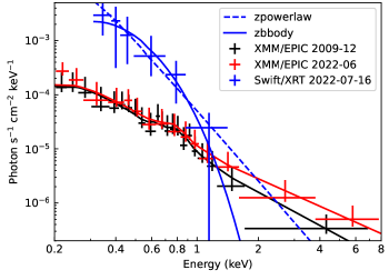
The X-ray emission of F01004-2237 shows intra-week variability in 2022, as seen from the XRT LC. Such a short time scale can be explained as the X-ray emission associated with the 2021 flare or a possible underlying AGN. To better distinguish between these two possibilities, we analyzed the X-ray spectra, including the new XMM-Newton/EPIC spectrum observed in 2022 (247 day) and the Swift/XRT spectrum during XF1 (281 day). We also analyzed the pre-flare spectrum taken by XMM-Newton/EPIC in 2009 for reference. We fit all the spectra with XSpec (version 12.13). All the errors reported in this subsection are at 90% confidence.
Nardini & Risaliti (2011) had modeled the 2009 spectrum by the sum of a MEKAL component and a powerlaw component. We fit the spectrum with the same data (black in Fig. 11), yielding a temperature of keV for the MEKAL component and an index of for the power-law component, which is consistent with the values of Nardini & Risaliti (2011) within the margin of error. The parameters suggest a starburst origin for the X-ray emission in 2009. The EPIC count rate in the 2022 observation increased by 3.4, or by a factor of , compared with that in the 2009 observation. This suggests an additional X-ray emission component in 2022. To investigate the spectral shape of the additional component, we fit the 2022 spectrum with a model containing three components: the first two are the same as those that fit the 2009 spectrum with fixed parameters, while the third is an additional power-law with free parameters. The model fits the data well with of (red in Fig. 11). The additional component has a power-law index of , implying that it is rather hard.
The spectrum of the XF1 on 281 day is rather soft, and only photons below 1.5 keV were detected. A powerlaw model with and a blackbody model with eV can both fit the spectrum with values of 0.6 and 0.7, respectively, for .
3.5.3 Origin of the X-ray emission
The additional component in the 2022 XMM-Newton spectrum is flat with a power-law index of . Such a flat spectrum is unlikely to be produced by a TDE because TDEs typically show soft and steep spectra (Saxton et al. 2020). Although some TDEs have flat and hard power-law components in their X-ray spectra (e.g., ASASSN-15oi, Holoien et al. 2016a), these components are much weaker than the soft thermal components and do not conform to the observation of F01004-2237. A possible underlying AGN can explain the flat spectrum because the spectral index roughly agrees with the typical AGN values of (Piconcelli et al. 2005) within the margin of error. The 2–10 keV luminosities in the 2009 and 2022 spectra are and erg s-1, respectively. Considering the starburst contribution in 2009, the AGN X-ray luminosity has changed by a factor of 4, which is typical for long-term X-ray variability of AGNs. Thus, the difference between the two XMM-Newton spectra can be interpreted as a long-term variation of AGN. We will discuss in Section 4.1 whether such an AGN exists based on multi-band data.
We also considered the possibility that the additional component could be related to the 2010 flare. Because the 2010 flare caused a [Fe VII] and [Fe X] coronal emission line echo (Tadhunter et al. 2017, 2021), it must be X-ray bright, although there are no direct X-ray observations to prove this. The X-ray emission of the 2010 flare should have faded over 12 years, and possible late-time emission should be soft and cannot explain the observed flat spectrum. However, it is also possible that the X-ray peak luminosity of the 2010 flare was Compton scattered by surrounding gas and caused a Compton echo, as was proposed to explain the diffused X-ray emission in the galactic centre (Koyama et al. 1996; Yu et al. 2011) and the X-ray afterglow of Swift J1644+57 (Cheng et al. 2016). Compton echoes are expected to have relatively flat spectra, consistent with the observations. A large amount of ionized gas at pc-scale is required to produce an echo lasting for a decade. This condition is satisfied in F01004-2237 because the coronal emission line echo lasts for at least 8 years (Tadhunter et al. 2021). Thus, we inferred that the additional component in June 2022 has two possible origins: the long-term variability of an AGN with X-ray luminosity of several erg s-1, or a Compton echo from the X-ray bright 2010 flare.
The X-ray flares discovered from the XRT LC on around 280 and 350 days have variability time scales of no more than 2–3 weeks and, therefore, must come from the vicinity of the SMBH. Its spectrum is too steep (powerlaw index ) to be emission of an AGN. Some galaxies have been reported to be AGNs with super-soft X-ray emissions, such as GSN 069 (Miniutti et al. 2013) and 2XMM J123103.2+110648 (Lin et al. 2013). However, they were later reclassified as TDEs (Shu et al. 2018; Lin et al. 2017) based on the long decay of their X-ray fluxes. Therefore, it is more likely that a TDE causes the X-ray flares. X-ray flares with less than 2–3 weeks time scales have been observed in other TDEs, such as AT 2019ehz and AT 2023lli (van Velzen et al. 2021; Huang et al. 2024). The flares were interpreted as a sudden decrease in the optical depth of the absorbing material enveloping the X-ray emitting region, possibly caused by the movement of discrete absorbing clouds. This interpretation may also apply to the 2021 flare of F01004-2237, during which the X-ray emission from the nuclear region is obscured by the envelope for most of the time, and is exposed only during the two X-ray flares.
3.6 Radio observations

Prior to its 2021 flare, F01004-2237 was observed and detected by VLA at 1.4, 5.5, 9.0, and 14.0 GHz between 2015 Oct and 2016 Aug (Hayashi et al. 2021). As shown in Fig. 12, the radio SED can be fitted with a synthrotron emission model using an MCMC fitting technique (e.g., Goodwin et al. 2022; Zhang et al. 2024). In order to probe whether the radio emission is enhanced following the 2021 flare of F01004-2237, i.e., a nascent jet or outflow was launched, we proposed high frequency (Ku- and K-band) observations with VLA (Program ID 22A-507; PI, Shu) on 2022 July 21. The data were reduced following standard procedures with the CASA package (CASA Team et al. 2022), and the source is clearly detected at both bands. We used the IMFIT task in CASA to fit the radio emission component with a two-dimensional elliptical Gaussian model to determine the position, and the integrated and peak flux density. A comparison of the integrated flux to the peak flux density indicates that the radio emission is compact, and no extended component is detected. By plotting the integrated flux density in Fig. 12, we found no excess in the radio emission in comparison with the flux densities extrapolated from the best-fit synthrotron emission model. Therefore, there is no obvious radio brightening since the 2021 optical flare, at least at the time of our VLA radio observations.
IRAS F01004-2237 was also observed by the Very Long Baseline Array (VLBA) on 2022 May 6 (Hayashi et al. 2024) although the observation was not designed to study this flare. A compact source was detected at 8.4 GHz on a 1 pc scale. Its position is consistent with the galaxy center measured by Gaia with an offset of only 3 mas, and its peak flux is 0.6 mJy beam-1. The compact source could be related to the long-standing AGN, or it could be related to the optical flare. With the available data, we cannot distinguish between these two possibilities. New high-resolution radio observations in the future may detect changes in the flux or position of this compact source, thereby solving the mystery of its origin.
4 The nature of the 2021 flare
In this section, we discuss the nature of the 2021 flare. We have ruled out a possibility of SLSNe with a nearly constant photospheric temperature of 22000 K from 99 to 219 day and VBELs with H FWHMs up to 17,000–19,000 km s-1 from 95 to 325 day. We therefore considered two possible origins associated with SMBH accretion, including TDE and AGN flare.
4.1 Constrains on pre-flare nuclear activity
We checked the level of possible nuclear activity before the flare occurred. This is not easy, as F01004-2237 shows vigorous starburst activity, which could overwhelm possible AGN signals. To make matters worse, there are Wolf-Rayet (WR) stars in the nucleus (Armus et al. 1988; Farrah et al. 2005; Tadhunter et al. 2017), producing some features similar to AGNs.
No broad emission lines (BELs) were detected in any of the optical spectra before the 2010 flare, including CTIO spectrum in 1985 (Armus et al. 1988), KPNO spectrum in 1995 (Veilleux et al. 1999; Lípari et al. 2003), HST/STIS spectrum in 2000 (Farrah et al. 2005), and WHT spectrum in 2005 (Rodríguez Zaurín et al. 2013). There is neither Pa BEL in the NIR spectrum taken in 1995 (Veilleux et al. 1997). The non-detection of BELs, even in the NIR band, cannot be explained by the obscuration of extremely thick dust. This is because the vicinity of the SMBH must be seen directly as VBELs with FWHMs km s-1 were detected after the 2021 flare, with fluxes varying within months, and the ratio of Ly/H indicates little dust reddening. Therefore, the non-detection of BELs is because they are intrinsically weak.
In addition, the X-ray spectra before the 2010 flare can be explained by starburst alone, without needing a power-law AGN component (Teng & Veilleux 2010; Nardini & Risaliti 2011). This cannot be explained by a Compton thick AGN, as proposed by (Nardini & Risaliti 2011), because X-ray emission with a steep spectrum varying in weeks was detected after the 2021 flare, indicating little gas absorption in the line of sight. Thus, we concluded that the nuclear activity must be weak before the 2010 flare. We had measured a 2–10 keV luminosity of erg s-1 using the 2009 spectrum, consistent with that measured by Nardini & Risaliti (2011). We adopted this luminosity as the upper limit of X-ray luminosity of AGN in 2009 and estimated an upper limit of bolometric luminosity of erg s-1 using a correction factor of 12 from Hopkins et al. (2007).
4.2 TDE versus AGN flare
We discuss the two possible interpretations of the 2021 flare in terms of shapes of LC, UV/optical SED and luminosities, parameters of VBELs, and X-ray to UV/optical luminosity ratios.
TDEs typically have smooth LCs rising quickly and falling slowly, in line with the observation of the 2021 flare, which rose in 50 days and dropped by 2–3 magnitudes in one year. However, the LCs of AGN flares, taking observations of changing-look AGNs as examples (e.g., Ricci & Trakhtenbrot 2023), showed rich diversity without a uniform pattern. Some AGN flares have LCs resembling those of TDEs, such as AT 2018dyk (Frederick et al. 2019). Thus, the LCs support a TDE interpretation but do not exclude the possibility of AGN flare.
The UV/optical SEDs of the 2021 flare can be well described by blackbody curves with temperatures 22,000 K, consistent with optical TDEs (e.g., van Velzen et al. 2021; Hammerstein et al. 2023). Meanwhile, the UV-optical SEDs of AGNs are generally close to power-law curves. However, it is challenging to distinguish a blackbody with a temperature of 22,000 K and a slightly extinct power-law, as they have little difference in observable wavelength ranges. We tried to model the observed SEDs from Swift/UVOT with power-law curves, yielding similarly good fits as blackbody curves with no statistically significant differences. We did not make a similar distinction using spectral data considering the interference from observed VBELs, possible other VBELs from He and metal elements, and possible Balmer continuum and Fe II emission. If assuming a SED similar to AGNs, we estimated a peak bolometric luminosity of erg s-1 using the measured peak at 4400 Å of erg s-1 and adopting a bolometric correction of 10 from Hopkins et al. (2007). We had demonstrated in section 4.1 that the pre-flare nuclear activity, if present, had a bolometric luminosity of erg s-1. Then, the variation has an amplitude of more than two orders of magnitude, which is rare among AGN flares. Thus, the UV/optical SED and luminosities support the TDE interpretation but do not exclude AGN flare.

The 2021 flare shows VBELs in H, H, He II 4686, He I 5876 and Ly between 105 and 325 days. The FWHM of H can reach 16,000–19,000 km s-1, and that of He II can even reach 21,000 km s-1, although the latter relies on the decomposition of He II with H. VBELs and strong He II emission distinguish TDEs from AGNs (Zabludoff et al. 2021). As can be seen from Fig. 13, the H FWHMs and He II/H ratios in F01004-2237 are consistent with those of TDEs (Charalampopoulos et al. 2022). To understand the properties of BELs in AGNs, we selected 3119 SDSS DR7 quasars with a signal-to-noise ratio of H BEL 10 using measurements by Shen et al. (2011). Among them, 99.87% have H FWHM 16,000 km s-1. Shen et al. (2011) did not measure the fluxes of He II, nor could we find any other literature that systematically investigated the He II fluxes in AGNs. This is not surprising, as in most quasars and Seyfert 1 galaxies, He II BELs can not be detected because they are weak and overwhelmed in the Fe II bump. Vanden Berk et al. (2001) measured the He II and H fluxes in the composite spectrum of SDSS quasars. With their measurements, we estimated an average He II/H ratio in quasars of 0.0045, much smaller than in F01004-2237. We found four SDSS DR7 quasars (0.13%) with H with FWHM 16,000 km s-1, and show their spectra in Fig. 14. One of them is a well-studied quasar 3C 332. It shows BELs with clear double-peak structures, which are thought to be emission from an accretion disk viewed from an inclined line of sight (Halpern 1990). Of the other three, J1027+6050 and J1605+2309 also show H with a double-peak structure, and J1334-0138 has an H emission line profile that deviates from a single Gaussian. None of the four show clear He II BELs, as their weak emission features around 5000 Å can be explained by H. All of these are inconsistent with VBELs in F01004-2237. Therefore, the properties of VBELs strongly favour the TDE interpretation other than the AGN flare interpretation.

Most of the time after the 2021 flare, the X-ray emission is weak. During two X-ray flares around 280 and 350 day, there are significant enhancements in X-ray emission lasting no more than weeks. On one hand, weak and highly variable X-ray emission is consistent with TDEs. Only 4 out of 17 ZTF TDEs in the sample of van Velzen et al. (2021) show clear X-ray detection. Their optical-to-X-ray ratios, expressed as ratios between UV/optical blackbody luminosity and 0.3–10 keV X-ray luminosity, are between 1 and 2000. The same ratio during XF1 in F01004-2237 is 2–6, which is calculated assuming a power-law or a blackbody X-ray spectrum, and is consistent with X-ray bright TDEs. On the other hand, X-ray emission is prevalent in AGNs. The relative strength of X-ray emission in AGNs is described using , calculated with the fluxes at 2 keV and 2500 Å (Tananbaum et al. 1979). We computed of the 2021 flare using XMM-Newton data on 247 day and Swift/XRT data on 281 day, and list the results in Table 4. The former was considered to be a lower limit because the X-ray emission on 247 day does not necessarily come from the 2021 flare. The latter was calculated assuming a power-law or a blackbody X-ray spectrum, respectively. Using the correlation between and in AGNs (Lusso et al. 2010), the predicted is only . The observed values are larger than the predicted values after considering the scatter of the correlation of 0.15, indicating that the X-ray emission is weaker relative to the UV emission during the 2021 flare than in AGNs. Therefore, the X-ray to UV/optical luminosity ratios favor the TDE interpretations.
| phase | measured | Log | predicted |
|---|---|---|---|
| (day) | (erg s-1 Hz-1) | ||
| 247.4 | 28.76 | 1.25 | |
| 281.5 | (pl) | 28.41 | 1.20 |
| (bb) |
- •
In summary, we concluded that the 2021 flare is a TDE.
5 The nature of the recurring flares
Table 5 lists the basic properties of the two flares in F01004-2237. The peak luminosity and energy budget of the 2010 flare were collected from Tadhunter et al. (2017) and Dou et al. (2017), which were estimated using V-band data and MIR data, respectively. Taking the intersection of the results from the two works, we obtained a peak luminosity of erg s-1 and a total energy of erg, which are both higher than those of the 2021 flare. The time interval of the peaks of the two flares is yr in the rest frame. In this section, we discuss the possible origins of the flare’s recurrence under the premise that the 2021 flare is TDE.
| 2010 flare | 2021 flare | |
| (MJD) | ||
| ( erg s-1) | 0.4–14 (T17) | |
| 4–11 (D17) | ||
| ( erg) | 0.3–11 (T17) | |
| 1–2 (D17) |
- •
5.1 The nature of the 2010 flare
As mentioned in the introduction section, Tadhunter et al. (2017) considered the 2010 flare as a TDE other than an AGN flare because of the He II BEL with large He II/H ratio in the spectrum 5 years after the flare occurred. In recent years, a new class of BF AGN flares has been identified, and examples are AT 2017bgt, OGLE17aaj, AT 2021loi, and AT 2019aalc (Trakhtenbrot et al. 2019; Gromadzki et al. 2019; Makrygianni et al. 2023; Milán Veres et al. 2024). These flares are characterized by a strong N III 4640 BF emission line with similar intensity to He II 4686, both commonly seen in TDEs. Trakhtenbrot et al. (2019) and subsequent works demonstrated that these flares are not TDEs because their emission lines are narrower than typical TDEs and their LCs show double-peak structures, and suggested that they originate from a sudden enhancement of the long-existing accretion flow. They also placed the 2010 flare in F01004-2237 into this class as they claimed similarity between the spectra of F01004-2237 and BF AGN flares.
However, the claimed similarity is questionable because there are two crucial differences that need to be explained131313We caution readers that it may be misleading to compare the 2015 spectrum directly to those of BF flares without removing the long-standing WR features and NELs from the host galaxy as some works did.. One is that the BELs in F01004-2237 are broader and show a significant change in width. The FWHMs of BELs are 6,000 km s-1 in the 2015 spectrum (Tadhunter et al. 2017), and can reach 16,000–19,000 km s-1 after the 2021 flare. For comparison, the BEL widths of the BF flares are between 2,000 and 5,000 km s-1 and do not change dramatically over time. The other is that He II in F01004-2237 is stronger relative to H. In the 2015 spectrum, the He II/H ratio is if emission from all sources are included, and is if contributions from WR stars and ISM are removed (Tadhunter et al. 2017). For comparison, the BF flares show He II/H ratios of 0.4–0.7. The large and variable width and the large He II/H ratio of BELs are prevalent in TDEs, and BF lines are more common in TDEs than in AGNs (e.g. van Velzen et al. 2020). Thus, we considered that the 2010 flare in F01004-2237 is more similar to TDEs than AGN flares.
We re-examined the nature of the 2010 flare in light of new observations of the 2021 flare. If the 2010 flare were indeed an AGN flare as proposed by Trakhtenbrot et al. (2019), the He II emission lines in the 2015 spectrum would indicate a broad line region with bulk velocities of several km s-1. The broad line region would still exist after the 2021 flare as the dynamic time scale is typically yr, and would produce an emission component with a similar width as in 2015. In fact, no such component in He II or other emission lines has been detected in early-time spectra taken after the 2021 flare. The difference in the ionization continuum can hardly explain the no detection because the 5100 Å luminosities at the time when these spectra were taken are erg s-1, similar to that in 2015. Thus, the new observations do not support the AGN flare interpretation, and we preferred that a TDE causes the 2010 flare. Note that the questions raised by Trakhtenbrot et al. (2019) about the TDE interpretation have been answered by Tadhunter et al. (2021) and Cannizzaro et al. (2021).
5.2 Repeating partial TDEs?
If related, the recurring flares in F01004 may be caused by repeating partial TDEs or double TDEs.
After a partial TDE occurs, the stellar remnant may return, producing the next TDE. The partial TDE of a star intruding in a parabolic orbit could transfer the stellar remnant into an elliptical orbit due to the weak asymmetry of the disrupted material. However, the period would be yr (Ryu et al. 2020), which cannot explain the 10.3 yr interval between the two flares. Therefore, repeating TDEs with an interval of 10.3 yr requires that the star was already in an elliptical orbit around the SMBH with a period of years before the disruption.
The observed period corresponds to an orbital semi-major axis AU for an SMBH mass of . For a partial TDE to occur, the pericenter must be similar to , which is AU for sun-like stars. Then, the orbit must be highly eccentric with . Such an orbit can be explained by the Hills mechanism. If so, the orbital semi-major axis of the captured star is related to the initial orbital parameters of close binary stars (Pfahl 2005) as:
| (8) |
where and are the binary semi-major axis and total mass, and is the mass of the ejected star. Assuming both the binary stars have a mass of 1 , the observed period corresponds to . The inferred binary semi-major axis is reasonable as it is far enough to avoid a common envelope, and close enough to avoid disintegration in collisions with fellow stars (Hills 1988).
Simulations show that the flare produced by a partial TDE has a steeper descent in the late-time, obeying rather than as in full TDEs (e.g., Coughlin & Nixon 2019; Miles et al. 2020). We tested this with the observations of the 2021 flare in F01004-2237. We fit the ATLAS/o, ATLAS/c and Swift UVW2 LCs after 60 day with t-9/4 curves. The procedure was similar to the fitting with t-5/3 curves (Section 3.2), except that we replaced the powerlaw index in the equation (3) with . This slightly improves the fit as the /d.o.f. decreases from 3.57 to 3.31, with d.o.f.. Therefore, t-9/4 curves agree slightly better with the data than t-5/3 curves, which supports the partial TDE model.
5.3 Double TDEs of binary stars?
There is a rich diversity of possible outcomes for the binary-SMBH encounter, with one possibility being that both stars are tidally disrupted (Mandel & Levin 2015; Mainetti et al. 2016). This phenomenon, known as double TDE, occurs when the pericenter of the binary’s centre of mass is close enough to the black hole. However, the time interval between the two TDEs is generally less than days, resulting in only one flare being observed, which is inconsistent with the situation in F01004-2237.
In the double TDE regime, two possible scenarios could explain the interval of 10.3 yr. One scenario was proposed by Mandel & Levin (2015) to interpret the two flares 20 years apart in IC 3599. A possible outcome of the binary-SMBH encounter is that one star is directly disrupted, causing the first TDE, and then the other star is captured into an elliptical orbit and produces the second TDE when it returns to the pericenter. According to the simulations of Mandel & Levin (2015), the orbital period of the captured star can range from 6 months to several decades, explaining the observations in F01004-2237.
The other scenario involves the encounter between a stellar binary and a mpc-scale SMBHB binary. As shown in the simulations by Wu & Yuan (2018) and Coughlin et al. (2018), there is a significant probability of delayed double TDEs, among which the time interval of two TDEs can be more than ten years. A mpc-scale secondary SMBH may pass through the stellar debris stream of the TDE as it orbits the primary SMBH and cause periodic gaps on the X-ray LC (Liu et al. 2014; Shu et al. 2020). Unfortunately, the X-ray emission from the flare in F01004-2237 is weak and cannot be used to test the presence of mpc-scale secondary SMBH.
5.4 Two independent flares?
We considered the possibility that the two flares are not associated physically. The probability of a TDE (the 2021 flare) occurring in a time interval after a specific event (the 2010 flare) is , where is the incidence rate of TDE per galaxy in a unit of yr-1. Adopting the rate of optical TDEs of yr-1 (Yao et al. 2023) and yr, we estimated a small probability of .
For to increase to , the TDE rate needs to be yr-1, times higher than in normal galaxies. Thus, assuming the two flares are independent requires an extremely high TDE rate in F01004-2237. On the contrary, assuming that the two flares are repeating partial TDEs or double TDEs does not require such a high TDE rate because they should be treated as “a single event” when calculating the probability.
As there are many theories to explain the high TDE rate in post-starburst galaxies, we examined if they also apply to F01004-2237. First, a starburst can cause an unusually high concentration of stars in the nucleus, enhancing the TDE rate (Stone & Metzger 2016; Stone & van Velzen 2016). In theory, this effect subsides over time (Stone et al. 2018). The starburst in F01004-2237 started only 3–6 Myr ago, as estimated by the age of the WR stars (Tadhunter et al. 2017). Based on the results of Stone et al. (2018), we inferred that the TDE rate in F01004-2237 may be 1–2 orders of magnitude higher than that in post-starburst galaxies with stellar ages of 100 Myr, and hence 2–3 orders of magnitude higher than in normal galaxies.
Second, a nuclear star cluster (NSC) can enhance the TDE rate by orders of magnitude in galaxies with different masses and various types (Pfister et al. 2020). The HST images show a point-like source in the nucleus of F01004-2237, with SED consistent with a young stellar population with an age of Myr and a mass of (Surace et al. 1998). The source is barely resolved, indicating a pc size. This supports the existence of an NSC in F01004-2237, with mass and age unusual among NSCs in galaxies. How much such an NSC can raise the TDE rate remains to be answered by theoretical studies.
Third, the presence of a companion SMBH with a mass ratio of 0.01–0.1 can significantly boost the TDE rate (e.g., Ivanov et al. 2005). According to the simulations (e.g., Chen et al. 2009; Li et al. 2017), in a phase lasting for Myr, during which the SMBHs are pc apart, the TDE rate could be as high as yr-1. Although there is no direct evidence, F01004-2237 may also host a pc-scale SMBH binary, given that starbursts are generally associated with mergers, which can lead to SMBH binaries. There are no obvious merger signals in the HST image (Surace et al. 1998). However, this cannot negate the scenario of SMBH binary, because non-equal mass SMBH binaries may be related to minor mergers, and fall to the pc-scale long after mergers.
Therefore, a high TDE rate of yr-1 in F01004-2237 is possible in theory. As a result, we cannot rule out the possibility that the two flares are independent.
6 Discussions
6.1 Evidence of pre-flare AGN claimed by literatures
Some literature claimed to have found evidence for luminous AGN based on Seyfert-like optical narrow emission line (NELs) ratios (e.g., Allen et al. 1991; Yuan et al. 2010). We noticed that the classification based on narrow emission lines is controversial in the literature, as Veilleux et al. (1999) classified it as star-forming. The optical NELs show a narrow component with FWHM of 90 km s-1 and broad components blueshifted by km s-1, which is considered to be related with outflow (Lípari et al. 2003; Rodríguez Zaurín et al. 2013; Tadhunter et al. 2021). Rodríguez Zaurín et al. (2013) shows that while the narrow component has starforming-like line ratios, the broadest component has Seyfert-like line ratios. This may be why previous literature made contradictory classifications, as pointed out by Tadhunter et al. (2017). The outflow component that shows Seyfert-like line ratios has a radial extent to 3.5 kpc, as measured by Rodríguez Zaurín et al. (2013) using long-slit spectroscopy. Meanwhile, it is not detected in the STIS 2000 spectrum extracted within an aperture corresponding to 350 pc in physical (Farrah et al. 2005). Thus, its distance to the centre is pc and thus traces AGN activity years ago. However, the levels of nuclear activity may vary dramatically on such a time scale, an example being Arp 187 (Ichikawa et al. 2019). We are more concerned about recent activity, for which NELs in the nuclear spectrum are needed for diagnosis. As measured by Farrah et al. (2005), the NEL line ratios in the nuclear region fall around the classification lines between AGN and starforming (Kewley et al. 2001, 2006), and classifications based on [S II]/H and [O I]/H are different. Note that the result depends on the choice of classification lines; for example, the line ratios will be the explicit starforming type if the classification lines of Veilleux & Osterbrock (1987) are used. The classification lines of Kewley et al. were calculated assuming the Salpeter’s initial mass function, while the presence of a large population of WR stars in the nuclear region of F01004-2237 may result in line ratios closer to Seyfert galaxies than in normal star-forming galaxies. Thus, spectral analysis in the nuclear region does not show evidence of strong AGN in recent years. This is consistent with the absence of BELs and the weak hard X-ray emission.
The MIR spectrum of F01004-2237 shows only week PAH emission features with equivalent widths lower than expected for starburst galaxies (Tran et al. 2001; Imanishi et al. 2007; Veilleux et al. 2009). This was considered to be evidence of AGN, whose intense X-ray and EUV emissions can destroy PAHs (e.g., Voit 1992). However, a weak AGN at present and a strong AGN in the past can also explain the destruction of PAH, and a strong AGN at present is not necessary.
F01004-2237 shows a hotter IR SED than starforming galaxies. The IR SED indexes, such as flux ratios between 30 and 15 m, and between MIR to FIR, are all consistent with ULIRGs with clear AGNs (Veilleux et al. 2009). However, the MIR continuum of F01004-2237 shows only a weak 9.7 m silicate absorption feature, and does not show strong dust temperature gradients (Imanishi et al. 2007; Veilleux et al. 2009), both of which are expected to be signatures of a buried AGN. This leads us to suspect that the warm dust radiating the MIR continuum may have illumination sources other than the AGN. As previously mentioned, F01004-2237 hosts an NSC with an age of Myr, a mass of , and a size of pc. Such an NSC may create a dense radiation field, producing a higher dust temperature than normal star-forming galaxies. Moreover, considering that two energetic flares occurred in recent 14 years in F01004-2237, other flares possibly occurred in decades prior to the Spitzer observations in 2004, although no observations were available to test them. The 2010 flare was accompanied by a bright dust echo lasting for at least ten years, resulting in increases of monochromatic luminosities at 3.4 and 4.6 m of erg s-1 (Dou et al. 2017). If the hypothetic earlier flares also had similar total energies, they might significantly increase the temperature of the nuclear dust, producing an IR SED mimicking those of AGNs. Therefore, it is not reliable to estimate the level of AGN with MIR luminosity.
6.2 Comparison with known recurring flares
| ID | z | log | / | / | Ref. | |||||
| (1) | (2) | (3) | (4) | (5) | (6) | (7) | (8) | (9) | (10) | (11) |
| ASASSN-14ko | 0.0425 | 7.9 | 21 | 0.31 | * | - | 1,2,3 | |||
| eRASSt J0456 | 0.077 | 7.0 | 5 | 0.6 | 0.4 | - | 4,5 | |||
| AT 2022dbl | 0.0284 | 6.4 | 2 | 1.89 | * | 0.4 | 2026/01 | 6 | ||
| AT 2020vdq | 0.045 | 6.1 | 2 | 2.54 | 30 | 2026/01 | 7 | |||
| AT 2018fyk | 0.059 | 7.7 | 2 | 3.1 | 0.02 | 2025/03 | 8,9 | |||
| F01004-2237 | 0.1178 | 7.4 | 2 | 10.3 | 0.05–0.5 | 2033 | 10,11 | |||
| IC 3599 | 0.0215 | 6.7 | 2 | 18.8 | * | 0.3? | 2029 | 12,13,14 | ||
| RX J1331-3243 | 0.0519 | 6.5 | 2 | 27.5 | - | 0.6? | 2050 | 15,16 | ||
-
•
(1): The identification of the flares (eRASSt J045650.3-203750 and RX J133157.6-324319.7 are listed as short names). (2): Redshift. (3): Black hole mass in a unit of . For IC 3599, we adopted value from Grupe et al. (2015). (4): Number of flares reported. Note that we did not adopt the three-flares model for IC 3599 proposed by Campana et al. (2015) because the predicted flare in 2019 was not seen (Grupe et al. 2024). (5): The time interval of the observed peaks of the flares in a unit of years in the rest frame. (6)(7): The total energies (if present in the literature) and the peak luminosities of the first and the second flares. We list the energies and luminosities in 0.2–2 keV for those flares detected in the X-ray band, and the values in the UV band from blackbody fit for other flares. For ASASSN-14ko, all flares have similar luminosities, so we list the average for the flares studied in detail. For IC 3599 and RX J1331-3243 with sparse data sampling, we adopted the observed peak luminosities as lower limits. (8): The total energy of the most energetic flare. The values with a “*” label are our own estimates based on literature data, which is not accurate and only used for order of magnitude estimates. Others are taken directly from the literature. The total energy of flares in RX J1331-3243 cannot be estimated due to a lack of observational data. (9): The ratio between the energies of the second and the first flares. If energies are absent in the literature, we calculated the ratio between peak luminosities. Note that the ratios are only for reference for IC 3599 and RX J1331-3243 with only lower limits of luminosities. (10): The predicted peak time of the next flare for those occurring only twice. (11): References are: 1. Payne et al. (2021); 2. Payne et al. (2022); 3. Payne et al. (2023); 4. Liu et al. (2023b); 5. Liu et al. (2024); 6. Lin et al. (2024); 7. Somalwar et al. (2023); 8. Wevers et al. (2019); 9. Wevers et al. (2023); 10. Tadhunter et al. (2017); 11. Dou et al. (2017); 12. Grupe et al. (1995); 13. Grupe et al. (2015); 14. Campana et al. (2015); 15. Hampel et al. (2022); 16. Malyali et al. (2023).
In this section, we compared the recurring flares in F01004-2237 and other galaxies. We check whether all of them can be interpreted under the framework of repeating partial TDEs, as this is how most of the literature explains them. The information on these flares is listed in Table 6. X-ray QPEs are not listed here because their time scales, luminosities and energy budgets are quite different from flares in F01004-2237.
In the scenario of repeating partial TDEs formed by the Hills mechanism, the outcome of the captured star depends on parameter . The star is partially disrupted if is greater than the critical value and is not disrupted otherwise. Depending on , repeating partial TDE can be divided into two groups. In one group, is only slightly above the critical value, causing only a tiny fraction of stellar mass to be disrupted, leaving flares with low energies and short durations (e.g., Ryu et al. 2020; Nixon et al. 2021). Since a partial TDE has little effect on and the stellar mass decreases only a little, is almost constant and similar partial TDEs can repeat many times. In the other group, is significantly larger than the critical value, causing a large fraction to be disrupted, resulting in energetic flares. Only several flares may be detected because the remaining flares are too weak due to small residual stellar mass.
This scenario can explain the diversity of the observational features of recurring flares. We divided all recurring flares into two groups based on the above analysis. The first group include ASASSN-14ko and X-ray QPEs, where flares were detected, and a single flare has a UV energy erg or an X-ray energy erg. The second group include the other recurring flares. We preferred that the difference in is decisive, while the other differences are not essential. The two groups appear to have different periods ( days for the first group and days for the second group). However, this might be a selection effect. Long-period, low-energy repeating partial TDEs might exist but be extremely difficult to identify. Short-period, energetic partial TDEs might also exist but be misclassified as a single TDE because the flares overlap. In addition, most flares in the first group were detected in the X-ray band, while flares in the second group could be detected in both the UV/optical and X-ray bands. The possible reason is that a larger debris mass leads to a higher chance of forming an optically thick envelop through debris collision or outflow, producing strong UV/optical emission (e.g., Dai et al. 2018).
In the scenario of repeating partial TDEs, will the debris mass of the next TDE be greater than, less than, or roughly equal to that of the previous one? It is challenging to give an exact answer because the remnant fraction has a complex relationship with the stellar mass and parameters, as shown in Fig. 4 of Ryu et al. (2020). To complicate matters further, stellar remnants that survive a partial TDE do not have enough time to reach equilibrium before returning (Ryu et al. 2020), and hence, when calculating the remnant fraction of the next TDE, the results of stars of the same mass cannot be simply reproduced. What is clear, however, is that the debris in the next TDE is unlikely to be much more massive than in the previous one. This is because if the stellar core survives a partial TDE as only (part of) the stellar envelope lost, its structure changes little before returning to the pericenter since the time scale of thermal relaxation is much longer than the orbital period (Ryu et al. 2020), and thus it is likely to survive the next partial TDE.
We tested this with observational data. Most recurring flares meet theoretical expectations as the next flare is weaker than or similar to the previous one in total energy and peak luminosity. The only exception is AT 2020vdq, where the second flare is 15 times brighter than the first and has total energy 30 times higher (Somalwar et al. 2023). This is difficult to understand in the scenario of repeating partial TDEs. Meanwhile, in the double TDEs scenario, two flares are produced by two different stars in the binary system, and there is no direct correlation between their luminosities and energies. In addition, only two flares have been detected so far for AT 2020vdq, not contradicting a double TDEs scenario. Thus, AT 2020vdq may be a case of double TDEs, rather than repeating partial TDEs.
If AT 2020vdq is double TDEs, then the other recurring flares appearing only twice may also be double TDEs, because situations where the second flare is stronger than, weaker than or similar to the first one can all occur in the double TDEs scenario. However, it is more likely that ASASSN-14ko and eRASSt J045650.3-203750 are repeating partial TDEs because they show multiple flares. Therefore, we proposed that the recurring flares detected so far could not be explained with only one scenario, and repeating partial TDEs and double TDEs may both exist.
6.3 Future predictions
For sources that have flared only twice currently, the best way to distinguish between the repeating partial TDEs and the double TDEs scenarios is to wait and check if there is an expected third flare. We list the timing of these expected flares in the repeating partial TDEs scenario in Table 6. The next flare expected in F01004-2237 will peak between December 2032 and August 2033. However, it may come earlier, considering that the flare interval in eRASSt J045650.3-203750 is gradually shortening (Liu et al. 2024). A flare that arrives at the scheduled time and is weaker than the previous one supports an interpretation of repeating partial TDEs, while the nondetection of the expected flare supports interpretations of double TDEs or independent TDEs. Before that, AT 2018fyk, AT 2020vdq and AT 2022dbl will go to trials in 2025 and 2026.
In section 5.4, we demonstrated that a high TDE rate of in F01004-2237 is required if the two flares are independent. Theoretically, a galaxy with a young starburst and massive NSC, like F01004-2237, may have a high TDE rate. This can be tested by future monitoring of a large number of WR galaxies (e.g., Brinchmann et al. 2008) with similar properties. With the advent of new generation sky surveys such as the 2.5-meter Wide Field Survey Telescope (Wang et al. 2023) and the Large Synoptic Survey Telescope (Ivezić et al. 2019), TDEs with magnitudes can be detected, meaning that the monitoring we mentioned earlier can be performed in . Within this large volume, there are at least a few hundred galaxies with properties similar to F01004-2237, taking into account the cosmological evolution of the star formation rate. Monitoring them over several years is sufficient to prove or disprove the possible high TDE rate.
7 Summary and conclusions
A decade after the flare in 2010, a second optical flare was discovered on September 4, 2021, by ATLAS with in F01004-2237. The flare was later independently detected by Gaia, which showed that the flare’s position coincides with the galaxy centre. The flare peaks in days with , , and , corresponding to absolute magnitudes of . After the peak, the flare drops roughly as and falls below the detection limit in all bands after 700 day. Between 99 and 219 day, the flare maintains a nearly constant blackbody temperature of 22,000 K despite declining luminosity. All these features are consistent with TDEs and inconsistent with SNe. The multi-band LCs can be well fit by a TDE model, yielding a peak luminosity of erg s-1, and a total energy of erg released in 700 days.
The optical and UV spectra of the flare taken between 95 and 325 day show VBELs with FWHM km s-1, detected in H, H, He II 4686, He I 5876 and Ly. H and He II VBELs have been continuously observed over more than 200 days, with H FWHM varying from 7,000 to 19,000 km s-1 and He II FWHM reaching km s-1, and He II/H ratios ranging from 0.3 to 2.3. Such VBELs must come from the vicinity of the SMBH, and a high Ly/H ratio of indicates little dust reddening in the line of sight. The large FWHMs and the high He II/H ratios of the VBELs strongly support a TDE nature and can hardly be explained with SNe and AGN flares.
Most of the time after the 2021 flare, no X-ray emission clearly associated with the flare was detected. An XMM-Newton observation on 247 day shows that the X-ray emission is weak relative to the UV emission as , a value much higher than in AGNs with similar UV luminosity. Around 280 and 350 day, two X-ray flares were detected by Swift/XRT with confidences of 3.5 and 2.5, respectively. The flares last no more than 2–3 weeks, during which the X-ray spectrum is soft and can be described by a power-law with or a blackbody with eV with no additional absorption beyond the milky way. The soft, highly variable X-ray emission, which is weak relative to UV emission, supports a TDE nature.
Based on these observations, we conclude that a TDE caused the 2021 flare. In addition, as no BEL components with several km s-1 are seen in the new spectra, we prefer that the 2010 flare is also caused by a TDE. The time interval between the two flares is yr, and the energy released in the second flare is 0.05–0.5 times that in the first.
If physically related, the recurring flares in F01004-2237 could be explained by either repeating partial TDEs or double TDEs. We cannot distinguish between the two possibilities solely based on the observations of the two flares because theoretical works have yet to provide a straightforward means of distinguishing between them, at least until now. The repeating partial TDEs scenario predicts that the next flare will arrive in 2032 or 2033. Whether the flare occurs as scheduled can test the scenario.
If not physically related, the recurring flares require an extremely high TDE rate of . Such a rate is theoretically possible given that F01004-2237 has just experienced a starburst and that there is a young star cluster with an age of 3–6 Myr and a mass of , and could be tested by future photometric monitoring of galaxies with similar properties at .
Acknowledgements.
We acknowledge the anonymous referee for helping us improve this manuscript. We thank for useful suggestions from Fukun Liu and Takayuki Hayashi. We thank Minghao Yue for performing the Magellan observation. This work is supported by the National Natural Science Foundation of China (NFSC, 12103002). N.J. acknowledges the support of the NFSC (12073025, 12192221), the National Key R&D Program of China (2023YFA1608100), the Strategic Priority Research Program of the Chinese Academy of Sciences (XDB0550200). We thank the Swift science operations team for accepting our ToO requests and arranging the observations. This work made use of data supplied by the UK Swift Science Data Centre (UKSSDC) at the University of Leicester. Some of the observations reported in this paper were obtained with the Southern African Large Telescope (SALT), under program 2021-2-LSP-001 (PI: Buckley). Polish participation in SALT is funded by grant No. MEiN nr 2021/WK/01. Based on observations obtained at the international Gemini Observatory, a program of NSF NOIRLab, which is managed by the Association of Universities for Research in Astronomy (AURA) under a cooperative agreement with the U.S. National Science Foundation on behalf of the Gemini Observatory partnership: the U.S. National Science Foundation (United States), National Research Council (Canada), Agencia Nacional de Investigación y Desarrollo (Chile), Ministerio de Ciencia, Tecnología e Innovación (Argentina), Ministério da Ciência, Tecnologia, Inovações e Comunicações (Brazil), and Korea Astronomy and Space Science Institute (Republic of Korea). This research uses data obtained through the Telescope Access Program (TAP), which has been funded by the TAP member institutes. Observations obtained with the Hale Telescope at Palomar Observatory were obtained as part of an agreement between the National Astronomical Observatories, Chinese Academy of Sciences, and the California Institute of Technology.References
- Allen et al. (1991) Allen, D. A., Norris, R. P., Meadows, V. S., & Roche, P. F. 1991, MNRAS, 248, 528
- Arcodia et al. (2021) Arcodia, R., Merloni, A., Nandra, K., et al. 2021, Nature, 592, 704
- Armus et al. (1988) Armus, L., Heckman, T. M., & Miley, G. K. 1988, ApJ, 326, L45
- Bade et al. (1996) Bade, N., Komossa, S., & Dahlem, M. 1996, A&A, 309, L35
- Brinchmann et al. (2008) Brinchmann, J., Kunth, D., & Durret, F. 2008, A&A, 485, 657
- Bromley et al. (2012) Bromley, B. C., Kenyon, S. J., Geller, M. J., & Brown, W. R. 2012, ApJ, 749, L42
- Brown et al. (2016) Brown, P. J., Yang, Y., Cooke, J., et al. 2016, ApJ, 828, 3
- Brown et al. (2013) Brown, T. M., Baliber, N., Bianco, F. B., et al. 2013, PASP, 125, 1031
- Bruzual & Charlot (2003) Bruzual, G. & Charlot, S. 2003, MNRAS, 344, 1000
- Burgh et al. (2003) Burgh, E. B., Nordsieck, K. H., Kobulnicky, H. A., et al. 2003, in Society of Photo-Optical Instrumentation Engineers (SPIE) Conference Series, Vol. 4841, Instrument Design and Performance for Optical/Infrared Ground-based Telescopes, ed. M. Iye & A. F. M. Moorwood, 1463–1471
- Calzetti et al. (1994) Calzetti, D., Kinney, A. L., & Storchi-Bergmann, T. 1994, ApJ, 429, 582
- Campana et al. (2015) Campana, S., Mainetti, D., Colpi, M., et al. 2015, A&A, 581, A17
- Cannizzaro et al. (2021) Cannizzaro, G., Jonker, P. G., & Mata-Sánchez, D. 2021, ApJ, 909, 159
- CASA Team et al. (2022) CASA Team, Bean, B., Bhatnagar, S., et al. 2022, PASP, 134, 114501
- Charalampopoulos et al. (2022) Charalampopoulos, P., Leloudas, G., Malesani, D. B., et al. 2022, A&A, 659, A34
- Chen et al. (2022) Chen, J.-H., Dou, L.-M., & Shen, R.-F. 2022, ApJ, 928, 63
- Chen & Shen (2021) Chen, J.-H. & Shen, R.-F. 2021, ApJ, 914, 69
- Chen et al. (2009) Chen, X., Madau, P., Sesana, A., & Liu, F. K. 2009, ApJ, 697, L149
- Cheng et al. (2016) Cheng, K. S., Chernyshov, D. O., Dogiel, V. A., Kong, A. K. H., & Ko, C. M. 2016, ApJ, 816, L10
- Coughlin et al. (2018) Coughlin, E. R., Darbha, S., Kasen, D., & Quataert, E. 2018, ApJ, 863, L24
- Coughlin & Nixon (2019) Coughlin, E. R. & Nixon, C. J. 2019, ApJ, 883, L17
- Crawford et al. (2010) Crawford, S. M., Still, M., Schellart, P., et al. 2010, in Proc. SPIE, Vol. 7737, Observatory Operations: Strategies, Processes, and Systems III, 773725
- Cufari et al. (2022) Cufari, M., Coughlin, E. R., & Nixon, C. J. 2022, ApJ, 929, L20
- Dai et al. (2018) Dai, L., McKinney, J. C., Roth, N., Ramirez-Ruiz, E., & Miller, M. C. 2018, ApJ, 859, L20
- Davies et al. (1997) Davies, R. L., Allington-Smith, J. R., Bettess, P., et al. 1997, in Society of Photo-Optical Instrumentation Engineers (SPIE) Conference Series, Vol. 2871, Optical Telescopes of Today and Tomorrow, ed. A. L. Ardeberg, 1099–1106
- Dou et al. (2017) Dou, L., Wang, T., Yan, L., et al. 2017, ApJ, 841, L8
- Drake et al. (2011) Drake, A. J., Djorgovski, S. G., Mahabal, A., et al. 2011, ApJ, 735, 106
- Drake et al. (2009) Drake, A. J., Djorgovski, S. G., Mahabal, A., et al. 2009, ApJ, 696, 870
- Evans et al. (2009) Evans, P. A., Beardmore, A. P., Page, K. L., et al. 2009, MNRAS, 397, 1177
- Evans et al. (2007) Evans, P. A., Beardmore, A. P., Page, K. L., et al. 2007, A&A, 469, 379
- Evans et al. (2023) Evans, P. A., Nixon, C. J., Campana, S., et al. 2023, Nature Astronomy, 7, 1368
- Farrah et al. (2005) Farrah, D., Surace, J. A., Veilleux, S., Sanders, D. B., & Vacca, W. D. 2005, ApJ, 626, 70
- Frederick et al. (2019) Frederick, S., Gezari, S., Graham, M. J., et al. 2019, ApJ, 883, 31
- French et al. (2016) French, K. D., Arcavi, I., & Zabludoff, A. 2016, ApJ, 818, L21
- French et al. (2020) French, K. D., Wevers, T., Law-Smith, J., Graur, O., & Zabludoff, A. I. 2020, Space Sci. Rev., 216, 32
- Gaia Collaboration et al. (2018) Gaia Collaboration, Brown, A. G. A., Vallenari, A., et al. 2018, A&A, 616, A1
- Gal-Yam (2019) Gal-Yam, A. 2019, ARA&A, 57, 305
- Gezari et al. (2006) Gezari, S., Martin, D. C., Milliard, B., et al. 2006, ApJ, 653, L25
- Giustini et al. (2020) Giustini, M., Miniutti, G., & Saxton, R. D. 2020, A&A, 636, L2
- Goodwin et al. (2022) Goodwin, A. J., van Velzen, S., Miller-Jones, J. C. A., et al. 2022, MNRAS, 511, 5328
- Graur et al. (2018) Graur, O., French, K. D., Zahid, H. J., et al. 2018, ApJ, 853, 39
- Gromadzki et al. (2019) Gromadzki, M., Hamanowicz, A., Wyrzykowski, L., et al. 2019, A&A, 622, L2
- Grupe et al. (1995) Grupe, D., Beuermann, K., Mannheim, K., et al. 1995, A&A, 299, L5
- Grupe et al. (2015) Grupe, D., Komossa, S., & Saxton, R. 2015, ApJ, 803, L28
- Grupe et al. (2024) Grupe, D., Komossa, S., & Wolsing, S. 2024, ApJ, 969, 98
- Guillochon & Ramirez-Ruiz (2013) Guillochon, J. & Ramirez-Ruiz, E. 2013, ApJ, 767, 25
- Halpern (1990) Halpern, J. P. 1990, ApJ, 365, L51
- Hammerstein et al. (2023) Hammerstein, E., van Velzen, S., Gezari, S., et al. 2023, ApJ, 942, 9
- Hampel et al. (2022) Hampel, J., Komossa, S., Greiner, J., et al. 2022, Research in Astronomy and Astrophysics, 22, 055004
- Hayashi et al. (2021) Hayashi, T. J., Hagiwara, Y., & Imanishi, M. 2021, MNRAS, 504, 2675
- Hayashi et al. (2024) Hayashi, T. J., Hagiwara, Y., & Imanishi, M. 2024, ApJ, 970, 5
- Hills (1988) Hills, J. G. 1988, Nature, 331, 687
- Hodgkin et al. (2021) Hodgkin, S. T., Harrison, D. L., Breedt, E., et al. 2021, A&A, 652, A76
- Holoien et al. (2016a) Holoien, T. W. S., Kochanek, C. S., Prieto, J. L., et al. 2016a, MNRAS, 463, 3813
- Holoien et al. (2016b) Holoien, T. W. S., Kochanek, C. S., Prieto, J. L., et al. 2016b, MNRAS, 455, 2918
- Hopkins et al. (2007) Hopkins, P. F., Richards, G. T., & Hernquist, L. 2007, ApJ, 654, 731
- Hu et al. (2022) Hu, L., Wang, L., Chen, X., & Yang, J. 2022, ApJ, 936, 157
- Huang et al. (2024) Huang, S., Jiang, N., Zhu, J., et al. 2024, ApJ, 964, L22
- Ichikawa et al. (2019) Ichikawa, K., Ueda, J., Bae, H.-J., et al. 2019, ApJ, 870, 65
- Imanishi et al. (2007) Imanishi, M., Dudley, C. C., Maiolino, R., et al. 2007, ApJS, 171, 72
- Ivanov et al. (2005) Ivanov, P. B., Polnarev, A. G., & Saha, P. 2005, MNRAS, 358, 1361
- Ivezić et al. (2019) Ivezić, Ž., Kahn, S. M., Tyson, J. A., et al. 2019, ApJ, 873, 111
- Jiang et al. (2019) Jiang, N., Wang, T., Mou, G., et al. 2019, ApJ, 871, 15
- Kaiser et al. (2002) Kaiser, N., Aussel, H., Burke, B. E., et al. 2002, in Society of Photo-Optical Instrumentation Engineers (SPIE) Conference Series, Vol. 4836, Survey and Other Telescope Technologies and Discoveries, ed. J. A. Tyson & S. Wolff, 154–164
- Kankare et al. (2017) Kankare, E., Kotak, R., Mattila, S., et al. 2017, Nature Astronomy, 1, 865
- Kewley et al. (2001) Kewley, L. J., Dopita, M. A., Sutherland, R. S., Heisler, C. A., & Trevena, J. 2001, ApJ, 556, 121
- Kewley et al. (2006) Kewley, L. J., Groves, B., Kauffmann, G., & Heckman, T. 2006, MNRAS, 372, 961
- Kochanek et al. (2017) Kochanek, C. S., Shappee, B. J., Stanek, K. Z., et al. 2017, PASP, 129, 104502
- Könyves-Tóth & Vinkó (2021) Könyves-Tóth, R. & Vinkó, J. 2021, ApJ, 909, 24
- Koyama et al. (1996) Koyama, K., Maeda, Y., Sonobe, T., et al. 1996, PASJ, 48, 249
- Leloudas et al. (2016) Leloudas, G., Fraser, M., Stone, N. C., et al. 2016, Nature Astronomy, 1, 0002
- Li et al. (2017) Li, S., Liu, F. K., Berczik, P., & Spurzem, R. 2017, ApJ, 834, 195
- Lin et al. (2017) Lin, D., Godet, O., Ho, L. C., et al. 2017, MNRAS, 468, 783
- Lin et al. (2013) Lin, D., Irwin, J. A., Godet, O., Webb, N. A., & Barret, D. 2013, ApJ, 776, L10
- Lin et al. (2024) Lin, Z., Jiang, N., Wang, T., et al. 2024, ApJ, 971, L26
- Lípari et al. (2003) Lípari, S., Terlevich, R., Díaz, R. J., et al. 2003, MNRAS, 340, 289
- Liu et al. (2023a) Liu, C., Mockler, B., Ramirez-Ruiz, E., et al. 2023a, ApJ, 944, 184
- Liu et al. (2014) Liu, F. K., Li, S., & Komossa, S. 2014, ApJ, 786, 103
- Liu et al. (2022) Liu, X.-L., Dou, L.-M., Chen, J.-H., & Shen, R.-F. 2022, ApJ, 925, 67
- Liu et al. (2023b) Liu, Z., Malyali, A., Krumpe, M., et al. 2023b, A&A, 669, A75
- Liu et al. (2024) Liu, Z., Ryu, T., Goodwin, A. J., et al. 2024, arXiv e-prints, arXiv:2401.14091
- Lusso et al. (2010) Lusso, E., Comastri, A., Vignali, C., et al. 2010, A&A, 512, A34
- Mainetti et al. (2016) Mainetti, D., Lupi, A., Campana, S., & Colpi, M. 2016, MNRAS, 457, 2516
- Makrygianni et al. (2023) Makrygianni, L., Trakhtenbrot, B., Arcavi, I., et al. 2023, ApJ, 953, 32
- Malyali et al. (2023) Malyali, A., Liu, Z., Rau, A., et al. 2023, MNRAS, 520, 3549
- Malyali et al. (2021) Malyali, A., Rau, A., Merloni, A., et al. 2021, A&A, 647, A9
- Mandel & Levin (2015) Mandel, I. & Levin, Y. 2015, ApJ, 805, L4
- Martin et al. (2015) Martin, C. L., Dijkstra, M., Henry, A., et al. 2015, ApJ, 803, 6
- Mattila et al. (2018) Mattila, S., Pérez-Torres, M., Efstathiou, A., et al. 2018, Science, 361, 482
- Milán Veres et al. (2024) Milán Veres, P., Franckowiak, A., van Velzen, S., et al. 2024, arXiv e-prints, arXiv:2408.17419
- Miles et al. (2020) Miles, P. R., Coughlin, E. R., & Nixon, C. J. 2020, ApJ, 899, 36
- Miniutti et al. (2019) Miniutti, G., Saxton, R. D., Giustini, M., et al. 2019, Nature, 573, 381
- Miniutti et al. (2013) Miniutti, G., Saxton, R. D., Rodríguez-Pascual, P. M., et al. 2013, MNRAS, 433, 1764
- Nardini & Risaliti (2011) Nardini, E. & Risaliti, G. 2011, MNRAS, 415, 619
- Neustadt et al. (2020) Neustadt, J. M. M., Holoien, T. W. S., Kochanek, C. S., et al. 2020, MNRAS, 494, 2538
- Nixon et al. (2021) Nixon, C. J., Coughlin, E. R., & Miles, P. R. 2021, ApJ, 922, 168
- Oknyansky et al. (2019) Oknyansky, V. L., Winkler, H., Tsygankov, S. S., et al. 2019, MNRAS, 483, 558
- Payne et al. (2023) Payne, A. V., Auchettl, K., Shappee, B. J., et al. 2023, ApJ, 951, 134
- Payne et al. (2022) Payne, A. V., Shappee, B. J., Hinkle, J. T., et al. 2022, ApJ, 926, 142
- Payne et al. (2021) Payne, A. V., Shappee, B. J., Hinkle, J. T., et al. 2021, ApJ, 910, 125
- Pfahl (2005) Pfahl, E. 2005, ApJ, 626, 849
- Pfister et al. (2020) Pfister, H., Volonteri, M., Dai, J. L., & Colpi, M. 2020, MNRAS, 497, 2276
- Piconcelli et al. (2005) Piconcelli, E., Jimenez-Bailón, E., Guainazzi, M., et al. 2005, A&A, 432, 15
- Rees (1988) Rees, M. J. 1988, Nature, 333, 523
- Reynolds et al. (2022) Reynolds, T. M., Mattila, S., Efstathiou, A., et al. 2022, A&A, 664, A158
- Ricci & Trakhtenbrot (2023) Ricci, C. & Trakhtenbrot, B. 2023, Nature Astronomy, 7, 1282
- Rodríguez Zaurín et al. (2013) Rodríguez Zaurín, J., Tadhunter, C. N., Rose, M., & Holt, J. 2013, MNRAS, 432, 138
- Roth et al. (2021) Roth, N., van Velzen, S., Cenko, S. B., & Mushotzky, R. F. 2021, ApJ, 910, 93
- Ryu et al. (2020) Ryu, T., Krolik, J., Piran, T., & Noble, S. C. 2020, ApJ, 904, 100
- Saxton et al. (2020) Saxton, R., Komossa, S., Auchettl, K., & Jonker, P. G. 2020, Space Sci. Rev., 216, 85
- Saxton et al. (2015) Saxton, R. D., Motta, S. E., Komossa, S., & Read, A. M. 2015, MNRAS, 454, 2798
- Schlafly & Finkbeiner (2011) Schlafly, E. F. & Finkbeiner, D. P. 2011, ApJ, 737, 103
- Shappee et al. (2014) Shappee, B. J., Prieto, J. L., Grupe, D., et al. 2014, ApJ, 788, 48
- Shen et al. (2011) Shen, Y., Richards, G. T., Strauss, M. A., et al. 2011, ApJS, 194, 45
- Shingles et al. (2021) Shingles, L., Smith, K. W., Young, D. R., et al. 2021, Transient Name Server AstroNote, 7, 1
- Shu et al. (2020) Shu, X., Zhang, W., Li, S., et al. 2020, Nature Communications, 11, 5876
- Shu et al. (2018) Shu, X. W., Wang, S. S., Dou, L. M., et al. 2018, ApJ, 857, L16
- Smith et al. (2020) Smith, K. W., Smartt, S. J., Young, D. R., et al. 2020, PASP, 132, 085002
- Somalwar et al. (2023) Somalwar, J. J., Ravi, V., Yao, Y., et al. 2023, arXiv e-prints, arXiv:2310.03782
- Spence et al. (2018) Spence, R. A. W., Tadhunter, C. N., Rose, M., & Rodríguez Zaurín, J. 2018, MNRAS, 478, 2438
- Stone et al. (2018) Stone, N. C., Generozov, A., Vasiliev, E., & Metzger, B. D. 2018, MNRAS, 480, 5060
- Stone & Metzger (2016) Stone, N. C. & Metzger, B. D. 2016, MNRAS, 455, 859
- Stone & van Velzen (2016) Stone, N. C. & van Velzen, S. 2016, ApJ, 825, L14
- Stone et al. (2020) Stone, N. C., Vasiliev, E., Kesden, M., et al. 2020, Space Sci. Rev., 216, 35
- Storey & Hummer (1995) Storey, P. J. & Hummer, D. G. 1995, MNRAS, 272, 41
- Strubbe & Quataert (2009) Strubbe, L. E. & Quataert, E. 2009, MNRAS, 400, 2070
- Surace et al. (1998) Surace, J. A., Sanders, D. B., Vacca, W. D., Veilleux, S., & Mazzarella, J. M. 1998, ApJ, 492, 116
- Tadhunter et al. (2021) Tadhunter, C., Patel, M., & Mullaney, J. 2021, MNRAS, 504, 4377
- Tadhunter et al. (2017) Tadhunter, C., Spence, R., Rose, M., Mullaney, J., & Crowther, P. 2017, Nature Astronomy, 1, 0061
- Tananbaum et al. (1979) Tananbaum, H., Avni, Y., Branduardi, G., et al. 1979, ApJ, 234, L9
- Teng & Veilleux (2010) Teng, S. H. & Veilleux, S. 2010, ApJ, 725, 1848
- Tonry et al. (2018) Tonry, J. L., Denneau, L., Heinze, A. N., et al. 2018, PASP, 130, 064505
- Trakhtenbrot et al. (2019) Trakhtenbrot, B., Arcavi, I., Ricci, C., et al. 2019, Nature Astronomy, 3, 242
- Tran et al. (2001) Tran, Q. D., Lutz, D., Genzel, R., et al. 2001, ApJ, 552, 527
- van Velzen et al. (2011) van Velzen, S., Farrar, G. R., Gezari, S., et al. 2011, ApJ, 741, 73
- van Velzen et al. (2021) van Velzen, S., Gezari, S., Hammerstein, E., et al. 2021, ApJ, 908, 4
- van Velzen et al. (2020) van Velzen, S., Holoien, T. W. S., Onori, F., Hung, T., & Arcavi, I. 2020, Space Sci. Rev., 216, 124
- van Velzen et al. (2024) van Velzen, S., Stein, R., Gilfanov, M., et al. 2024, MNRAS, 529, 2559
- Vanden Berk et al. (2001) Vanden Berk, D. E., Richards, G. T., Bauer, A., et al. 2001, AJ, 122, 549
- Veilleux et al. (1999) Veilleux, S., Kim, D. C., & Sanders, D. B. 1999, ApJ, 522, 113
- Veilleux & Osterbrock (1987) Veilleux, S. & Osterbrock, D. E. 1987, ApJS, 63, 295
- Veilleux et al. (2009) Veilleux, S., Rupke, D. S. N., Kim, D. C., et al. 2009, ApJS, 182, 628
- Veilleux et al. (1997) Veilleux, S., Sanders, D. B., & Kim, D. C. 1997, ApJ, 484, 92
- Voit (1992) Voit, G. M. 1992, MNRAS, 258, 841
- Wang et al. (2023) Wang, T., Liu, G., Cai, Z., et al. 2023, Science China Physics, Mechanics, and Astronomy, 66, 109512
- Wevers et al. (2023) Wevers, T., Coughlin, E. R., Pasham, D. R., et al. 2023, ApJ, 942, L33
- Wevers et al. (2019) Wevers, T., Pasham, D. R., van Velzen, S., et al. 2019, MNRAS, 488, 4816
- Wolf et al. (2018) Wolf, C., Onken, C. A., Luvaul, L. C., et al. 2018, PASA, 35, e010
- Wu & Yuan (2018) Wu, X.-J. & Yuan, Y.-F. 2018, MNRAS, 479, 1569
- Yao et al. (2023) Yao, Y., Ravi, V., Gezari, S., et al. 2023, ApJ, 955, L6
- Yu et al. (2011) Yu, Y.-W., Cheng, K. S., Chernyshov, D. O., & Dogiel, V. A. 2011, MNRAS, 411, 2002
- Yuan et al. (2010) Yuan, T. T., Kewley, L. J., & Sanders, D. B. 2010, ApJ, 709, 884
- Zabludoff et al. (2021) Zabludoff, A., Arcavi, I., LaMassa, S., et al. 2021, Space Sci. Rev., 217, 54
- Zhang et al. (2024) Zhang, F., Shu, X., Yang, L., et al. 2024, ApJ, 962, L18
- Zhong et al. (2022) Zhong, S., Li, S., Berczik, P., & Spurzem, R. 2022, ApJ, 933, 96
Appendix A A list of the Swift observations and data
| OBSID | date | MJD | phase(day) | (s) | rate ( cnt s-1) | |||
|---|---|---|---|---|---|---|---|---|
| 00014990001 | 2021-12-24 | 59572.4 | 99.1 | 1569.6 | 4 | 1.584 | 1.352 | |
| 00014990002 | 2021-12-30 | 59578.5 | 104.6 | 1654.8 | 5 | 0.297 | 1.467 | |
| 00014990003 | 2022-01-07 | 59586.6 | 111.8 | 1557.0 | 4 | 0.341 | 1.897 | |
| 00014990004 | 2022-01-15 | 59594.1 | 118.6 | 2166.3 | 3 | 0.329 | 2.391 | |
| 00014990008 | 2022-05-06 | 59705.9 | 218.6 | 6376.1 | 7 | 0.663 | 1.467 | |
| 00014990009 | 2022-05-21 | 59720.8 | 232.0 | 2008.3 | 2 | 0.218 | 2.274 | |
| 00014990010 | 2022-06-04 | 59734.7 | 244.3 | 1499.4 | 1 | 0.264 | 1.380 | |
| 00014990011 | 2022-06-17 | 59747.7 | 256.0 | 1960.7 | 1 | 0.169 | 1.560 | |
| 00014990012 | 2022-07-02 | 59762.8 | 269.5 | 860.0 | 2 | 0.302 | 1.374 | |
| 00014990013 | 2022-07-16 | 59776.3 | 281.5 | 1033.0 | 13 | 0.375 | 1.328 | |
| 00014990014 | 2022-07-30 | 59790.5 | 294.3 | 1511.9 | 6 | 0.369 | 1.380 | |
| 00014990015 | 2022-08-13 | 59804.1 | 306.4 | 1599.7 | 1 | 0.177 | 4.308 | |
| 00014990016 | 2022-08-27 | 59818.7 | 319.5 | 1589.6 | 2 | 0.233 | 1.765 | |
| 00014990017 | 2022-09-10 | 59832.6 | 331.9 | 1384.0 | 6 | 0.593 | 1.422 | |
| 00014990018 | 2022-09-24 | 59846.5 | 344.4 | 990.4 | 8 | 0.313 | 1.355 | |
| 00014990019 | 2022-10-02 | 59854.6 | 351.6 | 1639.8 | 11 | 0.541 | 1.347 | |
| 00014990020 | 2022-10-05 | 59857.8 | 354.5 | 1702.5 | 2 | 0.199 | 1.902 | |
| 00014990021 | 2022-10-08 | 59860.3 | 356.7 | 1459.2 | 6 | 0.397 | 1.547 | |
| 00014990023 | 2022-10-14 | 59867.0 | 362.7 | 1206.0 | 2 | 0.125 | 1.572 | |
| 00014990024 | 2022-10-22 | 59874.4 | 369.4 | 451.3 | 1 | 0.061 | 1.477 | |
| 00014990025 | 2022-10-27 | 59879.9 | 374.2 | 1830.3 | 5 | 0.301 | 1.582 | |
| 00014990026 | 2022-10-30 | 59882.5 | 376.6 | 1532.0 | 2 | 0.175 | 1.506 | |
| 00014990027 | 2022-11-03 | 59886.6 | 380.2 | 1557.0 | 5 | 0.283 | 1.614 | |
| 00014990028 | 2022-11-06 | 59889.9 | 383.2 | 2061.0 | 2 | 0.253 | 1.450 | |
| 00014990030 | 2022-11-15 | 59898.6 | 390.9 | 742.2 | 3 | 0.143 | 1.429 | |
| 00014990031 | 2022-11-18 | 59902.0 | 394.0 | 1080.6 | 3 | 0.206 | 1.738 | |
| 00014990032 | 2022-11-23 | 59906.2 | 397.8 | 2111.1 | 4 | 0.279 | 2.216 | |
| 00014990033 | 2023-05-07 | 60071.4 | 545.5 | 3089.0 | 3 | 0.442 | 2.547 | |
| 00097667001 | 2024-05-06 | 60436.9 | 872.5 | 1973.2 | 2 | 0.226 | 1.499 |
| OBSID | MJD | UVW2 | UVM2 | UVW1 | U | B | V |
|---|---|---|---|---|---|---|---|
| Swift/UVOT | |||||||
| 00014990001 | 59572.4 | ||||||
| 00014990002 | 59578.5 | ||||||
| 00014990003 | 59586.6 | ||||||
| 00014990004 | 59594.1 | ||||||
| 00014990008 | 59705.9 | ||||||
| 00014990009 | 59720.8 | ||||||
| 00014990010 | 59734.7 | ||||||
| 00014990011 | 59747.7 | ||||||
| 00014990012 | 59762.8 | ||||||
| 00014990013 | 59776.3 | ||||||
| 00014990014 | 59790.5 | ||||||
| 00014990015 | 59804.1 | ||||||
| 00014990016 | 59818.7 | ||||||
| 00014990017 | 59832.6 | ||||||
| 00014990018 | 59846.5 | ||||||
| 00014990019 | 59854.6 | ||||||
| 00014990020 | 59857.8 | ||||||
| 00014990021 | 59860.3 | ||||||
| 00014990023 | 59867.0 | ||||||
| 00014990024 | 59874.4 | ||||||
| 00014990025 | 59879.9 | ||||||
| 00014990026 | 59882.5 | ||||||
| 00014990027 | 59886.6 | ||||||
| 00014990028 | 59889.9 | ||||||
| 00014990030 | 59898.6 | ||||||
| 00014990032 | 59906.2 | ||||||
| 00014990033 | 60071.4 | ||||||
| 00097667001 | 60436.9 | ||||||
| XMM-Newton/OM | |||||||
| 0605880101 | 55173.7 | ||||||
| 0911791101 | 59738.1 | ||||||
-
•
(a) All the photometries are in the AB system and have been corrected for extinction from the Milky Way.
-
•
(b) There is something wrong with UVOT data in observation 00014990031.
Appendix B Modelling of the pre-flare optical spectrum

To interpret the flare’s properties using the post-flare spectra, we must first model the host galaxy’s contribution using the pre-flare spectrum. We used the pre-flare spectrum taken by VLT/XShooter in August 2018, when the 2010 flare had faded. The pre-flare spectrum shows a stellar continuum and numerous emission lines, which come from the host galaxy and the light echo of the 2010 flare (Tadhunter et al. 2021). We only modelled the stellar continuum and did not model the emission lines because the latter can vary significantly due to varying observational conditions. Instead, we masked the wavelength ranges affected by the emission lines. The stellar model is a linear combination of the first eight principal components of the simple stellar population spectra provided by Bruzual & Charlot (2003), which is broadened by a Gaussian function to match the stellar velocity dispersion and reddened following the extinction law of Calzetti et al. (1994) which applies for starburst galaxies. To identify emission lines, we employed an iterative algorithm: we labelled the wavelengths with large residuals as emission lines and did not include these ranges in the fitting in the next iteration. The final stellar model is shown in Fig. B1, where the identified emission lines are marked with grey shades.
Appendix C VBEL parameters
| Shifted velocity | FWHM | Luminosity | |
| km s-1 | km s-1 | erg s-1 | |
| Magellan 108 day (Poly) | |||
| H | |||
| H | |||
| He II | |||
| He I | |||
| Magellan 108 day (DBB) | |||
| H | |||
| H | |||
| He II | |||
| He I | |||
| Magellan 108 day (DPL) | |||
| H | |||
| H | |||
| He II | |||
| He I | |||
| Gemini-S 271 day (Poly) | |||
| H | |||
| H | - | - | |
| He II | |||
| Gemini-S 271 day (DBB) | |||
| H | |||
| H | - | - | |
| He II | |||
| Gemini-S 271 day (DPL) | |||
| H | |||
| H | - | - | |
| He II | |||
| P200 325 day (Poly) | |||
| H | |||
| H | - | - | |
| He II | |||
| P200 325 day (DBB) | |||
| H | |||
| H | - | - | |
| He II | |||
| P200 325 day (DPL) | |||
| H | |||
| H | - | - | |
| He II | |||
-
•
The shifted velocity is negative for blueshifted and positive for redshifted
-
•
For none detections, we list the upper limit of the luminosity at 99.73% probability.
Appendix D Identification of UV absorption lines

We identify the absorption lines affecting the modelling of post-flare STIS spectrum with the help of an archival HST/COS spectrum with a high spectral resolution. The COS spectrum was taken on December 3, 2011 (Proposal ID 12533, see Martin et al. 2015, for more details). We identified four absorption line systems in it (Fig. D1(a)), whose redshifts are , , and , respectively. Absorption lines of Ly and N V 1238 were detected in the system at , while only Ly was detected in the remaining three systems. In addition, there are two absorption troughs in the Ly emission line in the COS spectrum. They may be originated in Ly self-absorption of the inter-stellar medium as suggested by Martin et al. (2015), and may have little effect on the emission of the 2021 flare from the galactic nucleus.
We calculated the wavelength ranges affected by the absorption lines in the STIS spectrum by assuming that their redshifts and widths did not change. The absorption lines are intrinsically narrow, as can be seen from the COS spectrum. Thus, their profiles in the STIS spectrum should be dominated by the line spread function (LSF). According to the STIS Instrument Handbook141414https://hst-docs.stsci.edu/stisihb/ , when a G140L grating and a 0.2 slit are used, the FWHM of the LSF near 1350 Å is 1.6 pixels, corresponding to 210 km s-1. Considering the broad wing in the STIS LSF, we adopted km s-1 as the range each absorption line affects (Fig. D1(b)).