Realization of a three-dimensional quantum Hall effect in a Zeeman-induced second order topological insulator on a torus
Abstract
We propose a realization of a quantum Hall effect (QHE) in a second-order topological insulator (SOTI) in three dimensions (3D), which is mediated by hinge states on a torus surface. It results from the nontrivial interplay of the material structure, Zeeman effect, and the surface curvature. In contrast to the conventional 2D- and 3D-QHE, we show that the 3D-SOTI QHE is not affected by orbital effects of the applied magnetic field and exists in the presence of a Zeeman term only, induced e.g. by magnetic doping. To explain the 3D-SOTI QHE, we analyze the boundary charge for a 3D-SOTI and establish its universal dependence on the Aharonov-Bohm flux threading through the torus hole. Exploiting the fundamental relation between the boundary charge and the Hall conductance, we demonstrate the universal quantization of the latter, as well as its stability against random disorder potentials and continuous deformations of the torus surface.
Introduction.—The quantum Hall effect (QHE), observed by Klitzing et al. [1] in 1980, is one of the fundamental phenomena in condensed matter physics. It has since been a driving force for the field of topological insulators (TI) with a plethora of new topological materials discovered in the last decades [2, 3, 4, 5, 6, 7]. As a consequence, many intriguing generalizations such as the anomalous QHE (in the absence of an external magnetic field) in 2D [8, 9, 10, 11, 12, 13, 14, 15, 16, 17, 18, 19, 20, 21, 22] and the 3D-QHE [23, 24, 25, 26, 27] have been studied. Moreover, the concept of TIs has been extended to higher-order TIs, which are governed by a new bulk-boundary correspondence [28, 29, 30, 31, 32, 33, 34, 35]. For example, a second (third) order TI with dimension features () dimensional hinge (corner) states. Recently, within 3D second-order TIs (3D-SOTI), an additional class of systems exhibiting the QHE has been proposed [31, 36, 37, 38, 39].
One way to realize a 3D-SOTI is to build on a 3D-TI [40, 6, 7, 12, 41, 42] and introduce anisotropic gaps on different surfaces (boundaries), e.g., with an effective Zeeman term by magnetic doping or using an external magnetic field [43, 38, 39, 44, 45, 46, 47, 48, 49]. At special positions where the effective gap closes and reverses sign, topological hinge or corner states emerge, in analogy to the Jackiw-Rebbi mode [50].
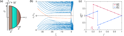
In this Letter, we will consider such a model and discuss a specific realization using a torus geometry (or smooth deformations thereof) as shown in Fig. 1, where the emerging hinge states are shown with blue and red arrows. This geometry allows us to insert a magnetic flux through the torus hole, and thus we construct a 3D analogy of the Corbino disc which is used in the Laughlin argument for the conventional 2D-QHE [51]. However, in contrast to the Corbino setup, the 3D-SOTI QHE discussed here is not induced by orbital effects but results purely from the Zeeman effect.
While there are several approaches known to deduce the conventional 2D quantized Hall conductance [51, 52, 53, 54], we will present a generalization of a recently developed boundary charge approach to the case of a 3D-SOTI, which, most importantly, is applicable to both clean and disordered systems. It is based on recent detailed studies of the boundary charge in one-dimensional (1D) modulated wires [55, 56, 57, 58, 59, 60, 61, 62, 63, 64, 65], together with dimensional extensions to 2D-QHE models [56, 57] revealing the fundamental relationship between the linear dependence of the boundary charge on the phase of the potential in 1D models and the quantized Hall conductance in 2D models, a concept which can even be generalized to explain the fractional QHE in the presence of interactions [62].
Most importantly, we demonstrate for the 3D-SOTI model on a torus that the boundary charge, driven by the Aharonov-Bohm flux , where is the flux quantum, shows a linear relation with respect to , with the slope being universal and quantized to integer numbers , where is the electron charge. Examining all states below the chemical potential, we reach a remarkable conclusion: the whole contribution to the boundary charge comes only from the top-most occupied valence band [shown in orange in Fig. 2(a)]. We further include disorder effects by considering a 3D tight-binding (tb) counterpart of our continuum model with broken rotational symmetry and show robustness of the quantized slope. The boundary charge concept, thus, provides a powerful tool in characterizing 3D-SOTIs and universally explains topological effects in condensed matter systems as well as their stability against random potential disorder and continuous surface deformations.
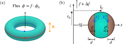
Model.—In this Letter we consider a continuum model in a finite three-dimensional region, which is confined to the interior of a torus [see Fig. 1(a))], to realize a second order TI with a minimal set of ingredients, given by band inversion, spin-orbit coupling, magnetic flux, and Zeeman term. The Hamiltonian (with ) is given by
| (1) |
where p and are 3D vectors of the momentum and the physical spin- operators, respectively. The parameters and are the effective mass of the electron and the spin-orbit interaction, respectively, while denotes the Zeeman energy. Both the magnetization direction inducing the Zeeman term and the uniform magnetic field B generated by the vector potential A are assumed to point along the -axis. We note that is an independent parameter, controllable by magnetic doping. The Pauli matrices span the orbital degrees of freedom. The parameter is chosen positive in order to realize the band inversion at finite values of , , and . The vector potential contains the terms generating both the uniform magnetic field and the Aharonov-Bohm (AB) magnetic flux . Here, we used the cylindrical coordinates and introduced the number of flux quanta .
Besides the spin-orbit length , we introduce two further typical scales and associated with the orbital magnetic field and the Zeeman term, respectively, via and . In the main part of this Letter we will discuss the most critical case of strong orbital fields, where , and will see that the orbital effects do not influence the quantization of the Hall conductance. In the Supplemental Material (SM) [66] we will also discuss the case of zero orbital effects with the same conclusion. This shows that our results are expected to be stable for any orbital field.
In the torus geometry and in the absence of disorder the model (1) possesses the axial symmetry generated by the -component of the total angular momentum operator . Exploiting this symmetry we reduce the 3D model to an effective 2D model. It is described by the Hamiltonian (see SM [66] for details)
| (2) |
and defined on the disc of radius in the half-plane, which is displaced away from the -axis by [see Fig. 1(b)]. We introduce the following continuous parameter , where are half-integer eigenvalues of the operator , and is restricted to fractional values, , interpolating between adjacent values of . The parameter appears inside the function , where the last term accounts for the orbital -field effect.
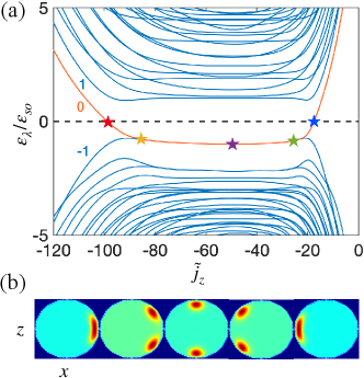
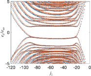
Hinge states.—Approximating (2) by its tight-binding (tb) lattice counterpart or by solving it directly in an appropriately chosen basis (see SM [66] for details), we calculate the band structure shown in Fig. 2(a). Among the valence and conduction bands , labeled by the band indices and and lying below and above the chemical potential , respectively, there is a distinguished band (orange line) which crosses the chemical potential at the two points (with ), see also in Fig. 4(a).
As shown in Fig. 2(b), the states on the negative linear slope near (indicated by the red star) form the right () hinge mode, since their density is localized near the disc right side (expressed in the polar coordinates , , with and , associated with the disc). They propagate in the clockwise direction along the outer equator of the torus (looking from the top), see the red line in Fig. 1(a). The left () hinge mode with the positive slope resides near [indicated by the blue star in Fig. 2(a)], its states are localized near (inner equator of the torus) and propagate in the counter-clockwise direction, see the blue line in Fig. 1(a).
To understand the properties of these hinge modes more deeply we rely on their low-energy description [66] which is valid in the regime and . It allows us to reveal the spinor structure of the hinge modes as well as to provide quantitative estimates of their properties.
In particular, we establish that the and hinge modes are stabilized by the Zeeman term, staying exponentially localized near the torus surface on the length scale of . In the angular direction, their localization is gaussian with the variance . The presence of in the variance is indicative of the Zeeman mechanism of their onset. Moreover, we notice that their angular spread exceeds the radial localization length, that is . Finally, we approximate the energy dispersion of the and hinge modes by , where the offsets account the -field flux quanta through the outer and inner equatorial rings of the torus, i.e. are generated by the orbital effects of the -field.
Plateau region.—In the broad range , there is a nearly degenerate plateau of weakly dispersing Landau surface states [between yellow and green stars in Fig. 2(a)]. Looking first at the states in the plateau’s middle (that is near the purple star in Fig. 2(a) at ), we observe that they are the linear combinations of the so called top and bottom Landau surface states that are localized near and , respectively. Due to the finite torus size, the splitting between and bands in the middle of the plateau is estimated by an exponentially small value [66]. The density of the state with higher energy, i.e. belonging to the band , is shown in the central inset of Fig. 2(b). This state is drastically different from the above discussed and hinge states, since its stabilization occurs due to the orbital -field effect, while the Zeeman term produces only a perturbative contribution to its energy. The low-energy analysis also predicts that its angular variance is both independent of and smaller than the variance of the and hinges (while the radial localization length remains the same).
The other states belonging to connect the top-bottom Landau surface states in the plateau middle with the and hinges on the linear branches of the band . Their density localization evolves along the disc circumference in the angular direction with the changing value [see Fig. 2(b)]. These states retain the same radial localization length , while their angular variances increase from the top-bottom Landau surface states to the and hinges, with the stabilization mechanism accordingly changing from the orbital to the Zeeman effect.
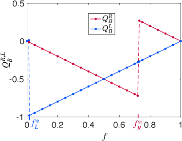
Boundary charge and 3D-SOTI QHE.—A convenient way to introduce the Hall conductance is to define it via the charge localized within an appropriately chosen boundary region [55, 56, 57, 58]. In our model, the outer () and the inner () boundary regions [shown in brown in Fig. 1(b)] are bounded by the cylindrical shells of the radii , respectively. Choosing the width such that , we ensure that the and hinge states are fully confined within , respectively. It is natural to define the boundary charges , with
| (3) |
where is a partial contribution of the state evaluated at the AB flux . To make the definition of for each band insensitive to a specific choice of , we subtract a large background contribution at zero flux.
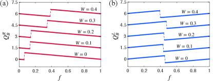
The central result of this Letter, supported by the numerical result shown in Fig. 3, is that the dependence of on the flux is piece-wise linear,
| (4) |
with jumps at , where is half-integer. The slope value is correlated with the jump size such that the periodicity is maintained. Changing the flux adiabatically in time, the immediate consequence of (4) is the quantization of the Hall conductance, relating the Hall current to the electric field via , see Fig. 1(b) and the discussion in Refs. [56, 57, 62]. Using Faraday’s law and the continuity equation we get and . Together with and , we obtain the quantization of the Hall conductance away from the jump points .
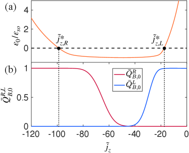
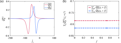
The second important result is that the contribution from all valence bands with is negligible (see SM [66] for the numerical verification). This is an intuitively expected result, since the valence band is separated from the band by the topologically trivial, though exponentially small, gap. The only contribution to the boundary charge is thus provided by the mode , which is shown in Fig. 4.
Let us provide the analytical arguments for the results presented above. Concerning the discrete jumps of at , it is obvious that they appear at those flux values, where a half-integer exists with . These are the points where the / hinge modes of the band cross the chemical potential, leading to a jump of by . In contrast, for all fully occupied bands , there is no jump.
The linear dependence on the flux follows essentially from the smooth behaviour of as function of , i.e., it varies typically on the scale of the plateau size, see Fig. 4(b) for (the same applies for all , except that the asymptotic values are coinciding). The plateau size is roughly related to the number of flux quanta threaded through the torus surface from the orbital field (for another scale is obtained, see SM [66]). Therefore, the -th order derivative of will scale with in the plateau region (outside this region the derivatives are very small), leading with an additional factor from the sum over to the scaling . Thus, all higher-order derivatives are negligible for , provided that is fulfilled. This can be achieved to any desired accuracy by increasing the torus radius (this result holds for any , see SM [66]). Therefore, only the linear term in contributes significantly to for each band. Since the slope value of the linear term of is correlated with the discrete jumps due to the periodicity property , we find that the slope is zero for all bands and for . This shows that the contribution of all valence bands is negligible and the universal linear slope of the total boundary charge is fully determined by the band.
Disorder effects.—We add random disorder potentials to every site of the 3D tb lattice realization of the Hamiltonian (1). Disorder breaks the rotational symmetry, the quantum number is no longer conserved, and the band index is not well defined either. Remarkably, the boundary charge , in which all the states below are included, is still well defined, as well as the relation between the boundary charge and the Hall conductance. In Fig. 5 we show that the linear slopes of remain very close to the universal value , i.e. staying essentially unaffected by disorder. This demonstrates the fundamental significance of the boundary charge concept: It is capable of explaining the Hall conductance quantization even in the disordered case, when the simple clean-case explanation presented above is no longer applicable.
Discussion.— The proposed 3D-SOTI QHE is robust to disorder which is very promising for its experimental realization using standard 3D-TIs with Zeeman fields induced by external magnetic fields, magnetic doping, or nearby ferromagnets. It occurs specifically only in 3D systems (for system sizes exceeding the localization length of hinge states) and is insensitive to orbital effects (see SM [66]), providing various fingerprints for its unique observation. Moreover, it is robust to shape distortions and will even occur in a spherical model with an infinitesimally thin hollow tube along the vertical axis (to allow for the Aharonov-Bohm flux insertion). The obtained results for the boundary charge showcase the same qualitative features as in the torus model (see SM [66]) and its detailed study opens another avenue of future research.
Acknowledgments.—This work was supported by the Deutsche Forschungsgemeinschaft via RTG 1995, the Swiss National Science Foundation (SNSF) and by the Deutsche Forschungsgemeinschaft (DFG, German Research Foundation) under Germany’s Excellence Strategy - Cluster of Excellence Matter and Light for Quantum Computing (ML4Q) EXC 2004/1 - 390534769. We acknowledge support from the Max Planck-New York City Center for Non-Equilibrium Quantum Phenomena. Simulations were performed with computing resources granted by RWTH Aachen University under projects rwth0752 and rwth0841, and at sciCORE (http://scicore.unibas.ch/) scientific computing center at University of Basel. Funding was received from the European Union’s Horizon 2020 research and innovation program (ERC Starting Grant, grant agreement No 757725).
Appendix A Effective low-energy theory
A.1 Derivation of the effective two-dimensional model by exploiting the rotational symmetry
Performing the unitary transformation , which transforms
| (9) | ||||
| (10) | ||||
| (11) |
supporting the periodic boundary conditions in , we obtain
| (12) | ||||
| (13) | ||||
| (14) |
By virtue of the transformation we remove the -dependence from the Hamiltonian and thereby explicitly manifest the rotational symmetry about axis, .
The total angular momentum operator can be replaced by its half-integer eigenvalue . Combining the latter with , we obtain the parameter . In addition, we perform the transformation
| (15) |
in order to have the euclidean scalar product in the effective two-dimensional model formulated in the half-plane . Finally, renaming , we obtain the Hamiltonian (2).
A.2 Coordinate transformation
The Hamiltonian (1) for the torus model can be alternatively represented in the new – toroidal-poloidal – coordinate system
| (16) | ||||
| (17) |
where and . Transforming the differential operators, we obtain
| (18) | ||||
| (19) |
where
| (20) |
In addition, the two-dimensional Laplace operator reads
| (21) |
Then, we rewrite (2) as
| (22) |
A.3 Matrix elements of the 2D model in the basis of Bessel functions
To compute matrix elements in the torus model we introduce the eigenbasis of with the open boundary conditions on the disc
| (23) |
It is expressed in terms of the Bessel function and its zeroes enumerated by for each . Being normalized by
| (24) |
the eigenfunctions (23) obey the orthogonality condition
| (25) |
Focusing on the representation (22), we analytically evaluate the matrix elements
| (26) | ||||
| (27) |
and numerically evaluate the matrix elements , , , .
Choosing an appropriate high-energy cutoff, we diagonalize the matrix Hamiltonian and compare its spectrum in Fig. 6 with the tb model spectrum presented in the main text.
A.4 Effective surface model
To derive an effective surface model, we apply the following unitary transformation to the Hamiltonian (22)
| (28) |
which maintains the periodic boundary conditions in variable.
The transformation (28) acts as follows:
| (29) | |||
| (30) | |||
| (31) | |||
| (32) |
and
| (33) |
The listed transformed operators are to replace in (22) their initial counterparts.
In addition to (28), we transform wavefunctions in order to absorb the functional determinant into the wavefunction’s definition. Accordingly we transform all operators, . Thus we get
| (34) |
For a sufficiently large radius , we can neglect the curvature effects in deriving the low-energy theory for surface states. Considering first the radial part of (34)
| (35) |
we establish that surface states are zero-energy states of this Hamiltonian, and their radial dependence is captured by the ansatz
| (36) |
with . Inserting it into (35), we obtain an equation for the spinor structure of the surface states
| (37) |
Hence we find the projector onto the surface states subspace
| (38) |
A.5 Hinge and Landau surface states in the torus model
1) To describe the right and left hinge states, we consider in the effective surface Hamiltonian (39) and derive
| (40) |
Near we approximate
| (41) |
At we solve the eigenvalue problem for a hinge state with nearly zero energy
| (42) |
Thus is a simultaneous eigenstate (to the eigenvalue ) of the projectors and . It reads
| (51) |
Noticing that , we perturbatively evaluate the energy dispersion in
| (52) |
Undoing the -transformation, we obtain
| (61) |
Note that .
2) To describe the top and bottom Landau surface states we consider the values , which correspond to the spatial localization at , that is or .
Carefully approximating
| (62) |
we extract the leading order Hamiltonian
| (63) |
It possesses the two zero-energy solutions: the top and bottom states with , which are localized near and , respectively. Their spinor structure is determined by the relations and :
| (72) |
Undoing the -transformation, we obtain
| (77) | ||||
| (82) |
Energy of these states is obtained from the perturbative -independent correction
| (83) |
The degeneracy is lifted by the exponentially small overlap of the two states, which leads to the symmetric and antisymmetric combinations of the top and bottom states. In particular, projecting the initially neglected small terms
| (84) |
onto the subspace spanned by the top and bottom states found above in the leading approximation, we obtain the following effective Hamiltonian
| (87) |
where
| (88) |
Diagonalizing (87), we obtain the energy splitting
| (89) |
It is minimal in the plateau’s middle,
| (90) |
giving an estimate of the splitting between and bands.
Appendix B Vanishing contribution to the boundary charge from the valence bands
Appendix C Details of the tight-binding modelling and calculation of the boundary charge
C.1 2D tight-binding model as a discrete version of the continuum model
To numerically solve the effective 2D continuum model shown in Eq. (2) of the main text, we first replace the continuous coordinates by discrete sites, and substitute the derivatives with finite differences [67]. The site labelled by has the position , where are integer numbers, is a lattice constant chosen to be small as compared to other scales in the model, and with is the unit vector pointing towards the -direction. In the lattice representation, the differential operators are replaced as: , and , where is the 2D wavefunction. With this approximation we get the matrix representation of the Hamiltonian (2) which is in the tb form and only contains the nearest coupling terms between adjacent sites. To get the geometry of a disc as shown in Fig. 1(b) of the main text, we consider a rectangular grid with length and width slightly larger than , and choose the center of the grid to coincide with that of the disc. By applying an infinitely large on-site potential outside the disc boundary, we achieve a realization of the open boundary conditions on the disc boundary. By exact diagonalization of the Hamiltonian matrix, we obtained the band structure, the density of states, and the boundary charge. In Fig. 6 we compare the low-energy states obtained from the 2D tb model by setting , and the one from directly solving the continuum model (2) in the basis introduced in the subsection A.3. The good agreement validates the accuracy of the 2D tb approximation.
C.2 Tight-binding Hamiltonian of the 3D TI under magnetic fields
To calculate the boundary charge in the presence of disorder potential, we use a 3D tb Hamiltonian of a TI [68, 69]. The Hamiltonian defined on a cubic lattice is written as
| (93) |
where is the Wannier basis denoting the lattice site with real-space position , and has both orbital and spin degrees of freedom encoded in the components with and . Here and represent the hopping amplitude and the lattice constant of the 3D tb model, respectively. The onsite matrix elements are given by , where is the dimensionless Zeeman energy in units of , and is the on-site disorder potential which is uniformly distributed within with being the characteristic disorder strength. The hopping matrix elements are given by .
The orbital effect of the magnetic field is included by adding a phase factor to the hopping matrices , with the vector potential containing contributions which generate both the uniform magnetic field and the AB flux. In the real calculations to get the geometry of a torus, we start with a cuboid of the size , and restrict the actual volume to the interior of the torus by applying an infinite onsite potential outside it. To simplify the numerical calculation we use the Landau gauge for , and the discontinuous gauge for .
Let us now relate the parameters of the above introduced 3D tb model to the parameters of the Hamiltonian (1) in the main text. To this end, we first omit in the 3D tb Hamiltonian the disorder term and the orbital effects of the magnetic fields, and relax the boundary conditions. This restores the translational invariance and allows us to introduce the Bloch Hamiltonian
| (94) |
with
| (95) |
Approximating this expression around the point in the Brillouin zone by the virtue of relations and , we get
| (96) |
To achieve the equivalence between (96) and (1), we identify , , , and . By setting the hopping energy and the lattice constant , we get the following values of the dimensionless parameters in the 3D tb Hamiltonian: and , in accordance with the parameter values of the Hamiltonian (1) specified in the caption of Fig. 2. The orbital effect of the magnetic field is incorporated by substituting with . The magnetic flux through each unit cell projected onto the plane generated by the uniform magnetic field is calculated to be . This observation helps us to calculate numerically the phase factor appearing in (93).
Having established the correspondence in the low-energy description between the 3D tb Hamiltonian and its continuum model counterpart, we further use the tb model to evaluate the boundary charge in the presence of on-site disorder breaking the rotational symmetry. The corresponding results are shown in Fig. 5 of the main text.
C.3 Green’s function method in calculating the boundary charge
Since we have used a 3D cuboid to simulate the torus model, the starting lattice has sites. Accounting the spin and orbital degrees of freedom, we obtain the Hilbert space dimension of the tb Hamiltonian to be . For the torus with and , we need at least , and . Exactly diagonalizing such a huge matrix of the dimension requires a large amount of virtual computer memory rendering the calculation very time-consuming. Instead of this direct approach, we adhere to the recursive Green’s function method [70] to calculate the boundary charge. This method allows us to separate the task into hundreds of jobs which can be computed in parallel on a high-performance computing cluster.
The total charge within the region below the chemical potential of the 3D lattice system is defined as: , where is the total charge at site . Here is the discrete eigenvalues of the isolated system with eigenstate , , and is the local density of states at site . Further, we represent
| (97) |
in terms of the site-diagonal components of the Green’s function . In this expression, a counterclockwise integration path in the complex- plane encompasses the poles of at lying below the chemical potential .
To facilitate the integration, we use a rectangular loop with the four corners in the complex plane: , and , where and are both large and positive real numbers denoting the absolute maximum values of the imaginary and real part of , respectively. This allows us to express
| (98) |
The last two integrals are insensitive to the parameter (which can be ever numerically tested), because they account contributions from the states lying far below the Fermi surface. This observation leads us to the operational formula
| (99) |
To calculate , we employ the recursive Green’s function method [70] which avoids a direct calculation of the inverse of the huge Hamiltonian matrix.
Appendix D 3D QHE in the absence of the orbital -field effect
In Fig. 8(a) we show the band structure of our model in the absence of the orbital -field effect. It features the two mid-gap modes of the and hinge states traversing the surface gap and connecting the hinge modes with bulk surface states. In Fig. 8(b) we show the right and left boundary charges (defined within the same boundary regions as in Fig. 1(b)) which receive contributions from all occupied states below the chemical potential . They feature the linear dependencies on with the slope values -0.9859 and 0.9523, which are complemented by the jumps of the corresponding sizes.
In the absence of the orbital -field effect there is no plateau region of surface states connecting the and hinges. Therefore for the analytical explanation it is easier to consider the total boundary charge and write it as a sum over all total angular momenta
| (100) |
where includes the sum over all bands and the condition that the energy must be smaller than
| (101) |
To estimate the typical scale on which is expected to vary on (up to jumps occurring when the energy of the highest valence band crosses the chemical potential), we have to compare the scale of the momentum parallel to the surface with various other inverse length scales appearing in the Hamiltonian (22) (like , , or ). Since all these inverse length scales are independent of , the scale will always increase with the torus radius and we find, analog to the arguments presented in the main text, that the boundary charge is dominated by its linear term to any desired degree of accuracy by increasing the torus radius. The linear behaviour together with the jump properties and the periodicity of then proves the universal slopes of in the same manner as discussed in the main text.
In the presence of strong orbital fields we note that the typical scale arises from the combination in the Hamiltonian (22). With and we get
| (102) |
The first term leads to an unimportant shift of . With and , the last two terms determine the scale which is of the order of the number of fluxes threaded through the torus surface from the orbital field, cf. the main text.
As a result, for any value of the orbital field , we obtain that the scale increases linearly with the torus radius . Therefore, the universal form of the boundary charge is unaffected by the orbital effects. We note that our estimate of the higher-order derivatives
| (103) |
is quite conservative. The reason is that the sum over for the higher-order derivatives , with , of (100) contains many terms with different signs which partially cancel each other. This can be seen from replacing sums by integrals and noting that the asymptotic values of , with , go to zero for . The same holds close to the point where the highest valence band leads to a jump of when some hinge modes crosses the chemical potential. The variation in becomes very weak close to the jumping point if the boundary region is chosen much larger than the localization length of all hinge modes. The vanishing integral of all higher-order derivatives with then indicates that also the sum is expected to be very small providing another reason why the linear behaviour is so robust with an error expected to be even much smaller than . This is indeed the case in Fig. 8, where , but the deviation from the linear behaviour is much smaller than .
Appendix E 3D QHE in the spherical geometry
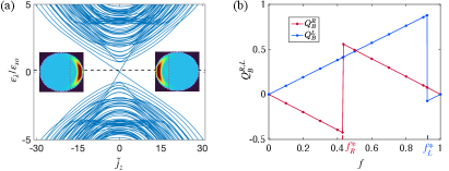
In Fig. 9 we show a two-dimensional projection of the sphere in the right half-plane appearing in the form of the half-disc. The model (with the magnetic orbital effects) is equipped with the open boundary conditions along its whole circumference including the vertical section. Vanishing of the wavefunction on the vertical section is equivalent to drilling an infinitesimally thin hole in the sphere, which allows for an insertion of the AB flux.
The band structure shown in Fig. 9(b) features a distinguished band (marked in orange) of states residing along the circumference of the half-disc. The states on the negative gentle slope are the hinge states localized near the spherical equator, while the states on the positive steep slope are spatially localized along the vertical axis.
In Fig. 9(c) the right and left boundary charges in the corresponding brown regions of the panel (a) are shown as functions of . They receive the whole contribution from the orange band of the panel (b). The calculated slopes are very close to the universal unit values, which is analytically explained by the same arguments as in the torus case.
References
- Klitzing et al. [1980] K. v. Klitzing, G. Dorda, and M. Pepper, New method for high-accuracy determination of the fine-structure constant based on quantized hall resistance, Phys. Rev. Lett. 45, 494 (1980).
- Kane and Mele [2005a] C. L. Kane and E. J. Mele, Quantum spin hall effect in graphene, Phys. Rev. Lett. 95, 226801 (2005a).
- Kane and Mele [2005b] C. L. Kane and E. J. Mele, topological order and the quantum spin hall effect, Phys. Rev. Lett. 95, 146802 (2005b).
- Bernevig et al. [2006] B. A. Bernevig, T. L. Hughes, and S.-C. Zhang, Quantum spin hall effect and topological phase transition in hgte quantum wells, Science 314, 1757–1761 (2006).
- König et al. [2007] M. König, S. Wiedmann, C. Brüne, A. Roth, H. Buhmann, L. W. Molenkamp, X.-L. Qi, and S.-C. Zhang, Quantum spin hall insulator state in hgte quantum wells, Science 318, 766 (2007).
- Hasan and Kane [2010] M. Z. Hasan and C. L. Kane, Colloquium: Topological insulators, Rev. Mod. Phys. 82, 3045 (2010).
- Qi and Zhang [2011] X.-L. Qi and S.-C. Zhang, Topological insulators and superconductors, Rev. Mod. Phys. 83, 1057 (2011).
- Haldane [1988] F. D. M. Haldane, Model for a quantum hall effect without landau levels: Condensed-matter realization of the ”parity anomaly”, Phys. Rev. Lett. 61, 2015 (1988).
- Liu et al. [2008] C.-X. Liu, X.-L. Qi, X. Dai, Z. Fang, and S.-C. Zhang, Quantum anomalous hall effect in quantum wells, Phys. Rev. Lett. 101, 146802 (2008).
- Bestwick et al. [2015] A. J. Bestwick, E. J. Fox, X. Kou, L. Pan, K. L. Wang, and D. Goldhaber-Gordon, Precise quantization of the anomalous hall effect near zero magnetic field, Phys. Rev. Lett. 114, 187201 (2015).
- Yu et al. [2010] R. Yu, W. Zhang, H.-J. Zhang, S.-C. Zhang, X. Dai, and Z. Fang, Quantized anomalous hall effect in magnetic topological insulators, Science 329, 61 (2010).
- Chang et al. [2013] C.-Z. Chang, J. Zhang, X. Feng, J. Shen, Z. Zhang, M. Guo, K. Li, Y. Ou, P. Wei, L.-L. Wang, Z.-Q. Ji, Y. Feng, S. Ji, X. Chen, J. Jia, X. Dai, Z. Fang, S.-C. Zhang, K. He, Y. Wang, L. Lu, X.-C. Ma, and Q.-K. Xue, Experimental observation of the quantum anomalous hall effect in a magnetic topological insulator, Science 340, 167 (2013).
- Checkelsky et al. [2014] J. G. Checkelsky, R. Yoshimi, A. Tsukazaki, K. S. Takahashi, Y. Kozuka, J. Falson, M. Kawasaki, and Y. Tokura, Trajectory of the anomalous hall effect towards the quantized state in a ferromagnetic topological insulator, Nature Physics 10, 731 (2014).
- Feng et al. [2015] Y. Feng, X. Feng, Y. Ou, J. Wang, C. Liu, L. Zhang, D. Zhao, G. Jiang, S.-C. Zhang, K. He, X. Ma, Q.-K. Xue, and Y. Wang, Observation of the zero hall plateau in a quantum anomalous hall insulator, Phys. Rev. Lett. 115, 126801 (2015).
- Kandala et al. [2015] A. Kandala, A. Richardella, S. Kempinger, C.-X. Liu, and N. Samarth, Giant anisotropic magnetoresistance in a quantum anomalous hall insulator, Nature Communications 6, 7434 (2015).
- Deng et al. [2020] Y. Deng, Y. Yu, M. Z. Shi, Z. Guo, Z. Xu, J. Wang, X. H. Chen, and Y. Zhang, Quantum anomalous hall effect in intrinsic magnetic topological insulator mnbi¡sub¿2¡/sub¿te¡sub¿4¡/sub¿, Science 367, 895 (2020).
- Liu et al. [2020] C. Liu, Y. Wang, H. Li, Y. Wu, Y. Li, J. Li, K. He, Y. Xu, J. Zhang, and Y. Wang, Robust axion insulator and chern insulator phases in a two-dimensional antiferromagnetic topological insulator, Nature Materials 19, 522 (2020).
- Ge et al. [2020] J. Ge, Y. Liu, J. Li, H. Li, T. Luo, Y. Wu, Y. Xu, and J. Wang, High-Chern-number and high-temperature quantum Hall effect without Landau levels, National Science Review 7, 1280 (2020).
- Riberolles et al. [2021] S. X. M. Riberolles, Q. Zhang, E. Gordon, N. P. Butch, L. Ke, J.-Q. Yan, and R. J. McQueeney, Evolution of magnetic interactions in sb-substituted , Phys. Rev. B 104, 064401 (2021).
- Yan et al. [2021] C. Yan, S. Fernandez-Mulligan, R. Mei, S. H. Lee, N. Protic, R. Fukumori, B. Yan, C. Liu, Z. Mao, and S. Yang, Origins of electronic bands in the antiferromagnetic topological insulator , Phys. Rev. B 104, L041102 (2021).
- Fukasawa et al. [2021] T. Fukasawa, S. Kusaka, K. Sumida, M. Hashizume, S. Ichinokura, Y. Takeda, S. Ideta, K. Tanaka, R. Shimizu, T. Hitosugi, and T. Hirahara, Absence of ferromagnetism in down to 6 k, Phys. Rev. B 103, 205405 (2021).
- Xu et al. [2021] B. Xu, Y. Zhang, E. H. Alizade, Z. A. Jahangirli, F. Lyzwa, E. Sheveleva, P. Marsik, Y. K. Li, Y. G. Yao, Z. W. Wang, B. Shen, Y. M. Dai, V. Kataev, M. M. Otrokov, E. V. Chulkov, N. T. Mamedov, and C. Bernhard, Infrared study of the multiband low-energy excitations of the topological antiferromagnet , Phys. Rev. B 103, L121103 (2021).
- Sitte et al. [2012] M. Sitte, A. Rosch, E. Altman, and L. Fritz, Topological insulators in magnetic fields: Quantum hall effect and edge channels with a nonquantized term, Phys. Rev. Lett. 108, 126807 (2012).
- Tang et al. [2019] F. Tang, Y. Ren, P. Wang, R. Zhong, J. Schneeloch, S. A. Yang, K. Yang, P. A. Lee, G. Gu, Z. Qiao, and L. Zhang, Three-dimensional quantum hall effect and metal–insulator transition in zrte5, Nature 569, 537 (2019).
- Xu et al. [2014] Y. Xu, I. Miotkowski, C. Liu, J. Tian, H. Nam, N. Alidoust, J. Hu, C.-K. Shih, M. Z. Hasan, and Y. P. Chen, Observation of topological surface state quantum hall effect in an intrinsic three-dimensional topological insulator, Nature Physics 10, 956 (2014).
- Schumann et al. [2018] T. Schumann, L. Galletti, D. A. Kealhofer, H. Kim, M. Goyal, and S. Stemmer, Observation of the quantum hall effect in confined films of the three-dimensional dirac semimetal , Phys. Rev. Lett. 120, 016801 (2018).
- Zhang et al. [2019] C. Zhang, Y. Zhang, X. Yuan, S. Lu, J. Zhang, A. Narayan, Y. Liu, H. Zhang, Z. Ni, R. Liu, E. S. Choi, A. Suslov, S. Sanvito, L. Pi, H.-Z. Lu, A. C. Potter, and F. Xiu, Quantum hall effect based on weyl orbits in cd3as2, Nature 565, 331 (2019).
- Benalcazar et al. [2017a] W. A. Benalcazar, B. A. Bernevig, and T. L. Hughes, Quantized electric multipole insulators, Science 357, 61 (2017a).
- Benalcazar et al. [2017b] W. A. Benalcazar, B. A. Bernevig, and T. L. Hughes, Electric multipole moments, topological multipole moment pumping, and chiral hinge states in crystalline insulators, Phys. Rev. B 96, 245115 (2017b).
- Song et al. [2017] Z. Song, Z. Fang, and C. Fang, -dimensional edge states of rotation symmetry protected topological states, Phys. Rev. Lett. 119, 246402 (2017).
- Langbehn et al. [2017] J. Langbehn, Y. Peng, L. Trifunovic, F. von Oppen, and P. W. Brouwer, Reflection-symmetric second-order topological insulators and superconductors, Phys. Rev. Lett. 119, 246401 (2017).
- Geier et al. [2018] M. Geier, L. Trifunovic, M. Hoskam, and P. W. Brouwer, Second-order topological insulators and superconductors with an order-two crystalline symmetry, Phys. Rev. B 97, 205135 (2018).
- Imhof et al. [2018] S. Imhof, C. Berger, F. Bayer, J. Brehm, L. W. Molenkamp, T. Kiessling, F. Schindler, C. H. Lee, M. Greiter, T. Neupert, and R. Thomale, Topolectrical-circuit realization of topological corner modes, Nature Physics 14, 925 (2018).
- Schindler et al. [2018] F. Schindler, A. M. Cook, M. G. Vergniory, Z. Wang, S. S. P. Parkin, B. A. Bernevig, and T. Neupert, Higher-order topological insulators, Science Advances 4, eaat0346 (2018).
- Trifunovic and Brouwer [2019] L. Trifunovic and P. W. Brouwer, Higher-order bulk-boundary correspondence for topological crystalline phases, Phys. Rev. X 9, 011012 (2019).
- Fu et al. [2021] B. Fu, Z.-A. Hu, and S.-Q. Shen, Bulk-hinge correspondence and three-dimensional quantum anomalous hall effect in second-order topological insulators, Phys. Rev. Research 3, 033177 (2021).
- Petrides and Zilberberg [2020] I. Petrides and O. Zilberberg, Higher-order topological insulators, topological pumps and the quantum hall effect in high dimensions, Phys. Rev. Research 2, 022049 (2020).
- Volpez et al. [2019] Y. Volpez, D. Loss, and J. Klinovaja, Second-order topological superconductivity in -junction rashba layers, Phys. Rev. Lett. 122, 126402 (2019).
- Laubscher et al. [2019] K. Laubscher, D. Loss, and J. Klinovaja, Fractional topological superconductivity and parafermion corner states, Phys. Rev. Research 1, 032017 (2019).
- Fu et al. [2007] L. Fu, C. L. Kane, and E. J. Mele, Topological insulators in three dimensions, Phys. Rev. Lett. 98, 106803 (2007).
- Xu et al. [2012] S.-Y. Xu, M. Neupane, C. Liu, D. Zhang, A. Richardella, L. Andrew Wray, N. Alidoust, M. Leandersson, T. Balasubramanian, J. Sánchez-Barriga, O. Rader, G. Landolt, B. Slomski, J. Hugo Dil, J. Osterwalder, T.-R. Chang, H.-T. Jeng, H. Lin, A. Bansil, N. Samarth, and M. Zahid Hasan, Hedgehog spin texture and berry’s phase tuning in a magnetic topological insulator, Nature Physics 8, 616 (2012).
- Rienks et al. [2019] E. D. L. Rienks, S. Wimmer, J. Sánchez-Barriga, O. Caha, P. S. Mandal, J. Růžička, A. Ney, H. Steiner, V. V. Volobuev, H. Groiss, M. Albu, G. Kothleitner, J. Michalička, S. A. Khan, J. Minár, H. Ebert, G. Bauer, F. Freyse, A. Varykhalov, O. Rader, and G. Springholz, Large magnetic gap at the dirac point in bi2te3/mnbi2te4 heterostructures, Nature 576, 423 (2019).
- Khalaf [2018] E. Khalaf, Higher-order topological insulators and superconductors protected by inversion symmetry, Phys. Rev. B 97, 205136 (2018).
- Plekhanov et al. [2019] K. Plekhanov, M. Thakurathi, D. Loss, and J. Klinovaja, Floquet second-order topological superconductor driven via ferromagnetic resonance, Phys. Rev. Research 1, 032013 (2019).
- Ren et al. [2020] Y. Ren, Z. Qiao, and Q. Niu, Engineering corner states from two-dimensional topological insulators, Phys. Rev. Lett. 124, 166804 (2020).
- Laubscher et al. [2020a] K. Laubscher, D. Chughtai, D. Loss, and J. Klinovaja, Kramers pairs of majorana corner states in a topological insulator bilayer, Phys. Rev. B 102, 195401 (2020a).
- Laubscher et al. [2020b] K. Laubscher, D. Loss, and J. Klinovaja, Majorana and parafermion corner states from two coupled sheets of bilayer graphene, Phys. Rev. Research 2, 013330 (2020b).
- Plekhanov et al. [2020] K. Plekhanov, F. Ronetti, D. Loss, and J. Klinovaja, Hinge states in a system of coupled rashba layers, Phys. Rev. Research 2, 013083 (2020).
- Plekhanov et al. [2021] K. Plekhanov, N. Müller, Y. Volpez, D. M. Kennes, H. Schoeller, D. Loss, and J. Klinovaja, Quadrupole spin polarization as signature of second-order topological superconductors, Phys. Rev. B 103, L041401 (2021).
- Jackiw and Rebbi [1976] R. Jackiw and C. Rebbi, Solitons with fermion number ½, Phys. Rev. D 13, 3398 (1976).
- Laughlin [1981] R. B. Laughlin, Quantized hall conductivity in two dimensions, Phys. Rev. B 23, 5632 (1981).
- Thouless et al. [1982] D. J. Thouless, M. Kohmoto, M. P. Nightingale, and M. den Nijs, Quantized hall conductance in a two-dimensional periodic potential, Phys. Rev. Lett. 49, 405 (1982).
- Avron et al. [1983] J. E. Avron, R. Seiler, and B. Simon, Homotopy and quantization in condensed matter physics, Phys. Rev. Lett. 51, 51 (1983).
- Kohmoto [1985] M. Kohmoto, Topological invariant and the quantization of the hall conductance, Annals of Physics 160, 343 (1985).
- Park et al. [2016] J.-H. Park, G. Yang, J. Klinovaja, P. Stano, and D. Loss, Fractional boundary charges in quantum dot arrays with density modulation, Phys. Rev. B 94, 075416 (2016).
- Thakurathi et al. [2018] M. Thakurathi, J. Klinovaja, and D. Loss, From fractional boundary charges to quantized hall conductance, Phys. Rev. B 98, 245404 (2018).
- Pletyukhov et al. [2020a] M. Pletyukhov, D. M. Kennes, J. Klinovaja, D. Loss, and H. Schoeller, Surface charge theorem and topological constraints for edge states: Analytical study of one-dimensional nearest-neighbor tight-binding models, Phys. Rev. B 101, 165304 (2020a).
- Pletyukhov et al. [2020b] M. Pletyukhov, D. M. Kennes, J. Klinovaja, D. Loss, and H. Schoeller, Topological invariants to characterize universality of boundary charge in one-dimensional insulators beyond symmetry constraints, Phys. Rev. B 101, 161106(R) (2020b).
- Pletyukhov et al. [2020c] M. Pletyukhov, D. M. Kennes, K. Piasotski, J. Klinovaja, D. Loss, and H. Schoeller, Rational boundary charge in one-dimensional systems with interaction and disorder, Phys. Rev. Research 2, 033345 (2020c).
- Miles et al. [2021] S. Miles, D. M. Kennes, H. Schoeller, and M. Pletyukhov, Universal properties of boundary and interface charges in continuum models of one-dimensional insulators, Phys. Rev. B 104, 155409 (2021).
- Müller et al. [2021] N. Müller, K. Piasotski, D. M. Kennes, H. Schoeller, and M. Pletyukhov, Universal properties of boundary and interface charges in multichannel one-dimensional models without symmetry constraints, Phys. Rev. B 104, 125447 (2021).
- Laubscher et al. [2021] K. Laubscher, C. S. Weber, D. M. Kennes, M. Pletyukhov, H. Schoeller, D. Loss, and J. Klinovaja, Fractional boundary charges with quantized slopes in interacting one- and two-dimensional systems, Phys. Rev. B 104, 035432 (2021).
- Weber et al. [2021] C. S. Weber, K. Piasotski, M. Pletyukhov, J. Klinovaja, D. Loss, H. Schoeller, and D. M. Kennes, Universality of boundary charge fluctuations, Phys. Rev. Lett. 126, 016803 (2021).
- Piasotski et al. [2021] K. Piasotski, M. Pletyukhov, C. S. Weber, J. Klinovaja, D. M. Kennes, and H. Schoeller, Universality of abelian and non-abelian wannier functions in generalized one-dimensional aubry-andré-harper models, Phys. Rev. Research 3, 033167 (2021).
- Hayward et al. [2021] A. L. C. Hayward, E. Bertok, U. Schneider, and F. Heidrich-Meisner, Effect of disorder on topological charge pumping in the rice-mele model, Phys. Rev. A 103, 043310 (2021).
- [66] In the Supplemental Material we discuss the dimensional reduction of the 3D model; check the agreement of the low-energy state values in the effective 2D model between the tb and the continuum model calculations; provide the low-energy description of the hinge states; numerically verify the absent contribution to the linear slope from the bands , and provide theoretical details of the numerical studies in 3D tb model in the presence of the disorder potential. We also investigate the role of the orbital -field effect and deformations of the torus surface, showing the robustness of the discussed 3D QHE.
- Datta [1995] S. Datta, Electronic transport in mesoscopic systems (Cambridge university press, Cambridge, 1995) pp. 141–145.
- Shen [2017] S.-Q. Shen, Topological insulators: Dirac equation in condensed matters, second edition (Springer Nature Singapore Pte Ltd, Singapore, 2017).
- Hosur et al. [2011] P. Hosur, P. Ghaemi, R. S. Mong, and A. Vishwanath, Majorana modes at the ends of superconductor vortices in doped topological insulators, Phys. Rev. Lett. 107, 097001 (2011).
- Do [2014] V.-N. Do, Non-equilibrium green function method: theory and application in simulation of nanometer electronic devices, Advances in Natural Sciences: Nanoscience and Nanotechnology 5, 033001 (2014).