Real-time Path Planning of Driver-less Mining Trains with Time-dependent Physical Constraints

Define a physical network $G^{*}=(S,W)$ with a set of nodes S and a set of links W. The set S consists of switch stations ($S_{u}\subset S$), and load-outs ($S_{l}\subset S$) in physical network. $W=\{(i,j)\}$ is the set of links in physical network, where $(i,j)$ stands for link connecting node $i\in S$ to node $j\in S$. The set W consists of mainline tracks ($W_{u}\subset W$), siding tracks ($W_{w}\subset W$) and crossovers ($W_{o}\subset W$) in physical network. For each link $(i,j)$, let

• •

  $d_{ij}$ be the capacity of $(i,j)$: Here capacity is the maximum number of trains that can stand on the link $(i,j)$ at any point of time.

• •

  $f(i,j)$ be the travel time from i to j, where f is the speed profile based function.

• •

  $f(j,i)$ be the travel time from j to i, where f is the speed profile based function.

In order to model the business operation of mine loading, for each load-out $i\in S_{l}$, let $P_{i}$ be the average loading time for a train.

Let $Q=\{0,1,\cdots,|Q|-1\}$ be the set of time instants, where time is discretized into discrete time instants of length g minutes. For instance if we take g = 5 then a period of 1 hour would be represented by discrete set $Q=\{0,1,2,\cdots,12\}$ in our model.

Let $M=\{1,2,\cdots,m\}$ be the set of real trains travelling in the physical network $G^{*}$. For each train $m\in M$,we will get the following set of inputs:

• •

  $loSeq^{m}$: Sequence of scheduled load-outs to visit.

• •

  $depTime^{m}$: Scheduled departure time.

• •

  $depLoc^{m}$: Scheduled departure location.

As we have a cyclical network and train changes direction (turns back) after going to a load-out, in order to model this behaviour we will break down the train journey into different parts. Each part will be represented by a different model train. Thus, if a train $m$ goes to $n$ load-outs, its whole journey will be represented by a set of $n+1$ model trains called $T_{m}$, where each model train represents a specific segment of train $m$’s journey. Accordingly, one business rule will be added that any model train can depart only after its predecessor has finished its journey.

For example, considering the case of a train $m$ starting from station A and going to two load-outs G1 and G2, its journey will be modelled as follows:

From now on, we will use train to refer to model train only, unless specified otherwise. Thus, for each train $t\in T$, we will have the following set of information:

• •

  $depQ_{t}$: Scheduled departure time.

• •

  $dep_{t}$: Scheduled departure location node.

• •

  $dest_{t}$: Final destination node of the train, after which it will disappear from the network.

• •

  $t_{pre}$: Predecessor train of train t.

We here consider a time-space network $G=(N,A)$, where N denotes the node set and A denotes the arc set. For each node $i\in N$, let $Outb_{i}\subseteq A$ be the set of all the outbound arcs of node $i$, and $Inb_{i}\subseteq A$ be the set of all the inbound arcs of node $i$.

Given a physical network $G^{*}$, we then can construct the time-space network $G$ as follows:

• •

  For each load-out in $s\in S_{l}$, we replace it with two separate node $s_{in}$ (entry node) and $s_{out}$ (exit node), and add a load-out link ($s_{in}$, $s_{out}$) into W. Let $W_{l}\subset W$ be the set of load-out links. By splitting the entry and exit point nodes for each load-out, we ensure that trains are staying at load-out for the required loading time. At the same time, we replace the related inbound links $(i,s)\in W$ to $(i,s_{in})$ and the related outbound links $(s,j)\in W$ to $(s_{out},j)$. Accordingly, we have $f(i,s_{in})=f(i,s)$, $f(j,s_{out})=f(j,s)$, and $f(s_{in},s_{out})=P_{s}$, where $P_{s}$ indicates the required loading time.

• •

  For each link $(i,j)\in W$ whose capacity $d_{ij}>1$, we break down this link into smaller links by adding $\lfloor d_{ij}-1\rfloor$ dummy nodes into S and replacing the link $(i,j)$ with $\lfloor d_{ij}-1\rfloor$ dummy links (with proportional travel time) as well. Note: After this operation, the capacity of each arc is 1. This operation guarantees that on every arc at any point of time only one train travels on that arc, which will in turn guarantee that trains maintain a safe headway separation while travelling in the same direction.

• •

  For each siding track $(i,j)\in W_{w}$, we add a siding node $i^{\prime}$ to $S$ and replace the siding track $(i,j)$ with two separate arcs $(i,i^{\prime})$ and $(i^{\prime},j)$. Let $S_{w}\subset S$ be the set of siding nodes. Accordingly, we have $f(i,i^{\prime})=f(i^{\prime},j)=f(i,j)/2$ and $f(j,i^{\prime})=f(i^{\prime},i)=f(j,i)/2$. For each link $(i,j)\in W$, let $Iden(i,j)$ be the set of identical arcs in $A$.

• •

  For each node $s\in S$, we add $|Q|$ corresponding nodes $\{s^{0},...,s^{|Q|-1}\}$ in $N$. For each train $t\in T$, we add corresponding virtual source node $s_{0}^{t}$ in $N_{s}\in N$, where $s_{0}^{t}$ represents the source node where train $t$ departs. We also add one sink $s_{1}$ into $N$, where $s_{1}$ represents the sink node where every train terminates its journey.

• •

  For each link $(i,j)\in W$, we add following transit arcs into $Iden(i,j)\subset A$:

  $$(i^{k},j^{k+f(i,j)}),\ for\ all\ k=0,...,|Q|-1\ and\ k+f(i,j)\leq|Q|-1$$

  $$(j^{k},i^{k+f(j,i)}),\ for\ all\ k=0,...,|Q|-1\ and\ k+f(j,i)\leq|Q|-1$$

• •

  For each link $(i,i^{{}^{\prime}})\in W_{w}$, we then update $Iden(i,i^{{}^{\prime}})$ as follows:

  $$Iden(i,i^{{}^{\prime}})=Iden(i^{{}^{\prime}},j)=Iden(i,i^{{}^{\prime}})\cup Iden(i^{{}^{\prime}},j)$$

• •

  For each siding node $i\in N$, we add following waiting arcs into $A_{w}\subset A$. In this way, we allow trains to wait/dwell on sidings.

  $$(i^{k},i^{k+1}),\ for\ all\ k=0,...,|Q|-2$$

• •

  For any load-out $s\in S_{l}$ with loop capacity $cap_{s}$, we add $(cap_{s}-1)$ waiting arcs between $(s_{in}^{k},s_{out}^{k})$ , for all $k=0,...,|Q-2|$. In this way, we allow trains to wait/dwell in the loops.

• •

  For each station node $i\in S_{u}$, we add an arc from that node to the sink, signifying that allows train cancelling in case of deadlock (i.e. we can cancel a train with a very high penalty). Thus we add these train disappearing arcs into $A_{d}\subset A$:

  $$(i^{k},s_{1}),\ for\ all\ k=0,...,|Q|-1$$

• •

  For each train $t\in T$, we add an arc from the source to the scheduled starting node of that train, and we add these starting arcs into $A_{s}\subset A$:

  $$(s_{0}^{t},j^{k}),\ for\ all\ k\geq depQ_{t},\ and\ j\ is\ the\ scheduled\ starting\ node(i.e.,\ j=dep_{t})$$

• •

  In all the above cases, whenever an arc $(i,j)\in A$ is added to the time-space network, we also add this arc to the Outbound arc set of node $i(i.e.Outb_{i})$ and to the Inbound arc set of node $j(i.e.Inb_{j})$.

For each $(i^{k},j^{l})\in A$ and a given train $t\in T$, there exists a cost attribute $c^{t}_{i^{k}j^{l}}$ as follows:

where $(i^{k},j^{l})$ denotes an arc in the time space network representing possible movement (of a train) starting from node $i$ at time $k$ and terminating at node $j$ at time $l$. The cost $\alpha*(|Q|-\lfloor k/(60/g)\rfloor)$ implies that we give weighted penalties for waiting/dwelling, where $\alpha$ is constant parameter. The cost $\beta*(l-depQ_{t})$ implies the penalty for late departure, where $\beta$ is constant parameter. The cost $\rho*time_{left}$ implies that we try to route trains as close as to the destination. The cost $\gamma*(l-k)$ implies that we try to route trains along the shortest-time path.

For each $(i^{k},j^{l})\in A$ and a given train $t\in T$, define the following binary decision variable:

Given the above cost attributes and variables, we then define the objective as follows:

In particular, we formulate the related constraints as follows:

• •

  Flow conservation constraint: These constraints algebraically state that the sum of the flow through arcs directed toward a node plus that node’s supply, if any, equals the sum of the flow through arcs directed away from that node plus that node’s demand, if any.

  $$\sum_{(s^{t}_{0},j)\in Outb_{s^{t}_{0}}}x^{t}_{s_{0}^{t}j}=1,\forall t\in T$$

  $$\sum_{(i,s_{1})\in Inb_{s_{1}}}x^{t}_{is_{1}}=1,\forall t\in T$$

  $$\sum_{(i,j)\in Outb_{i}}x^{t}_{ij}-\sum_{(j,i)\in Inb_{i}}x^{t}_{ji}=0,\forall i\in N-N_{s}-\{s_{1}\},\forall t\in T$$

• •

  Node capacity constraint: This constraint ensures that for each node excluding $s_{1}$, trains can be held safely without any collision or deadlock at any time point.

  $$\sum_{t\in T}\sum_{(j,i)\in Inb_{i}}x^{t}_{ji}\leq 1,\forall i\in N-\{s_{1}\}$$

• •

  Arc capacity constraint: This constraint implies that for any track, load-out in the network, at any time instant $q\in Q$, there can only be at max one train travelling or staying.

  $$\sum_{t\in T}\sum_{(i^{{}^{\prime}k},j^{{}^{\prime}l})\in Iden(i,j)\&\{k\leq q-1,l\geq q\}}x^{t}_{i^{{}^{\prime}k}j^{{}^{\prime}l}}\leq 1,\forall q\in Q,\forall(i,j)\in W$$

• •

  Train departure constraint: This constraint implies that any train $t$ with predecessor not null, which represents the return trip of a real train, has to depart at the time when its predecessor train completes its journey.

  $$x^{t}_{s^{t}_{0}dep^{q}_{t}}-x^{t_{pre}}_{dest^{q}_{t}s_{1}}=0,\forall q\in[depQ_{t},Q],\forall t\in T\&t_{pre}\neq null$$

In the pre-processing step, we use the current status as input, and formulate the above MIP problem, which complexity changes exponentially when variable size varies. To further reducing the running time, we adopt the following approaches to reduce the variables:

• •

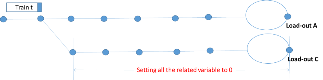
  Initializing variables only for arcs on which train will travel: for each train, we only consider the reasonable arcs according to its destination. For example, in fig. 3 the train $t$ is heading for load-out A. We then can set all the unreasonable variables (i.e., those variables associated to the arcs heading for load-out C) to 0.

• •

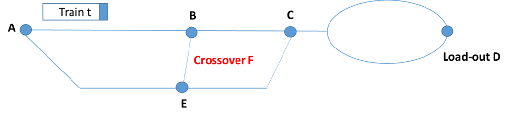
  Removing variables corresponding to unrealistic movements: consider the train $t$ in fig. 4 going towards load-out, which is not allowed to move on track F. We then fix variables corresponding to such invalid movements to 0.

In this step, we solve the formulated MIP problem via mathematical optimisation solver (e.g. Gurobi, Xpress, Cplex, etc). To better utilize the solver, we also integrate more strategies as follows:

• •

  Warm start: supply hints to help solver find an initial solution, which consist of pairs of variables and values, known as a warm start. The hints may come from soft business rules or human experience.

• •

  Solver tuning: use offline data to tune the solver, and adopt the solver setting for the online running.

After getting the MIP results, we then need to translate the math-style results into trains’ schedule solution. In particular, we need to combine trains with the related predecessor trains to get complete movements. As shown in table 1, we need to combine the results of $t_{m1}$, $t_{m2}$, $t_{m2}$ to get the schedule of train $m$.

For each given solution, we then validate the schedule further via simulation, and add more details including maintenance allocation. We finally trigger an actual execution by communicating the detailed schedule to trains.

We here consider the sample network in fig. 1, and has track capacity shown in fig. 5. As per the subsection 3.3, we then construct the time-space network of 20-minute time window in fig. 6, for which the time instant length is 5 minutes.

We then evaluate the proposed solution via the following test cases. From case 1 to case 4, we vary trains to schedule, generate the train schedule, and demonstrate the solution in time-space network.

Given a single train info in table 2, we are able to get the solution in less than one minute, where the train schedule for train Mtest01 is demonstrated via green-path in fig. 7.

We have two trains to schedule in table 3, where train Mtest01 goes towards load-out G and train Mtest02 returns from load-out G. We are able to get the solution in less than one minute, where the train schedule for train Mtest01/Mtest02 are demonstrated via green-path/blue-path respectively in fig. 8.

We have three trains to schedule in table 4: both train Mtest01 and Mtest03 go towards load-out G from different start station; train Mtest02 goes back from load-out G with departure time constraint. We are able to get the solution in less than one minute, and the train schedule are demonstrated via in fig. 9. In particular, train Mtest01/Mtest02/Mtest03 schedule are demonstrated via green-path/blue-path/orange-path respectively.

Given three trains info in table 5, both train Mtest01 and Mtest03 go towards load-out G with same start station; train Mtest02 goes back from load-out G with departure time constraint. Similar to case 3, we are able to get the solution in less than one minute, and demonstrate the train schedule in fig. 10, where train Mtest01/Mtest02/Mtest03 schedule are showed via green-path/blue-path/orange-path respectively.

References

- [1] C. Bersani, M. A. D. C. Estil-Les and R. Sacile, “Min-Max Approach for High-Speed Train Scheduling and Rescheduling Models,” in IEEE Access, vol. 9, pp. 41042-41051, 2021.
- [2] Ralf Borndörfer, Torsten Klug, Thomas Schlechte, Armin Fügenschuh, Thilo Schang and Hanno Schülldorf, “The Freight Train Routing Problem for Congested Railway Networks with Mixed Traffic,” in Transp.Sci., vol.50, no.2, pp. 408-423, May 2016.
- [3] N. Bešinović, B. Widarno and R. M. P. Goverde, “Adjusting freight train paths to infrastructure possessions,” 2020 IEEE 23rd International Conference on Intelligent Transportation Systems (ITSC), 2020.
- [4] V. Cacchiani, F. Furini and M.P. Kidd, “Approaches to a real-world train timetabling problem in a railway node,” in Omega, vol.58, pp. 97-110, 2016.
- [5] V. Cacchiani and P. Toth, “Nominal and robust train timetabling problems,” in Eur. J. Oper. Res., vol. 219, no. 3, pp. 727–737, Jun. 2012.
- [6] T. Ghasempour and B. Heydecker, “Adaptive railway traffic control using approximate dynamic programming,” in Transportation Research Part C: Emerging Technologies, vol.113, pp. 91-107, 2020.
- [7] S. Harrod, “Modeling network transition constraints with hypergraphs,” in Transp. Sci., vol. 45, no. 1, pp. 81–97, Feb. 2011.
- [8] S. Harrod, “A tutorial on fundamental model structures for railway timetable optimization,” in Surv. Oper. Res. Manage. Sci., vol. 17, no. 2, pp. 85–96, Jul. 2012.
- [9] P. Huang, C. Kung and C. Lin, “An Integrated Formulation and Optimization for Periodic Timetabling of Railway Systems,” 2021 IEEE International Intelligent Transportation Systems Conference (ITSC), 2021.
- [10] Z. Hou, M. Zhou, L. Ning and H. Dong, “Automatic Train Regulation with Time Tuning and Holding Control under the Saturated Passenger Demand Condition,” 2021 33rd Chinese Control and Decision Conference (CCDC), 2021.
- [11] L. Kang and Q. Meng, “Two-phase decomposition method for the last train departure time choice in subway networks,” in Transp. Res. B, Methodol., vol. 104, pp. 568–582, Oct. 2017.
- [12] L. Kang, J. Wu, H. Sun, X. Zhu, and B. Wang, “A practical model for last train rescheduling with train delay in urban railway transit networks,” in Omega, vol. 50, pp. 29–42, 2015.
- [13] L. Kang, J. Wu, H. Sun, X. Zhu and Z. Gao, “A case study on the coordination of last trains for the beijing subway network,” in Transp. Res. B, Methodol., vol. 72, pp. 112–127, Feb. 2015.
- [14] L. Kang, X. Zhu, H. Sun, J. Puchinger, M. Ruthmair and B. Hu, “Modeling the first train timetabling problem with minimal missed trains and synchronization time differences in subway networks,” in Transp. Res. B, Methodol., vol. 93, pp. 17–36, Nov. 2016.
- [15] S. Li, H. Lv, C. Xu, T. Chen and C. Zou, “Optimized Train Path Selection Method for Daily Freight Train Scheduling,” in IEEE Access, vol. 8, pp. 40777-40790, 2020.
- [16] R. Liu, S. Li and L. Yang, “Collaborative optimization for metro train scheduling and train connections combined with passenger flow control strategy,” in Omega, vol. 90, 101990, 2020.
- [17] Z. Li, B. Mao, Y. Bai and Y. Chen, “Integrated optimization of train stop planning and scheduling on metro lines with express/local mode,” in IEEE Access, vol. 7, pp. 88534–88546, Jun. 2019.
- [18] S. Mu and M. Dessouky, “Scheduling freight trains traveling on complex networks,” in Transp. Res. B, Methodol., vol. 45, no. 7, pp. 1103–1123, 2011.
- [19] H. Niu, X. Zhou and R. Gao, “Train scheduling for minimizing passenger waiting time with time-dependent demand and skip-stop patterns: Nonlinear integer programming models with linear constraints,” in Transportation Research Part B, vol. 76, pp. 117-135, 2015.
- [20] G. Polinder, T. Breugem, T. Dollevoet and G. Maróti, “An adjustable robust optimization approach for periodic timetabling,” in Transportation Research Part B: Methodological, vol. 128, pp. 50-68, 2019.
- [21] O. Ozturk and J. Patrick, “An optimization model for freight transport using urban rail transit,” European Journal of Operational Research, vol.267, issue.3, pp. 1110-1121, 2018.
- [22] J. Qi, S. Li, Y. Gao, K. Yang and P. Liu, “Joint optimization model for train scheduling and train stop planning with passengers distribution on railway corridors,” in J. Oper. Res. Soc., vol. 69, no. 4, pp. 556-570, Jan. 2018.
- [23] R. Sanat, T. Dutt, A. Chandrababu, A. Abhilasha and G. N. S. Prasanna, “Optimizing Schedule of Trains in Context of a Large Railway Network,” 2018 21st International Conference on Intelligent Transportation Systems (ITSC), 2018
- [24] K. Sato and N. Fukumura, “Real-time freight locomotive rescheduling and uncovered train detection during disruption,” in European Journal of Operational Research, vol.221, issue.3, pp. 636-648, 2012.
- [25] D. Sparing and R. Goverde, “A cycle time optimization model for generating stable periodic railway timetables,” in Transportation Research Part B: Methodological, vol.98, pp. 198-223, 2017.
- [26] P. Schiewe and A. Schöbel, “Periodic Timetabling with Integrated Routing: Toward Applicable Approaches,” in Transp.Sci.,vol. 54, no.6, pp. 1714-1731, Sep. 2020.
- [27] Y. Wang, A. D’Ariano, J. Yin, L. Meng, T. Tang and B. Ning, “Passenger demand oriented train scheduling and rolling stock circulation planning for an urban rail transit line,” in Transportation Research Part B: Methodological, vol. 118, pp. 193-227, DEC., 2018.
- [28] Y. Wu, H. Yang, S. Zhao and P. Shang, “Mitigating unfairness in urban rail transit operation: A mixed-integer linear programming approach,” in Transportation Research Part B: Methodological, vol.149, pp. 418-442, 2021.
- [29] Z. Wang, S. Su, B. Su and T. Tang, “A metro train rescheduling approach considering flexible short-turning and adding backup trains strategies during disruptions in the case of the vehicle breakdown,” 2021 IEEE International Intelligent Transportation Systems Conference (ITSC), 2021.
- [30] P. Xu, G. Feng, D. Cui, X. Dai, Q. Zhang and F. Chen, “Timetable Mapping Model and Dynamic Programming Approach for High-speed Railway Rescheduling,” 2020 39th Chinese Control Conference (CCC), 2020.
- [31] W. Xu, B. Xie, X. Zhang and L. Ning, “Timetable Rescheduling Considering Headway: A Genetic Algorithm Combined with the Benchmark Time Method,” 2020 IEEE 5th International Conference on Intelligent Transportation Engineering (ICITE), 2020.
- [32] J. Yin, D. Andrea, Y. Wang, J. Xun, S. Su and T. Tang, “Mixed-Integer Linear Programming Models for Coordinated Train Timetabling with Dynamic Demand,” 2019 IEEE Intelligent Transportation Systems Conference (ITSC), 2019
- [33] J Yin, T Tang et al., “Energy-efficient metro train rescheduling with uncertain time-variant passenger demands: An approximate dynamic programming approach,” in Transportation Research: Part B, vol.91, pp. 178-210, 2016.
- [34] Y. Zhu and R.Goverde, “Railway timetable rescheduling with flexible stopping and flexible short-turning during disruptions,” in Transportation Research Part B: Methodological, vol. 123, pp. 149-181, 2019.
- [35] J.-H. Zhong, M. Shen, J. Zhang, H. S.-H. Chung, Y.-H. Shi and Y. Li, “A Differential Evolution Algorithm With Dual Populations for Solving Periodic Railway Timetable Scheduling Problem,” in IEEE Transactions on Evolutionary Computation, vol. 17, no. 4, pp. 512-527, Aug. 2013.