Real-Time Numerical Differentiation of Sampled Data Using Adaptive Input and State Estimation
Abstract
Real-time numerical differentiation plays a crucial role in many digital control algorithms, such as PID control, which requires numerical differentiation to implement derivative action. This paper addresses the problem of numerical differentiation for real-time implementation with minimal prior information about the signal and noise using adaptive input and state estimation. Adaptive input estimation with adaptive state estimation (AIE/ASE) is based on retrospective cost input estimation, while adaptive state estimation is based on an adaptive Kalman filter in which the input-estimation error covariance and the measurement-noise covariance are updated online. The accuracy of AIE/ASE is compared numerically to several conventional numerical differentiation methods. Finally, AIE/ASE is applied to simulated vehicle position data generated from CarSim.
keywords:
Numerical differentiation, input estimation, Kalman filter, adaptive estimation1 Introduction
The dual operations of integration and differentiation provide the foundation for much of mathematics. From an analytical point of view, differentiation is simpler than integration; consider the relative difficulty of differentiating and integrating In numerical analysis, integration techniques have been extensively developed in Davis \BBA Rabinowitz (\APACyear1984), whereas differentiation techniques have been developed more sporadically in Savitzky \BBA Golay (\APACyear1964); Cullum (\APACyear1971), Hamming (\APACyear1973, pp. 565, 566).
In practice, numerical integration and differentiation techniques are applied to sequences of measurements, that is, discrete-time signals composed of sampled data. Although, strictly speaking, integration and differentiation are not defined for discrete-time signals, the goal is to compute a discrete-time “integral” or “derivative” that approximates the true integral or derivative of the pre-sampled, analog signal.
In addition to sampling, numerical integration and differentiation methods must address the effect of sensor noise. For numerical integration, constant noise, that is, bias, leads to a spurious ramp, while stochastic noise leads to random-walk divergence. Mitigation of these effects is of extreme importance in applications such as inertial navigation as shown in Farrell (\APACyear2008); Grewel \BOthers. (\APACyear2020).
Compared to numerical integration, the effect of noise on numerical differentiation is far more severe. This situation is due to the fact that, whereas integration is a bounded operator on a complete inner-product space, differentiation is an unbounded operator on a dense subspace. Unboundedness implies a lack of continuity, which is manifested as high sensitivity to sensor noise. Consequently, numerical differentiation typically involves assumptions on the smoothness of the signal and spectrum of the noise as considered in Ahn \BOthers. (\APACyear2006); Jauberteau \BBA Jauberteau (\APACyear2009); Stickel (\APACyear2010); Listmann \BBA Zhao (\APACyear2013); Knowles \BBA Renka (\APACyear2014); Haimovich \BOthers. (\APACyear2022).
Numerical differentiation algorithms are crucial elements of many digital control algorithms. For example, PID control requires numerical differentiation to implement derivative action as presented in Vilanova \BBA Visioli (\APACyear2012); Astrom \BBA Hagglund (\APACyear2006). Flatness-based control is based on a finite number of derivatives as shown in Nieuwstadt \BOthers. (\APACyear1998); Mboup \BOthers. (\APACyear2009).
In practice, analog or digital filters are used to suppress the effect of sensor noise, thereby allowing the use of differencing formulae in the form of inverted “V” filters, which have the required gain and phase lead at low frequencies and roll off at high frequencies. These techniques assume that the characteristics of the signal and noise are known, thereby allowing the user to tweak the filter parameters. When the signal and noise have unknown and possibly changing characteristics, filter tuning is not possible and thus the problem becomes significantly more challenging. The recent work in Van Breugel \BOthers. (\APACyear2020) articulates these challenges and proposes a Pareto-tradeoff technique for addressing the absence of prior information. Additional techniques include high-gain observer methods, in which the observer approximates the dynamics of a differentiator as shown in Dabroom \BBA Khalil (\APACyear1999). An additional approach to this problem is to apply sliding-mode algorithms as shown in Levant (\APACyear2003); Reichhartinger \BBA Spurgeon (\APACyear2018); López-Caamal \BBA Moreno (\APACyear2019); Mojallizadeh \BOthers. (\APACyear2021); Alwi \BBA Edwards (\APACyear2013).
In feedback control applications, which require real-time implementation, phase shift and latency in numerical differentiation can lead to performance degradation and possibly instability. Phase shift arises from filtering, whereas latency arises from noncausal numerical differentiation, that is, numerical differentiation algorithms that require future data. For real-time applications, a noncausal differentiation algorithm can be implemented causally by delaying the computation until the required data are available. A feedback controller requires an estimate of the current derivative, however, and thus the delayed estimate provided by a noncausal differentiation algorithm may not be sufficiently accurate.
A popular approach to numerical differentiation is to apply state estimation with integrator dynamics, where the state estimate includes an estimate of the derivative of the measurement as shown in Kalata (\APACyear1984); Bogler (\APACyear1987). This approach has been widely used for target and vehicle tracking in Jia \BOthers. (\APACyear2008); H. Khaloozadeh (\APACyear2009); Lee \BBA Tahk (\APACyear1999); Rana \BOthers. (\APACyear2020). As an extension of this approach, the present paper applies input estimation to numerical differentiation, where the goal is to estimate the input as well as the state, as in Gillijns \BBA De Moor (\APACyear2007); Orjuela \BOthers. (\APACyear2009); Fang \BOthers. (\APACyear2011); Yong \BOthers. (\APACyear2016); Hsieh (\APACyear2017); Naderi \BBA Khorasani (\APACyear2019); Alenezi \BOthers. (\APACyear2021).
The present paper is motivated by the situation where minimal prior information about the signal and noise is available. This case arises when the spectrum of the signal changes slowly or abruptly in an unknown way, and when the noise characteristics vary due to changes in the environment, such as weather. With this motivation, adaptive input estimation (AIE) was applied to target tracking in Ansari \BBA Bernstein (\APACyear2019), where it was used to estimate vehicle acceleration using position data. In particular, the approach of Ansari \BBA Bernstein (\APACyear2019) is based on retrospective cost input estimation (RCIE), where recursive least squares (RLS) is used to update the coefficients of the estimation subsystem. The error metric used for adaptation is the residual (innovations) of the state estimation algorithm, that is, the Kalman filter. This technique requires specification of the covariances of the process noise, input-estimation error, and sensor noise.
The present paper extends the approach of Ansari \BBA Bernstein (\APACyear2019) by replacing the Kalman filter with an adaptive Kalman filter in which the input-estimation error and sensor-noise covariances are updated online. Adaptive extensions of the Kalman filter to the case where the variance of the disturbance is unknown are considered in Yaesh \BBA Shaked (\APACyear2008); Shi \BOthers. (\APACyear2009); Moghe \BOthers. (\APACyear2019); Zhang \BOthers. (\APACyear2020). Adaptive Kalman filters based on the residual for integrating INS/GPS systems are discussed in Mohamed \BBA Schwarz (\APACyear1999); Hide \BOthers. (\APACyear2003); Almagbile \BOthers. (\APACyear2010). Several approaches to adaptive filtering, such as bayesian, maximum likelihood, correlation, and covariance matching, are studied in Mehra (\APACyear1972). A related algorithm involving a covariance constraint is developed in Mook \BBA Junkins (\APACyear1988).
The adaptive Kalman filter used in the present paper as part of AIE/ASE is based on a search over the range of input-estimation error covariance. This technique has proven to be easy to implement and effective in the presence of unknown signal and noise characteristics. The main contribution of the present paper is a numerical investigation of the accuracy of AIE combined with the proposed adaptive state estimation (ASE) in the presence of noise with unknown properties. The accuracy of AIE/ASE is compared to the backward-difference differentiation, Savitzky-Golay differentiation (Savitzky \BBA Golay (\APACyear1964); Schafer (\APACyear2011); Staggs (\APACyear2005); Mboup \BOthers. (\APACyear2009)), and numerical differentiation based on high-gain observers (Dabroom \BBA Khalil (\APACyear1999)).
The present paper represents a substantial extension of preliminary results presented in Verma \BOthers. (\APACyear2022). In particular, the algorithms presented in the present paper extend the adaptive estimation component of the approach of Verma \BOthers. (\APACyear2022) in Section 5, and the accuracy of these algorithms is more extensively evaluated and compared to prior methods in Section 6.
The contents of the paper are as follows. Section 2 presents three baseline numerical differentiation algorithms. Section 3 discusses the delay in the availability of the estimated derivative due to the computation time and non-causality. This section also defines an error metric for comparing the accuracy of the algorithms considered in this paper. Section 4 describes the adaptive input estimation algorithm. Section 5 provides the paper’s main contribution, namely, adaptive input estimation with adaptive state estimation. Section 6 applies three variations of AIE using harmonic signals with various noise levels. Finally, Section 7 applies the variations of AIE to simulated vehicle position data generated by CarSim.
2 Baseline Numerical Differentiation Algorithms
This section presents three algorithms for numerically differentiating sampled data. These algorithms provide a baseline for evaluating the accuracy of the adaptive input and state estimation algorithms described in Section 5.
2.1 Problem Statement
Let be a continuous-time signal with th derivative We assume that the sampled values are available, where is the sample time. The goal is to use the sampled values to obtain an estimate of in the presence of the noise with unknown properties. This paper focuses on the cases and . In later sections, the sample values will be corrupted by noise.
2.2 Backward-Difference (BD) Differentiation
Let denote the backward-shift operator. Then the backward-difference single differentiator is given by
| (1) |
and the backward-difference double differentiator is given by
| (2) |
2.3 Savitzky–Golay (SG) Differentiation
As shown in Savitzky \BBA Golay (\APACyear1964); Schafer (\APACyear2011); Staggs (\APACyear2005), in SG differentiation at each step a polynomial
| (3) |
of degree is fit over a sliding data window of size centered at step , where At each step , this leads to the least-squares problem
| (4) |
where
| (5) |
| (6) |
Solving (4) with yields
| (7) |
Differentiating (3) times with respect to , setting and replacing the coefficients of in (3) with the components of , the estimate of is given by
| (8) |
where, for all
| (9) |
2.4 High-Gain-Observer (HGO) Differentiation
A state space model for the th-order continuous-time HGO is given by
| (10) | ||||
| (11) | ||||
| (12) | ||||
| (13) |
where and are constants chosen such that the polynomial
| (14) |
is Hurwitz. The transfer function from to is given by
| (15) |
where
| (16) |
| (17) |
Since
| (18) |
it follows that, for all , the th component of is an approximation of . Applying the bilinear transformation to (10) yields the discrete-time observer
| (19) |
where
| (20) | ||||
| (21) |
Implementation of (19) provides estimates of .
3 Real-Time Implementation and Comparison of Baseline Algorithms
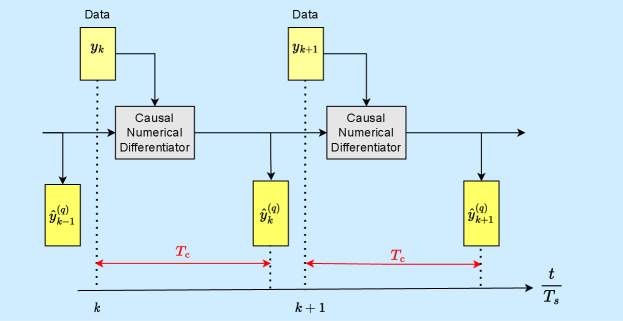
Several noteworthy differences exist among BD, SG, and HGO. First, BD differentiation operates on adjacent pairs of data points, whereas SG differentiation operates on a moving window of data points. Consequently, SG differentiation is potentially more accurate than BD differentiation. Because of the time needed for computation, all numerical differentiation entails an unavoidable delay in the availability of the estimated derivative. In addition, BD differentiation and HGO differentiation do not require future data to estimate the derivative, thus they are causal algorithms. On the other hand, SG differentiation requires future data, and thus it is noncausal. For causal differentiation, the delay is step due to computation; for noncausal differentiation, . Assuming Figure 1 illustrates the case . Note that for BD and HGO, whereas for SG with window size
To quantify the accuracy of each numerical differentiation algorithm, for all , we define the relative root-mean-square error (RMSE) of the estimate of the th derivative as
| (22) |
Note that numerator of (22) accounts for the effect of the delay For real-time implementation, the relevant error metric depends on the difference between the true current derivative and the currently available estimate of the past derivative, as can be seen in the numerator of (22). When the derivative estimates are exact, (22) determines an RMSE value that can be viewed as the delay floor for the th derivative, that is, the error due solely to the fact that a noncausal differentiation algorithm must be implemented with a suitable delay. Note that the delay floor depends on and is typically positive.
The true values of are the sampled values of in the absence of sensor noise. Of course, the true values of are unknown in practice and thus cannot be used as an online error criterion. However, these values are used in (22), which is computable in simulation for comparing the accuracy of the numerical differentiation algorithms.
To compare the various baseline algorithms presented in Section 2, we consider numerical differentiation of the continuous-time signal , where is time in seconds. The signal is sampled with sample time sec. The measurements are assumed to be corrupted by noise, and thus the noisy sampled signal is given by , where is standard (zero-mean, unit-variance, Gaussian) white noise. The value of is chosen to set the desired signal-to-noise ratio (SNR).
For single differentiation with SG, let and . For single differentiation with HGO, let HGO/1 denote HGO with , , , and , and let HGO/2 denote HGO/1 with replaced by . Figure 2 shows the relative RMSE of the estimate of the first derivative for SNR ranging from dB to dB, where steps.
For double differentiation with SG, let and . For double differentiation with HGO, let HGO/1 denote HGO with , , , , and , and let HGO/2 denote HGO/1 with replaced by . Figure 3 shows the relative RMSE of the estimate of the second derivative for SNR ranging from dB to dB, where steps. The delay floors in Figures 2 and 3 are determined by computing the RMSE between the true value and the -step-delayed true value .
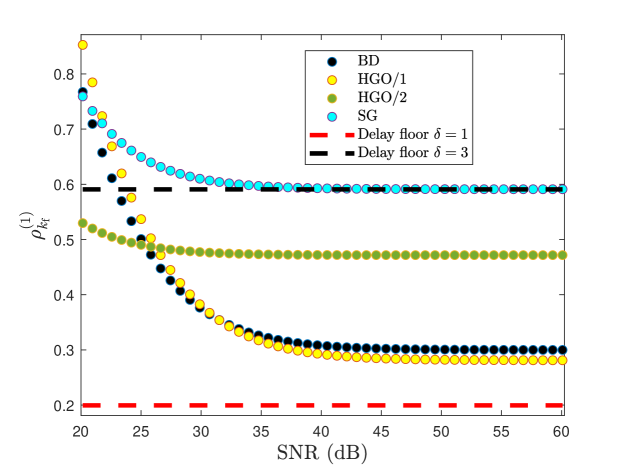
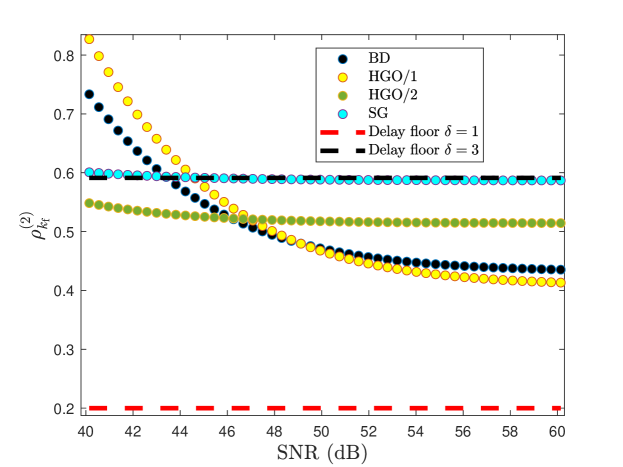
The comparison between HGO/1 and HGO/2 in Figure 2 and 3 shows that the performance of HGO differentiation depends on the noise level, and thus tuning is needed to achieve the best possible performance. When the noise level is unknown, however, this tuning is not possible. Hence, we now consider a differentiation technique that adapts to the actual noise characteristics.
4 Adaptive Input Estimation
This section discusses adaptive input estimation (AIE), which is a specialization of retrospective cost input estimation (RCIE) derived in Ansari \BBA Bernstein (\APACyear2019). This section explains how AIE specializes RCIE to the problem of causal numerical differentiation.
Consider the linear discrete-time system
| (23) | ||||
| (24) |
where is the step, is the state, , is standard white noise, and is the sensor noise. The matrices , , , and are assumed to be known. Define the sensor-noise covariance . The goal of AIE is to estimate and .
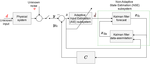
AIE consists of three subsystems, namely, the Kalman filter forecast subsystem, the input-estimation subsystem, and the Kalman filter data-assimilation subsystem. First, consider the Kalman filter forecast step
| (25) | |||
| (26) | |||
| (27) |
where is the estimate of , is the data-assimilation state, is the forecast state, is the residual, and .
Next, to obtain , the input-estimation subsystem of order is given by the exactly proper dynamics
| (28) |
where and . AIE minimizes by using recursive least squares (RLS) to update and as shown below. The subsystem (28) can be reformulated as
| (29) |
where the regressor matrix is defined by
| (30) |
the coefficient vector is defined by
| (31) |
and . In terms of the backward-shift operator , (28) can be written as
| (32) |
where
| (33) | ||||
| (34) | ||||
| (35) |
To update the coefficient vector we define the filtered signals
| (36) |
where, for all ,
| (37) |
| (41) |
and , where is the Kalman filter gain given by (47) below. Furthermore, define the retrospective variable
| (42) |
where the coefficient vector denotes a variable for optimization, and define the retrospective cost function
| (43) |
where , and is positive definite. Then, for all , the unique global minimizer of (43) is given by the RLS update as shown in Islam \BBA Bernstein (\APACyear2019)
| (44) | ||||
| (45) |
where
Using the updated coefficient vector given by (45), the estimated input at step is given by replacing by in (29). We choose and thus Implementation of AIE requires that the user specify the orders and as well as the weightings and These parameters are specified for each example in the paper.
4.1 State Estimation
The forecast variable given by (25) is used to obtain the estimate of given by the Kalman filter data-assimilation step
| (46) |
where the state estimator gain , the data-assimilation error covariance and the forecast error covariance are given by
| (47) | ||||
| (48) | ||||
| (49) |
, and
4.2 Application of AIE to Numerical Differentiation
5 Adaptive Input and State Estimation
In practice, and may be unknown in (49) and (47). To address this problem, three versions of AIE are presented. In each version, and may or may not be adapted. These versions are summarized in Table 1.
| Adaptation | Adaptation | |
| AIE/NSE | No | No |
| AIE/SSE | Yes | No |
| AIE/ASE | Yes | Yes |
To adapt and , at each step we define the computable performance metric
| (51) |
where is the sample variance of over given by
| (52) | ||||
| (53) |
and is the variance of the residual given by the Kalman filter, that is,
| (54) |
Note that (51) is the difference between the theoretical and empirical variances of , which provides an indirect measure of the accuracy of and
5.1 AIE with Non-adaptive State Estimation (AIE/NSE)
In AIE/NSE, is fixed at a user-chosen value, and is assumed to be known and fixed at its true value. AIE/NSE is thus a specialization of AIE with in (49) and in (47), where is the true value of the sensor-noise covariance. A block diagram of AIE/NSE is shown in Figure 4.
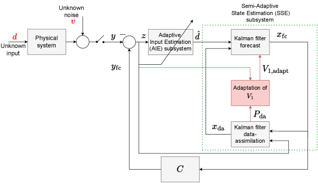
5.2 AIE with Semi-adaptive State Estimation (AIE/SSE)
In AIE/SSE, is adapted, and is assumed to be known and fixed at its true value. Let denote the adapted value of . AIE/SSE is thus a specialization of AIE with in (49) and in (47). In particular, such that
| (55) |
where and A block diagram of AIE/SSE is shown in Figure 5.
5.3 AIE with Adaptive State Estimation (AIE/ASE)
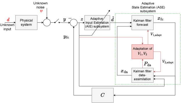
In AIE/ASE, both and are adapted. Let denote the adapted value of . AIE/ASE is thus a specialization of AIE with in (49) and in (47). In particular, and such that
| (56) |
where and Defining
| (57) |
and using (54), (51) can be rewritten as
| (58) |
We construct a set of positive values of by enumerating as
| (59) |
and are then chosen based on following two cases.
Case 1. If is not empty, then
| (60) | ||||
| (61) |
where
| (62) |
and . For all of the examples in this paper, we set and omit the argument of
Case 2. If is empty, then
| (63) | ||||
| (64) |
A block diagram of AIE/ASE is shown in Figure 6. AIE/ASE is summarized by Algorithm 1.
6 Numerical Differentiation of Two-Tone Harmonic Signal
In this section, a numerical example is given to compare the accuracy of the numerical differentiation algorithms discussed in the previous sections. We consider a two-tone harmonic signal, and we compare the accuracy (relative RMSE) of BD, HGO/1, SG, AIE/NSE, AIE/SSE, and AIE/ASE. For single and double differentiation, the parameters for HGO/1 and SG are given in Section 3.
Example 6.1.
Differentiation of a two-tone harmonic signal
Consider the continuous-time signal , where is time in seconds. The signal is sampled with sample time sec. The measurements are assumed to be corrupted by noise, and thus the noisy sampled signal is given by , where is standard white noise.
Single Differentiation. For AIE/NSE, let , , and for SNR dB. For AIE/SSE, the parameters are the same as those of AIE/NSE, except that is adapted, where and in Section 5.2. Similarly, for AIE/ASE, the parameters are the same as those of AIE/SSE except that is adapted as in Section 5.3.
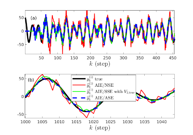
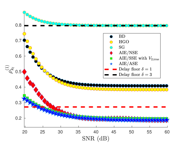
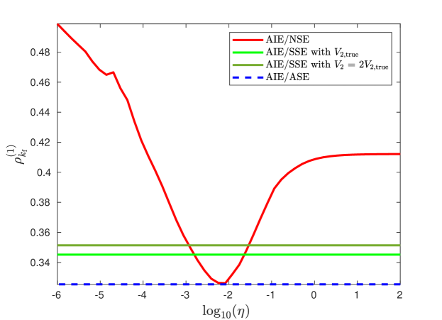
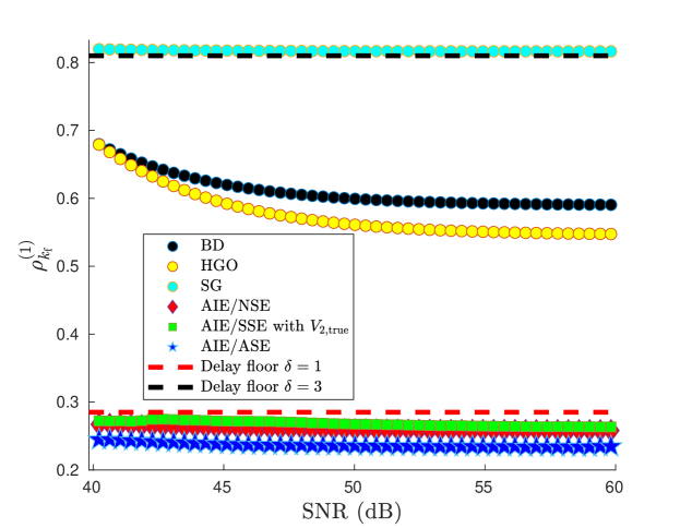
Figure 7 compares the true first derivative with the estimates obtained from AIE/NSE, AIE/SSE, and AIE/ASE. Figure 8 shows that AIE/ASE has the best accuracy over the range of SNR. Figure 9 shows that the accuracy of AIE/ASE is close to the best accuracy of AIE/NSE.
Double Differentiation. For AIE/NSE, let , , and for SNR dB. For AIE/SSE, the parameters are the same as those of AIE/NSE, except that is adapted, where and in Section 5.2. Similarly, for AIE/ASE, the parameters are the same as those of AIE/SSE except that is adapted as in Section 5.3.
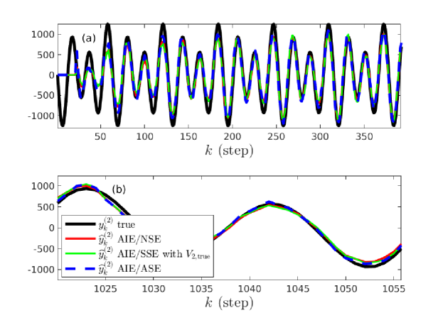
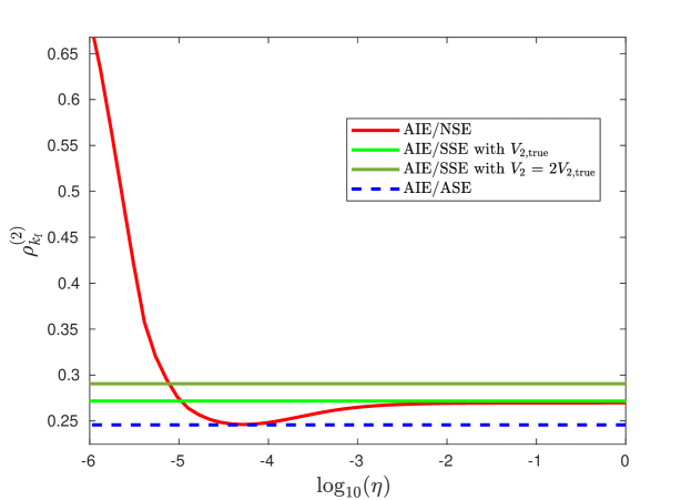
Figure 10 compares the true second derivative with the estimates obtained from AIE/NSE, AIE/SSE with , and AIE/ASE. Figure 11 shows that AIE/ASE has the best accuracy over the range of SNR. Figure 12 shows that the accuracy of AIE/ASE is close to the best accuracy of AIE/NSE.
7 Application to Ground-Vehicle Kinematics
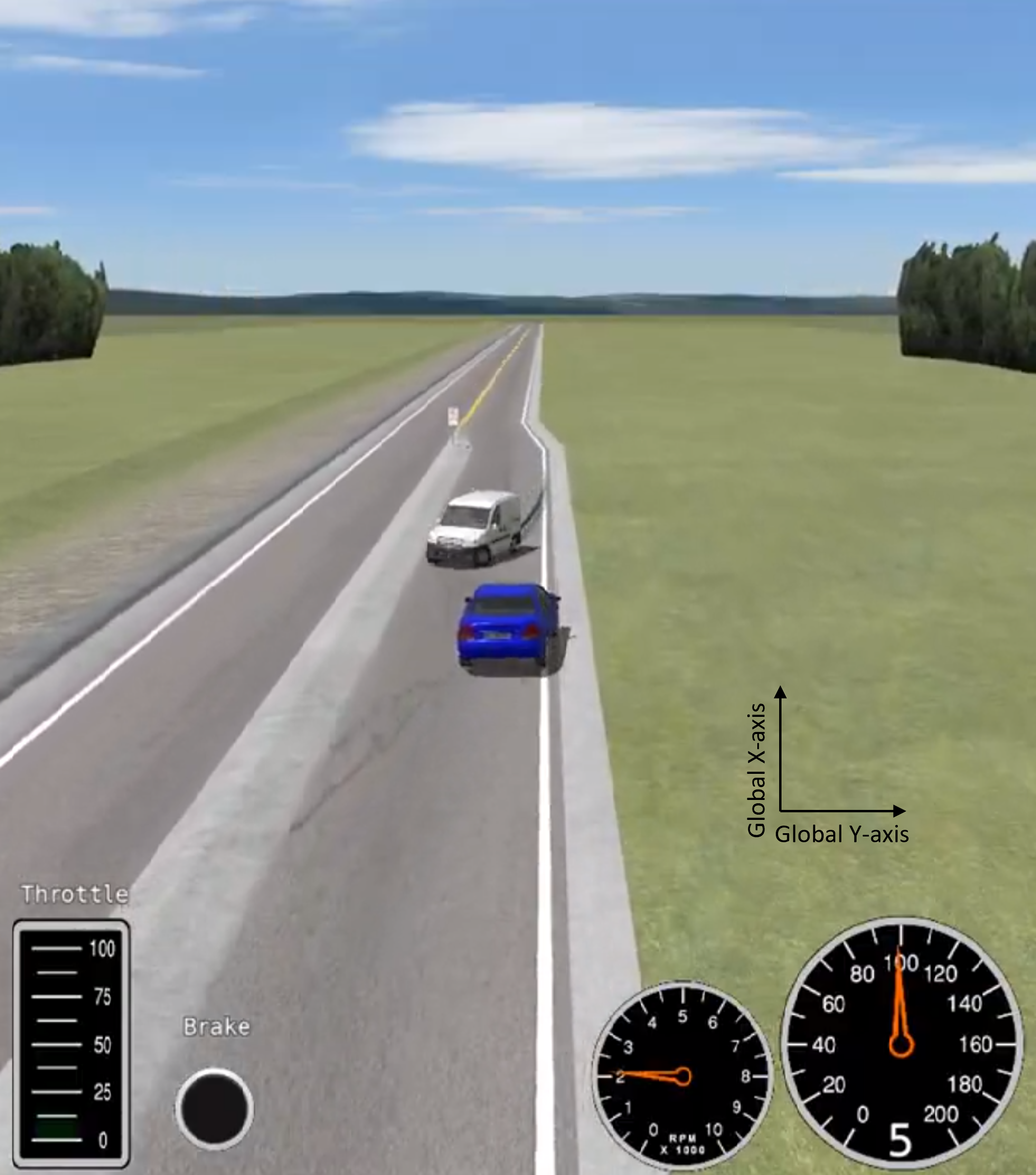
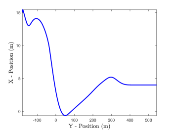
In this section, CarSim is used to simulate a scenario in which an oncoming vehicle (the white van in Figure 13) slides over to the opposing lane. The host vehicle (the blue van) performs an evasive maneuver to avoid a collision. Relative position data along the global y-axis (shown in Figure 13) is differentiated to estimate the relative velocity and acceleration along the same axis. Figure 14 shows the relative position trajectory of the vehicles on the - plane
Example 7.1.
Differentiation of CarSim position data.
Discrete-time position data generated by CarSim is corrupted with discrete-time, zero-mean, Gaussian white noise whose variance is chosen to vary the SNR.
Single Differentiation
For AIE/NSE, let , , , and for SNR dB. For AIE/SSE, the parameters are the same as those of AIE/NSE, except that is adapted, where and in Section 5.2. Similarly, for AIE/ASE, the parameters are the same as those of AIE/SSE except that is adapted as in Section 5.3.
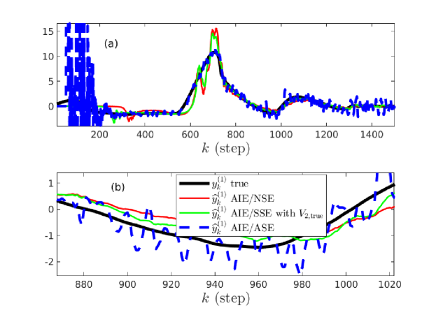
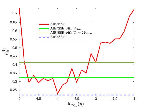
Figure 15 compares the true first derivative with the estimates obtained from AIE/NSE, AIE/SSE with , and AIE/ASE. Figure 16 shows that the accuracy of AIE/ASE is close to the best accuracy of AIE/NSE.
Double Differentiation
For AIE/NSE, Let , , and for SNR dB. For AIE/SSE, the parameters are the same as those of AIE/NSE, except that is adapted, where and in Section 5.2. Similarly, for AIE/ASE, the parameters are the same as those of AIE/SSE except that is adapted as in Section 5.3.
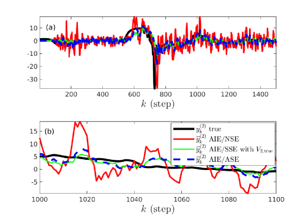
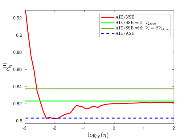
Figure 17 compares the true second derivative with the estimates obtained from AIE/NSE, AIE/SSE with , and AIE/ASE. Figure 18 shows that the accuracy of AIE/ASE is close to the best accuracy of AIE/NSE.
8 Conclusions
This paper presented the adaptive input and state estimation algorithm AIE/ASE for causal numerical differentiation. AIE/ASE uses the Kalman-filter residual to adapt the input-estimation subsystem and an empirical estimate of the estimation error to adapt the input-estimation and sensor-noise covariances. For dual-tone harmonic signals with various levels of sensor noise, the accuracy of AIE/ASE was compared to several conventional numerical differentiation methods. Finally, AIE/ASE was applied to simulated vehicle position data generated by CarSim.
Future work will focus on the following extensions. The minimization of (56) was performed by using a gridding procedure; more efficient optimization is possible. Next, the choice of in (62) was found to provide good accuracy in all examples considered; however, further investigation is needed to refine this choice. Furthermore, it is of interest to compare the accuracy of AIE/ASE to the adaptive sliding mode differentiator in Alwi \BBA Edwards (\APACyear2013). Finally, in practice, the spectrum of the measured signal and sensor noise may change abruptly. In these cases, it may be advantageous to replace the RLS update (44), (45) with RLS that uses variable-rate forgetting in Bruce \BOthers. (\APACyear2020); Mohseni \BBA Bernstein (\APACyear2022).
Acknowledgments
This research was supported by Ford and NSF grant CMMI 2031333.
Disclosure statement
No potential conflict of interest was reported by the author(s).
References
- Ahn \BOthers. (\APACyear2006) \APACinsertmetastarramm2{APACrefauthors}Ahn, S., Choi, U\BPBIJ.\BCBL \BBA Ramm, A\BPBIG. \APACrefYearMonthDay2006. \BBOQ\APACrefatitleA Scheme for Stable Numerical Differentiation A Scheme for Stable Numerical Differentiation.\BBCQ \APACjournalVolNumPagesJ. Comp. Appl. Math.1862325–334. \PrintBackRefs\CurrentBib
- Alenezi \BOthers. (\APACyear2021) \APACinsertmetastarZakTAC2021{APACrefauthors}Alenezi, B., Zhang, M., Hui, S.\BCBL \BBA Zak, S\BPBIH. \APACrefYearMonthDay2021. \BBOQ\APACrefatitleSimultaneous Estimation of the State, Unknown Input, and Output Disturbance in Discrete-Time Linear Systems Simultaneous Estimation of the State, Unknown Input, and Output Disturbance in Discrete-Time Linear Systems.\BBCQ \APACjournalVolNumPagesIEEE Trans. Autom. Contr.66126115–6122. \PrintBackRefs\CurrentBib
- Almagbile \BOthers. (\APACyear2010) \APACinsertmetastarAlmagbile2010{APACrefauthors}Almagbile, A., Wang, J.\BCBL \BBA Ding, W. \APACrefYearMonthDay20106. \BBOQ\APACrefatitleEvaluating the Performances of Adaptive Kalman Filter Methods in GPS/INS Integration Evaluating the Performances of Adaptive Kalman Filter Methods in GPS/INS Integration.\BBCQ \APACjournalVolNumPagesJ. Global Pos. Sys.933-40. \PrintBackRefs\CurrentBib
- Alwi \BBA Edwards (\APACyear2013) \APACinsertmetastaralwi_adap_sliding_mode_2012{APACrefauthors}Alwi, H.\BCBT \BBA Edwards, C. \APACrefYearMonthDay2013. \BBOQ\APACrefatitleAn Adaptive Sliding Mode Differentiator for Actuator Oscillatory Failure Case Reconstruction An Adaptive Sliding Mode Differentiator for Actuator Oscillatory Failure Case Reconstruction.\BBCQ \APACjournalVolNumPagesAutomatica492642-651. \PrintBackRefs\CurrentBib
- Ansari \BBA Bernstein (\APACyear2019) \APACinsertmetastaransari_input_2019{APACrefauthors}Ansari, A.\BCBT \BBA Bernstein, D\BPBIS. \APACrefYearMonthDay2019. \BBOQ\APACrefatitleInput Estimation for Nonminimum-Phase Systems With Application to Acceleration Estimation for a Maneuvering Vehicle Input Estimation for Nonminimum-Phase Systems With Application to Acceleration Estimation for a Maneuvering Vehicle.\BBCQ \APACjournalVolNumPagesIEEE Trans. Contr. Sys. Tech.2741596–1607. \PrintBackRefs\CurrentBib
- Astrom \BBA Hagglund (\APACyear2006) \APACinsertmetastarPIDastrom{APACrefauthors}Astrom, K.\BCBT \BBA Hagglund, T. \APACrefYear2006. \APACrefbtitleAdvanced PID Control Advanced PID Control. \APACaddressPublisherISA. \PrintBackRefs\CurrentBib
- Bogler (\APACyear1987) \APACinsertmetastarbogler_1987{APACrefauthors}Bogler, P. \APACrefYearMonthDay1987. \BBOQ\APACrefatitleTracking a Maneuvering Target Using Input Estimation Tracking a Maneuvering Target Using Input Estimation.\BBCQ \APACjournalVolNumPagesIEEE Trans. Aero. Elec. Sys.AES-233298-310. \PrintBackRefs\CurrentBib
- Bruce \BOthers. (\APACyear2020) \APACinsertmetastaradamVRF{APACrefauthors}Bruce, A., Goel, A.\BCBL \BBA Bernstein, D\BPBIS. \APACrefYearMonthDay2020. \BBOQ\APACrefatitleConvergence and Consistency of Recursive Least Squares with Variable-Rate Forgetting Convergence and Consistency of Recursive Least Squares with Variable-Rate Forgetting.\BBCQ \APACjournalVolNumPagesAutomatica119109052. \PrintBackRefs\CurrentBib
- Cullum (\APACyear1971) \APACinsertmetastarcullum{APACrefauthors}Cullum, J. \APACrefYearMonthDay1971. \BBOQ\APACrefatitleNumerical Differentiation and Regularization Numerical Differentiation and Regularization.\BBCQ \APACjournalVolNumPagesSIAM J. Num. Anal.8254–265. \PrintBackRefs\CurrentBib
- Dabroom \BBA Khalil (\APACyear1999) \APACinsertmetastardabroom_discrete-time_1999{APACrefauthors}Dabroom, A\BPBIM.\BCBT \BBA Khalil, H\BPBIK. \APACrefYearMonthDay1999. \BBOQ\APACrefatitleDiscrete-time Implementation of High-Gain Observers for Numerical Differentiation Discrete-time Implementation of High-Gain Observers for Numerical Differentiation.\BBCQ \APACjournalVolNumPagesInt. J. Contr.72171523–1537. \PrintBackRefs\CurrentBib
- Davis \BBA Rabinowitz (\APACyear1984) \APACinsertmetastardavis{APACrefauthors}Davis, P\BPBIJ.\BCBT \BBA Rabinowitz, P. \APACrefYear1984. \APACrefbtitleMethods of Numerical Integration Methods of Numerical Integration (\PrintOrdinalsecond \BEd). \APACaddressPublisherDover. \PrintBackRefs\CurrentBib
- Fang \BOthers. (\APACyear2011) \APACinsertmetastarfang2011stable{APACrefauthors}Fang, H., Shi, Y.\BCBL \BBA Yi, J. \APACrefYearMonthDay2011. \BBOQ\APACrefatitleOn Stable Simultaneous Input and State Estimation for Discrete-Time Linear Systems On Stable Simultaneous Input and State Estimation for Discrete-Time Linear Systems.\BBCQ \APACjournalVolNumPagesInt. J. Adapt. Contr. Sig. Proc.258671–686. \PrintBackRefs\CurrentBib
- Farrell (\APACyear2008) \APACinsertmetastarfarrellAN{APACrefauthors}Farrell, J\BPBIA. \APACrefYear2008. \APACrefbtitleAided Navigation: GPS with High Rate Sensors Aided navigation: Gps with high rate sensors. \APACaddressPublisherMcGraw-Hill. \PrintBackRefs\CurrentBib
- Gillijns \BBA De Moor (\APACyear2007) \APACinsertmetastargillijns2007unbiased{APACrefauthors}Gillijns, S.\BCBT \BBA De Moor, B. \APACrefYearMonthDay2007. \BBOQ\APACrefatitleUnbiased Minimum-Variance Input and State Estimation for Linear Discrete-Time Systems Unbiased Minimum-Variance Input and State Estimation for Linear Discrete-Time Systems.\BBCQ \APACjournalVolNumPagesAutomatica431111–116. \PrintBackRefs\CurrentBib
- Grewel \BOthers. (\APACyear2020) \APACinsertmetastargrewal{APACrefauthors}Grewel, M\BPBIS., Andrews, A\BPBIP.\BCBL \BBA Bartone, C\BPBIG. \APACrefYear2020. \APACrefbtitleGlobal Navigation Satellite Systems, Inertial Navigation, and Integration Global navigation satellite systems, inertial navigation, and integration (\PrintOrdinalfourth \BEd). \APACaddressPublisherWiley. \PrintBackRefs\CurrentBib
- Haimovich \BOthers. (\APACyear2022) \APACinsertmetastarhaimovich2022{APACrefauthors}Haimovich, H., Seeber, R., Aldana-López, R.\BCBL \BBA Gómez-Gutiérrez, D. \APACrefYearMonthDay2022. \BBOQ\APACrefatitleDifferentiator for Noisy Sampled Signals With Best Worst-Case Accuracy Differentiator for Noisy Sampled Signals With Best Worst-Case Accuracy.\BBCQ \APACjournalVolNumPagesIEEE Contr. Sys. Lett.6938-943. \PrintBackRefs\CurrentBib
- Hamming (\APACyear1973) \APACinsertmetastarhamming{APACrefauthors}Hamming, R\BPBIW. \APACrefYear1973. \APACrefbtitleNumerical Methods of Scientists and Engineers Numerical Methods of Scientists and Engineers (\PrintOrdinalsecond \BEd). \APACaddressPublisherDover. \PrintBackRefs\CurrentBib
- Hide \BOthers. (\APACyear2003) \APACinsertmetastarHide2003{APACrefauthors}Hide, C., Moore, T.\BCBL \BBA Smith, M. \APACrefYearMonthDay20031. \BBOQ\APACrefatitleAdaptive Kalman Filtering for Low-Cost INS/GPS Adaptive Kalman Filtering for Low-Cost INS/GPS.\BBCQ \APACjournalVolNumPagesJ. Nav.56143-152. \PrintBackRefs\CurrentBib
- H. Khaloozadeh (\APACyear2009) \APACinsertmetastarkarsaz_2009{APACrefauthors}H. Khaloozadeh, A\BPBIK. \APACrefYearMonthDay2009. \BBOQ\APACrefatitleModified Input Estimation Technique for Tracking Manoeuvring Targets Modified Input Estimation Technique for Tracking Manoeuvring Targets.\BBCQ \APACjournalVolNumPagesIET Radar Sonar Nav.330-41. \PrintBackRefs\CurrentBib
- Hsieh (\APACyear2017) \APACinsertmetastarhsieh2017unbiased{APACrefauthors}Hsieh, C\BHBIS. \APACrefYearMonthDay2017. \BBOQ\APACrefatitleUnbiased Minimum-Variance Input and State Estimation for Systems with Unknown Inputs: A System Reformation Approach Unbiased Minimum-Variance Input and State Estimation for Systems with Unknown Inputs: A System Reformation Approach.\BBCQ \APACjournalVolNumPagesAutomatica84236–240. \PrintBackRefs\CurrentBib
- Islam \BBA Bernstein (\APACyear2019) \APACinsertmetastarislam2019recursive{APACrefauthors}Islam, S\BPBIA\BPBIU.\BCBT \BBA Bernstein, D\BPBIS. \APACrefYearMonthDay2019. \BBOQ\APACrefatitleRecursive Least Squares for Real-Time Implementation Recursive least squares for real-time implementation.\BBCQ \APACjournalVolNumPagesIEEE Contr. Sys. Mag.39382–85. \PrintBackRefs\CurrentBib
- Jauberteau \BBA Jauberteau (\APACyear2009) \APACinsertmetastarJauberteau2009{APACrefauthors}Jauberteau, F.\BCBT \BBA Jauberteau, J. \APACrefYearMonthDay2009. \BBOQ\APACrefatitleNumerical Differentiation with Noisy Signal Numerical Differentiation with Noisy Signal.\BBCQ \APACjournalVolNumPagesAppl. Math. Comp.2152283–2297. \PrintBackRefs\CurrentBib
- Jia \BOthers. (\APACyear2008) \APACinsertmetastarjia_2008{APACrefauthors}Jia, Z., Balasuriya, A.\BCBL \BBA Challa, S. \APACrefYearMonthDay2008. \BBOQ\APACrefatitleAutonomous Vehicles Navigation with Visual Target Tracking: Technical Approaches Autonomous Vehicles Navigation with Visual Target Tracking: Technical Approaches.\BBCQ \APACjournalVolNumPagesAlgorithms12153–182. \PrintBackRefs\CurrentBib
- Kalata (\APACyear1984) \APACinsertmetastarkalata_1984{APACrefauthors}Kalata, P\BPBIR. \APACrefYearMonthDay1984. \BBOQ\APACrefatitleThe Tracking Index: A Generalized Parameter for - and -- Target Trackers The Tracking Index: A Generalized Parameter for - and -- Target Trackers.\BBCQ \APACjournalVolNumPagesIEEE Trans. Aero. Elec. Sys.AES-202174-182. \PrintBackRefs\CurrentBib
- Knowles \BBA Renka (\APACyear2014) \APACinsertmetastarknowles_methods{APACrefauthors}Knowles, I.\BCBT \BBA Renka, R\BPBIJ. \APACrefYearMonthDay2014. \BBOQ\APACrefatitleMethods for Numerical Differentiation of Noisy Data Methods for Numerical Differentiation of Noisy Data.\BBCQ \APACjournalVolNumPagesElectron. J. Diff. Eqn.21235–246. \PrintBackRefs\CurrentBib
- Lee \BBA Tahk (\APACyear1999) \APACinsertmetastarlee_1999{APACrefauthors}Lee, H.\BCBT \BBA Tahk, M\BHBIJ. \APACrefYearMonthDay1999. \BBOQ\APACrefatitleGeneralized Input-Estimation Technique for Tracking Maneuvering Targets Generalized Input-Estimation Technique for Tracking Maneuvering Targets.\BBCQ \APACjournalVolNumPagesIEEE Trans. Aero. Elec. Sys.3541388-1402. \PrintBackRefs\CurrentBib
- Levant (\APACyear2003) \APACinsertmetastararie2003slidemode{APACrefauthors}Levant, A. \APACrefYearMonthDay2003. \BBOQ\APACrefatitleHigher-Order Sliding Modes, Differentiation and Output-Feedback Control Higher-Order Sliding Modes, Differentiation and Output-Feedback Control.\BBCQ \APACjournalVolNumPagesInt. J. Contr.769-10924–941. \PrintBackRefs\CurrentBib
- Listmann \BBA Zhao (\APACyear2013) \APACinsertmetastarzhao2013{APACrefauthors}Listmann, K\BPBID.\BCBT \BBA Zhao, Z. \APACrefYearMonthDay2013. \BBOQ\APACrefatitleA Comparison of Methods for Higher-Order Numerical Differentiation A Comparison of Methods for Higher-Order Numerical Differentiation.\BBCQ \BIn \APACrefbtitleProc. Eur. Contr. Conf. Proc. eur. contr. conf. (\BPGS 3676–3681). \PrintBackRefs\CurrentBib
- López-Caamal \BBA Moreno (\APACyear2019) \APACinsertmetastarlopez-caamal_generalised_2019{APACrefauthors}López-Caamal, F.\BCBT \BBA Moreno, J\BPBIA. \APACrefYearMonthDay2019. \BBOQ\APACrefatitleGeneralised Multivariable Supertwisting Algorithm Generalised Multivariable Supertwisting Algorithm.\BBCQ \APACjournalVolNumPagesInt. J. Robust Nonlinear Contr.293634–660. \PrintBackRefs\CurrentBib
- Mboup \BOthers. (\APACyear2009) \APACinsertmetastarmboupnumeralg{APACrefauthors}Mboup, M., Join, C.\BCBL \BBA Fliess, M. \APACrefYearMonthDay2009. \BBOQ\APACrefatitleNumerical Differentiation with Annihilators in Noisy Environment Numerical Differentiation with Annihilators in Noisy Environment.\BBCQ \APACjournalVolNumPagesNum. Algor.50439–467. \PrintBackRefs\CurrentBib
- Mehra (\APACyear1972) \APACinsertmetastarMehra1972{APACrefauthors}Mehra, R\BPBIK. \APACrefYearMonthDay1972. \BBOQ\APACrefatitleApproaches to Adaptive Filtering Approaches to Adaptive Filtering.\BBCQ \APACjournalVolNumPagesIEEE Trans. Autom. Contr.17693-698. \PrintBackRefs\CurrentBib
- Moghe \BOthers. (\APACyear2019) \APACinsertmetastarmoghe2019adaptivekfLTI{APACrefauthors}Moghe, R., Zanetti, R.\BCBL \BBA Akella, M\BPBIR. \APACrefYearMonthDay2019. \BBOQ\APACrefatitleAdaptive Kalman Filter for Detectable Linear Time-Invariant Systems Adaptive Kalman Filter for Detectable Linear Time-Invariant Systems.\BBCQ \APACjournalVolNumPagesJ. Guid. Contr. Dyn.42102197–2205. \PrintBackRefs\CurrentBib
- Mohamed \BBA Schwarz (\APACyear1999) \APACinsertmetastarMohamed1999{APACrefauthors}Mohamed, A\BPBIH.\BCBT \BBA Schwarz, K\BPBIP. \APACrefYearMonthDay1999. \BBOQ\APACrefatitleAdaptive Kalman Filtering for INS/GPS Adaptive Kalman Filtering for INS/GPS.\BBCQ \APACjournalVolNumPagesJ. Geodesy193-203. \PrintBackRefs\CurrentBib
- Mohseni \BBA Bernstein (\APACyear2022) \APACinsertmetastarnimaFtest{APACrefauthors}Mohseni, N.\BCBT \BBA Bernstein, D\BPBIS. \APACrefYearMonthDay2022. \BBOQ\APACrefatitleRecursive Least Squares with Variable-Rate Forgetting Based on the F-Test Recursive Least Squares with Variable-Rate Forgetting Based on the F-Test.\BBCQ \BIn \APACrefbtitleProc. Amer. Contr. Conf. Proc. amer. contr. conf. (\BPGS 3937–3942). \PrintBackRefs\CurrentBib
- Mojallizadeh \BOthers. (\APACyear2021) \APACinsertmetastarmojallizadeh2021{APACrefauthors}Mojallizadeh, M\BPBIR., Brogliato, B.\BCBL \BBA Acary, V. \APACrefYearMonthDay2021. \BBOQ\APACrefatitleDiscrete-Time Differentiators: Design and Comparative Analysis Discrete-Time Differentiators: Design and Comparative Analysis.\BBCQ \APACjournalVolNumPagesInt. J. Robust Nonlinear Contr.31167679–7723. \PrintBackRefs\CurrentBib
- Mook \BBA Junkins (\APACyear1988) \APACinsertmetastarjunkins1988minimum{APACrefauthors}Mook, D\BPBIJ.\BCBT \BBA Junkins, J\BPBIL. \APACrefYearMonthDay1988. \BBOQ\APACrefatitleMinimum Model Error Estimation for Poorly Modeled Dynamic Systems Minimum Model Error Estimation for Poorly Modeled Dynamic Systems.\BBCQ \APACjournalVolNumPagesJ. Guid. Contr. Dyn.113256–261. \PrintBackRefs\CurrentBib
- Naderi \BBA Khorasani (\APACyear2019) \APACinsertmetastarnaderi2019unbiased{APACrefauthors}Naderi, E.\BCBT \BBA Khorasani, K. \APACrefYearMonthDay2019. \BBOQ\APACrefatitleUnbiased Inversion-Based Fault Estimation of Systems with Non-Minimum Phase Fault-to-Output Dynamics Unbiased Inversion-Based Fault Estimation of Systems with Non-Minimum Phase Fault-to-Output Dynamics.\BBCQ \APACjournalVolNumPagesIET Contr. Theory Appl.13111629–1638. \PrintBackRefs\CurrentBib
- Nieuwstadt \BOthers. (\APACyear1998) \APACinsertmetastarNieuwstadt1998{APACrefauthors}Nieuwstadt, M\BPBIV., Rathinam, M.\BCBL \BBA Murray, R\BPBIM. \APACrefYearMonthDay1998. \BBOQ\APACrefatitleDifferential Flatness and Absolute Equivalence of Nonlinear Control Systems Differential flatness and absolute equivalence of nonlinear control systems.\BBCQ \APACjournalVolNumPagesSIAM J. Contr. Optim.3641225–1239. \PrintBackRefs\CurrentBib
- Orjuela \BOthers. (\APACyear2009) \APACinsertmetastarorjuela2009simultaneous{APACrefauthors}Orjuela, R., Marx, B., Ragot, J.\BCBL \BBA Maquin, D. \APACrefYearMonthDay2009. \BBOQ\APACrefatitleOn the Simultaneous State and Unknown Input Estimation of Complex Systems via a Multiple Model Strategy On the Simultaneous State and Unknown Input Estimation of Complex Systems via a Multiple Model Strategy.\BBCQ \APACjournalVolNumPagesIET Contr. Theory Appl.37877–890. \PrintBackRefs\CurrentBib
- Rana \BOthers. (\APACyear2020) \APACinsertmetastarrana_2020{APACrefauthors}Rana, M\BPBIM., Halim, N., Rahamna, M\BPBIM.\BCBL \BBA Abdelhadi, A. \APACrefYearMonthDay2020. \BBOQ\APACrefatitlePosition and Velocity Estimations of 2D-Moving Object Using Kalman Filter: Literature Review Position and Velocity Estimations of 2D-Moving Object Using Kalman Filter: Literature Review.\BBCQ \BIn \APACrefbtitleProc. Int. Conf. Adv. Comm. Tech. Proc. int. conf. adv. comm. tech. (\BPG 541-544). \PrintBackRefs\CurrentBib
- Reichhartinger \BBA Spurgeon (\APACyear2018) \APACinsertmetastarreichhartinger_arbitrary-order_2018{APACrefauthors}Reichhartinger, M.\BCBT \BBA Spurgeon, S. \APACrefYearMonthDay2018. \BBOQ\APACrefatitleAn Arbitrary-Order Differentiator Design Paradigm with Adaptive Gains An Arbitrary-Order Differentiator Design Paradigm with Adaptive Gains.\BBCQ \APACjournalVolNumPagesInt. J. Contr.9192028–2042. \PrintBackRefs\CurrentBib
- Savitzky \BBA Golay (\APACyear1964) \APACinsertmetastarsavitzky1964smoothing{APACrefauthors}Savitzky, A.\BCBT \BBA Golay, M\BPBIJ. \APACrefYearMonthDay1964. \BBOQ\APACrefatitleSmoothing and Differentiation of Data by Simplified Least Squares Procedures Smoothing and Differentiation of Data by Simplified Least Squares Procedures.\BBCQ \APACjournalVolNumPagesAnal. Chemistry3681627–1639. \PrintBackRefs\CurrentBib
- Schafer (\APACyear2011) \APACinsertmetastarSG_lecture_notes_Schafer{APACrefauthors}Schafer, R\BPBIW. \APACrefYearMonthDay2011. \BBOQ\APACrefatitleWhat is a Savitzky-Golay Filter? What is a Savitzky-Golay Filter?\BBCQ \APACjournalVolNumPagesIEEE Sig. Proc. Mag.284111-117. \PrintBackRefs\CurrentBib
- Shi \BOthers. (\APACyear2009) \APACinsertmetastarshiadapukf2009{APACrefauthors}Shi, Y., Han, C.\BCBL \BBA Liang, Y. \APACrefYearMonthDay2009. \BBOQ\APACrefatitleAdaptive UKF for Target Tracking with Unknown Process Noise Statistics Adaptive UKF for Target Tracking with Unknown Process Noise Statistics.\BBCQ \BIn \APACrefbtitleProc. Int. Conf. Inf. Fusion Proc. int. conf. inf. fusion (\BPGS 1815–1820). \PrintBackRefs\CurrentBib
- Staggs (\APACyear2005) \APACinsertmetastarSG_staggs{APACrefauthors}Staggs, J\BPBIE\BPBIJ. \APACrefYearMonthDay2005. \BBOQ\APACrefatitleSavitzky–Golay Smoothing and Numerical Differentiation of Cone Calorimeter Mass Data Savitzky–Golay Smoothing and Numerical Differentiation of Cone Calorimeter Mass Data.\BBCQ \APACjournalVolNumPagesFire Safety J.406493-505. \PrintBackRefs\CurrentBib
- Stickel (\APACyear2010) \APACinsertmetastarStickel2010{APACrefauthors}Stickel, J. \APACrefYearMonthDay2010. \BBOQ\APACrefatitleData Smoothing and Numerical Differentiation by a Regularization Method Data Smoothing and Numerical Differentiation by a Regularization Method.\BBCQ \APACjournalVolNumPagesComp. Chem. Eng.34467–475. \PrintBackRefs\CurrentBib
- Van Breugel \BOthers. (\APACyear2020) \APACinsertmetastarKutz2020{APACrefauthors}Van Breugel, F., Kutz, J\BPBIN.\BCBL \BBA Brunton, B\BPBIW. \APACrefYearMonthDay2020. \BBOQ\APACrefatitleNumerical Differentiation of Noisy Data: A Unifying Multi-Objective Optimization Framework Numerical Differentiation of Noisy Data: A Unifying Multi-Objective Optimization Framework.\BBCQ \APACjournalVolNumPagesIEEE Access8196865–196877. \PrintBackRefs\CurrentBib
- Verma \BOthers. (\APACyear2022) \APACinsertmetastarshashankACC2022{APACrefauthors}Verma, S., Sanjeevini, S., Sumer, E\BPBID., Girard, A.\BCBL \BBA Bernstein, D\BPBIS. \APACrefYearMonthDay2022. \BBOQ\APACrefatitleOn the Accuracy of Numerical Differentiation Using High-Gain Observers and Adaptive Input Estimation On the Accuracy of Numerical Differentiation Using High-Gain Observers and Adaptive Input Estimation.\BBCQ \BIn \APACrefbtitleProc. Amer. Contr. Conf. Proc. amer. contr. conf. (\BPG 4068-4073). \PrintBackRefs\CurrentBib
- Vilanova \BBA Visioli (\APACyear2012) \APACinsertmetastarPID2012{APACrefauthors}Vilanova, R.\BCBT \BBA Visioli, A. \APACrefYear2012. \APACrefbtitlePID Control in the Third Millennium: Lessons Learned and New Approaches PID Control in the Third Millennium: Lessons Learned and New Approaches. \APACaddressPublisherSpringer. \PrintBackRefs\CurrentBib
- Yaesh \BBA Shaked (\APACyear2008) \APACinsertmetastarYaesh2008SimplifiedAE{APACrefauthors}Yaesh, I.\BCBT \BBA Shaked, U. \APACrefYearMonthDay2008. \BBOQ\APACrefatitleSimplified Adaptive Estimation Simplified Adaptive Estimation.\BBCQ \APACjournalVolNumPagesSys. Contr. Lett.5749–55. \PrintBackRefs\CurrentBib
- Yong \BOthers. (\APACyear2016) \APACinsertmetastaryong2016unified{APACrefauthors}Yong, S\BPBIZ., Zhu, M.\BCBL \BBA Frazzoli, E. \APACrefYearMonthDay2016. \BBOQ\APACrefatitleA Unified Filter for Simultaneous Input and State Estimation of Linear Discrete-Time Stochastic Systems A Unified Filter for Simultaneous Input and State Estimation of Linear Discrete-Time Stochastic Systems.\BBCQ \APACjournalVolNumPagesAutomatica63321–329. \PrintBackRefs\CurrentBib
- Zhang \BOthers. (\APACyear2020) \APACinsertmetastarzhangadapKF2020{APACrefauthors}Zhang, L., Sidoti, D., Bienkowski, A., Pattipati, K\BPBIR., Bar-Shalom, Y.\BCBL \BBA Kleinman, D\BPBIL. \APACrefYearMonthDay2020. \BBOQ\APACrefatitleOn the Identification of Noise Covariances and Adaptive Kalman Filtering: A New Look at a 50 Year-Old Problem On the Identification of Noise Covariances and Adaptive Kalman Filtering: A New Look at a 50 Year-Old Problem.\BBCQ \APACjournalVolNumPagesIEEE Access859362–59388. \PrintBackRefs\CurrentBib