Real-time Motion Planning for autonomous vehicles in dynamic environments

Mohammad Dehghani Tezerjani Computer Science and Engineering
University of North Texas
Texas, USA
[email protected] Dominic Carrillo Computer Science and Engineering
University of North Texas
Texas, USA
[email protected] Deyuan Qu {@IEEEauthorhalign} Sudip Dhakal Computer Science and Engineering
University of North Texas
Texas, USA
[email protected] Computer Science and Engineering
University of North Texas
Texas, USA
[email protected] Amir Mirzaeinia Computer Science and Engineering
University of North Texas
Texas, USA
[email protected] Qing Yang Computer Science and Engineering
University of North Texas
Texas, USA
[email protected]

Abstract

Recent advancements in self-driving car technologies have enabled them to navigate autonomously through various environments. However, one of the critical challenges in autonomous vehicle operation is trajectory planning, especially in dynamic environments with moving obstacles. This research aims to tackle this challenge by proposing a robust algorithm tailored for autonomous cars operating in dynamic environments with moving obstacles. The algorithm introduces two main innovations. Firstly, it defines path density by adjusting the number of waypoints along the trajectory, optimizing their distribution for accuracy in curved areas and reducing computational complexity in straight sections. Secondly, it integrates hierarchical motion planning algorithms, combining global planning with an enhanced $A^{*}$ graph-based method and local planning using the time elastic band algorithm with moving obstacle detection considering different motion models. The proposed algorithm is adaptable for different vehicle types and mobile robots, making it versatile for real-world applications. Simulation results demonstrate its effectiveness across various conditions, promising safer and more efficient navigation for autonomous vehicles in dynamic environments. These modifications significantly improve trajectory planning capabilities, addressing a crucial aspect of autonomous vehicle technology.

Index Terms:

Autonomous Vehicles, Dynamic obstacles, Obstacle avoidance, Global planning, Local planning, Timed elastic band, trajectory density

I Introduction

Today, the advancement of autonomous vehicle technology holds immense promise, offering significant benefits such as heightened safety, doubled efficiency, and increased accessibility, poised to revolutionize transportation systems. A critical aspect of autonomous vehicle development lies in creating a trajectory from the origin to the destination in the streets and places full of cars and pedestrians, which underscores the importance of high safety to prevent fatal accidents and damages[1]. According to the report of NHTSA, in 2021, 42,939 people died due to road accidents. This number was 39007 in 2020 and 36355 in 2019, which shows the increase in the number of deaths in recent years[2]. Most of the fatal cra were caused by drivers’ carelessness and mistakes, and 31% of these accidents are drunk drivers and 10% are distracted drivers[3, 4]. Autonomous vehicles present a groundbreaking opportunity to reduce errors and save lives significantly. They also serve as essential tools for individuals facing physical or visual challenges that hinder private car use. Concurrently, statistical data indicates that 86% of the American workforce relies on private car transportation, spending an average of 25 minutes driving daily[5]. By adopting autonomous vehicles, people can make more efficient use of their time and reduce the likelihood of experiencing neurological disorders linked to driving. In autonomous driving, three primary components are pivotal: perception, decision-making, and control[6]. The decision-making phase, especially critical in car navigation, is dedicated to generating paths for autonomous vehicles. This task can be segmented into two facets: path planning without temporal constraints and trajectory planning considering time factors. Crafting a path with temporal data entails determining factors like the time needed to reach specific points and the consequent vehicle speed or acceleration. Such planning also necessitates considering vehicle dynamics, dynamic obstacles, and environmental alterations not initially factored into the original mapping process[7]. Achieving autonomous navigation in vehicles relies on accurately describing the environment through mapping, identifying obstacles within it, generating obstacle-free routes from the starting point to the destination, and subsequently adhering to these routes. However, a significant challenge lies in enabling vehicles to navigate through dynamic environments. While current obstacles in trajectory generation primarily revolve around intricate real-time calculations in dynamic settings, this study specifically focuses on real-time motion planning in environments where dynamic obstacles are present.Motion planning strategies can be categorized into four main groups: graph search-based algorithms, sampling-based algorithms, interpolation curve algorithms, and numerical optimization methods[6]. Graph-based algorithms and sampling-based algorithms are commonly employed for global planning purposes[8]. While sampling-based algorithms offer faster performance, they are often probabilistic in nature and may not yield consistent results across iterations. Consequently, this study adopts an enhanced A* graph-based algorithm for global planning. Moreover, recent advancements in the field have introduced several algorithms tailored for local planning to mitigate collisions with moving obstacles. These include the artificial potential field algorithm [9], the dynamic window approach [10], the elastic band algorithm [11], and the timed elastic band algorithm [12]. The well-established elastic band method [11] is a dynamic trajectory planning approach that adapts the path’s shape in real-time. Internal forces, predefined within the method, ensure path continuity, while external forces help navigate around obstacles. However, the traditional elastic band method lacks consideration for time-related data and dynamic constraints. Building upon this, a method introduced in [12] extends the classic elastic band approach to incorporate temporal information in two stages. Initially, discrete intermediate waypoints are strategically positioned away from obstacles, followed by employing a dynamic movement model to ensure path continuity. In [13], these two stages are integrated to streamline the process. In contrast to the previously mentioned method, alternative approaches such as those utilized in Autoware’s waypoint generation process extract waypoints from the 3D map created during mapping and store them in a file [14]. While this file acts as a guide for path tracking, it operates independently of real-time constraints, thus introducing its own drawbacks. Trajectory optimization tasks often entail extensive computational efforts, posing challenges in integrating planning components with control units. Consequently, researchers seek efficient solutions for trajectory optimization problems. The dynamic window algorithm, introduced in [10], samples circular trajectories within a search space constrained by permissible linear and rotational speed orders to generate motion. In [15, 16], spline paths are continually optimized considering dynamic constraints. Additionally, [12] proposes the time elastic band method, an enhancement of the elastic band method that incorporates time data to optimize trajectories while avoiding obstacles. This study further improves the time elastic band method, enabling dynamic adjustments to trajectory accuracy based on current conditions. Furthermore, it estimates the trajectories of moving obstacles in the environment using the Kalman filter [17]. A combination of local planning algorithms and a predefined global planner facilitates real-time planning for autonomous vehicles in dynamic environments. Initially, motion planning in dynamic environments is conducted without temporal information. As the vehicle progresses along this path, it identifies new obstacles and adjusts the path accordingly. Through a hierarchical approach that integrates planning algorithms, this research aims to design optimal trajectories that minimize travel time while avoiding both stationary and moving obstacles, while adhering to the vehicle’s non-holonomic constraints[12].

II Methodology

In this study, the global planning method employed is the $A^{*}$ algorithm, enhanced with a gradient descent optimizer. Initially, the $A^{*}$ algorithm is applied to assign values to all map grids using a function, effectively creating an analogous discrete potential field within the environment. Subsequently, the gradient descent method is utilized to extract a favourable path from the origin to the destination based on these values. For local planning tasks, the timed elastic band method is preferred due to its numerous advantages over alternative motion planning approaches.

II-A Proposed algorithm for global planning

The proposed approach for global planning in this research involves utilizing the $A^{*}$ algorithm to assess a portion of the map and employing a decreasing gradient optimizer to determine the path. The $A^{*}$ algorithm is adept at finding the shortest path based on the distance criterion from the goal, making it suitable for global planning in both structured and unstructured environments. Incorporating heuristic criteria in this method significantly reduces computational complexity. By employing this approach, higher-probability path segments within the map are prioritized, effectively creating a representation akin to a discrete potential field in the environment. Subsequently, the gradient descent method is employed to derive the shortest path from the starting point to the destination. The $A^{*}$ algorithm leverages heuristic criteria to streamline calculations, while the use of gradients facilitates the discovery of smoother paths, enhancing its comparative value over other planning methods.The implementation of the $A^{*}$ algorithm in this research is outlined in Algorithm 1.

II-B $A^{*}$ planner

In the global planning method applied to the generated map, as integrated within the $A^{*}$ algorithm, the procedure entails receiving the cost map coordinates corresponding to the starting and ending points, and subsequently deriving the path from the end point. Initially, the path finder initializes the path array by placing the destination point. It then examines the eight neighbouring cell, selecting the one with the lowest value as the subsequent waypoint along the path. This iterative process persists until the starting point is reached.

II-C Gradient descent method

In this study, the gradient descent method is employed for path finding. Gradient descent is an iterative mathematical optimization algorithm utilized to locate the minimum of a function. It involves taking steps proportional to the negative gradient (or estimated gradient) of the function at the current point. If steps in the positive gradient direction are taken, the algorithm approaches the maximum of the function, known as the incremental gradient process. Here, the function of interest is discrete and two-dimensional, derived as a map from the A* method. The following pseudocode outlines the process of estimating the gradient on this map and determining the path:

Algorithm 1 Pseudocode for the modified

A^{*}

Algorithm

1:Initialize the overall cost-map with the start and goal locations.

2:Form an array of ordered pairs, where the first component denotes the cell index and the second component represents the cell value.

3:Set the initial value of all map points (except the starting point, which is set to zero) to a large value.

4:Place the starting point with a value of zero in the first position of the queue.

5:while the queue is not empty do

6: Extract the cell with the highest value from the queue.

7: if the end point is reached then

8: Terminate the process.

9: end if

10: for all neighboring cells (left, right, top, bottom) do

11: if cell value is less than a predefined threshold then

12: Remove the cell from consideration.

13: end if

14: if cell is outside the map boundary then

15: Remove the cell from consideration.

16: end if

17: Calculate the new value for the cell.

18: Compute the Euclidean distance from the cell to the end point.

19: Store the cell index, its new value, and the sum of the new value.

20: end for

21:end while

Algorithm 2 Pseudocode for

A^{*}

Algorithm

1:Begin from the destination point.

2:Continue until reaching the starting point:

3:while not at starting point do

4: if each neighboring cell value =

POT\_HIGH^{*}

then

5: Move to the neighboring cell with the lowest value.

6: else

7: Compute the numerical approximation of the potential gradient.

8: if gradient is zero then

9: An error has occurred.

10: end if

11: Move half a cell in the direction of the negative gradient.

12: end if

13:end while

${}^{*}POT\_HIGH$ : A very high initial value

Due to the heuristic criterion employed in the $A^{*}$ algorithm, only the map regions, where the presence of a path is more probable, are valued. Consequently, a potential error arises at the border between the valued area and the non-valued area when using the decreasing gradient method. This issue is addressed by adding the fourth and fifth lines, thereby rectifying the error.

II-D Proposed algorithm for local planning

After establishing the global path from the origin to the destination, accounting for static obstacles, the next step involves local planning to fine-tune the final trajectory for the vehicle. In this research, the local trajectory is defined as a sequence of vehicle positions along with the corresponding time intervals. Each position is characterized by four parameters detailing the vehicle’s location and orientation.

II-E Setting the trajectory density

The proposal outlined in this article aims to enhance trajectory quality while mitigating computational burden by augmenting the number of waypoints in critical sections, such as bends or turns. This is achieved by integrating a dynamic term into the time intervals within the fastest time cost function, enabling trajectory accuracy adjustments along specific segments. The cost function for the fastest route is introduced as Eq. 1.

f_{k}=\sum_{k=1}^{n-1}\left(\Delta T_{k}\right)^{2}

(1)

By selecting this cost function and employing the Lagrange coefficient, the inclination is to establish uniform time intervals throughout the path. However, assigning specific coefficients to individual time intervals allows for customization of their durations. Thus, the revised cost function is as Eq.2.

f_{k}=\sum_{k=1}^{n-1}w_{k}\left(\Delta T_{k}\right)^{2}

(2)

The larger the $w_{k}$ weight is, the smaller its corresponding time interval $\Delta T_{k}$ will be, and as a result, the accuracy of the trajectory will increase. Since the turns and curves of the route are among its sensitive parts[18], in this research, the accuracy of the path has been increased in the turns and curves of the route, and in the parts where the car moves in a straight line, in order to reduce the computational burden, a smaller number of waypoints have been used. The Eq.3 is used to identify the path curves, which is obtained according to Fig.1.

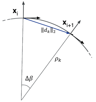
Refer to caption — Figure 1: Calculation of path curvature

\rho_{k}=\frac{\|d_{k}\|_{2}}{|2\sin\left(\frac{\Delta\beta_{k}}{2}\right)|}\quad(\text{since }\Delta\beta_{k}\ll 1)\quad\rho_{k}=\frac{\|d_{k}\|_{2}}{|\Delta\beta_{k}|}\geq\rho_{\text{min}}

(3)

This equation gives the radius of curvature of the path, the smaller the radius of curvature of the path, the more winding the path is. Therefore, according to the equation (4), the inverse value obtained from (3) is considered as the weight and is used for $w_{k}$ in the (5).

w_{k}=\frac{|\Delta\beta_{k}|}{\|d_{k}\|_{2}}

(4)

II-F Obstacle dynamics in local planning

For dynamic obstacle tracking, the position of the obstacle center is calculated every time the cost map is updated and given to the Kalman filter. A critical difference between motion planning for vehicles and mobile robots lies in the nature of the environment they navigate. In the case of vehicles, the planning environment encompasses fast moving vehicles, necessitating consideration of accelerated obstacle movement models. The Kalman filter emerges as a robust tool for providing scientific and engineering predictions regarding the future states of dynamic systems, particularly in scenarios where information about the system is imprecise. Notably, the Kalman filter boasts efficiency, requiring minimal memory as it relies solely on past state information. In this study, the Kalman filter leverages a constant acceleration motion model to estimate obstacle movement, thus yielding the following dynamic system equation.

\text{Pos\_est}=\text{Pos\_old}+V_{\text{rel}}\Delta t+\frac{1}{2}A_{\text{rel}}\Delta t^{2}

(5)

where, Pos_est is the estimated position of the obstacle, Pos_old is the previous position of the obstacle, $V_{\text{rel}}$ is the relative speed of the obstacle, $A_{\text{rel}}$ is the obstacle acceleration and $\Delta t$ represents the time interval between both iterations of the algorithm. To estimate the position, speed and acceleration of the obstacle, the relationship between these three parameters should be written in a standard way. The following equations contain these relationships.

	$\displaystyle\begin{bmatrix}\text{Pos}_{n+1}\\ \text{Vel}_{n+1}\end{bmatrix}$	$\displaystyle=\begin{bmatrix}1&t\\ 0&1\end{bmatrix}\begin{bmatrix}\text{Pos}_{n}\\ \text{Vel}_{n}\end{bmatrix}+\begin{bmatrix}\frac{t^{2}}{2}\\ t\end{bmatrix}\text{Acc}_{n}+\mathbf{w}_{n}$		(6)
	$\displaystyle Z_{n+1}$	$\displaystyle=\begin{bmatrix}1&0\end{bmatrix}\begin{bmatrix}\text{Pos}_{n+1}\\ \text{Vel}_{n+1}\end{bmatrix}+v_{n+1}$		(7)

$w_{n}$ is process noise and $v_{n}+1$ is observation noise, which are considered as white with zero mean. Considering that the above equation has an uncertain input of acceleration, the following equations can be used.

	$\displaystyle\begin{bmatrix}\text{Pos}_{n+1}\\ \text{Vel}_{n+1}\\ \text{Acc}_{n+1}\end{bmatrix}$	$\displaystyle=\begin{bmatrix}1&t&\frac{t^{2}}{2}\\ 0&1&t\\ 0&0&1\end{bmatrix}\begin{bmatrix}\text{Pos}_{n}\\ \text{Vel}_{n}\\ \text{Acc}_{n}\end{bmatrix}+\mathbf{w}_{n}$		(8)
	$\displaystyle Z_{n+1}$	$\displaystyle=\begin{bmatrix}1&t&\frac{t^{2}}{2}\end{bmatrix}\begin{bmatrix}\text{Pos}_{n}\\ \text{Vel}_{n}\\ \text{Acc}_{n}\end{bmatrix}+\mathbf{w}_{n}+v_{n+1}$		(9)

Table 1 shows the necessary definitions to use in Kalman equations.

TABLE I: System Augmented State

System state vector	$x_{\text{aug}}(n)=\begin{bmatrix}\text{Pos}_{n}\\ \text{Vel}_{n}\\ \text{Acc}_{n}\end{bmatrix}$
State transition model matrix	$F_{\text{aug}}(n)=\begin{bmatrix}1&t&\frac{t^{2}}{2}\\ 0&1&t\\ 0&0&1\end{bmatrix}$
Effect of noise level	$G_{\text{aug}}(n)=\begin{bmatrix}1\\ 1\\ 1\end{bmatrix}$
Observation model vector	$H_{\text{aug}}(n)=\begin{bmatrix}1&t&\frac{t^{2}}{2}\end{bmatrix}$
Observation noise	$v_{\text{aug}}(n)=w_{n}+v_{n+1}$
Process noise covariance	$Q_{\text{aug}}(n)=E\{w_{\text{aug}}(n)w_{\text{aug}}^{T}(n)\}=Q(n)$
Covariance of observation noise	$R_{\text{aug}}(n)=E\{v_{\text{aug}}(n)v_{\text{aug}}^{T}(n)\}$
	$=H(n)G(n)Q(n)G^{T}(n)H^{T}(n)+R(n)$
Correlation matrix of process noise	$T_{\text{aug}}(n)=E\{w_{\text{aug}}(n)v_{\text{aug}}^{T}(n)\}=Q(n)G^{T}(n)H^{T}(n)$

The following equations show the Kalman relations necessary to calculate the speed.

x\hat{\ }_{\text{aug}}(n|n-1)=F_{\text{aug}}(n)x\hat{\ }_{\text{aug}}(n-1|n-1)\\ \mathrm{\Sigma}_{\text{aug}}(n|n-1)=F_{\text{aug}}(n)\mathrm{\Sigma}_{\text{aug}}(n-1|n-1)F_{\text{aug}}^{T}(n)\\ +G_{\text{aug}}(n)Q_{\text{aug}}(n)G_{\text{aug}}^{T}(n)\\ y\hat{(n)}=Z_{\text{aug}}(n)-H_{\text{aug}}(n)x\hat{\ }_{\text{aug}}(n|n-1)\\ K_{\text{aug}}(n)=[\mathrm{\Sigma}_{\text{aug}}(n|n-1)H_{\text{aug}}^{T}(n)\\ +G_{\text{aug}}(n)T_{\text{aug}}(n)]R_{\text{aug}}^{-1}(n)\\ x\hat{\ }_{\text{aug}}(n|n)=x\hat{\ }_{\text{aug}}(n|n-1)+K_{\text{aug}}(n)y\hat{(n)}\\ \mathrm{\Sigma}_{\text{aug}}(n|n)=\mathrm{\Sigma}_{\text{aug}}(n|n-1)\\ -K_{\text{aug}}(n)H_{\text{aug}}(n)\mathrm{\Sigma}_{\text{aug}}(n|n-1)

(10)

In the above equations, $\hat{x}_{\text{aug}}$ is the estimated state vector, $\Sigma_{\text{aug}}$ is the covariance matrix of the estimation error, and $K_{\text{aug}}$ is the Kalman gain.

How to design the covariance noise process (Q matrix) is explained below. In practice, a lot of time is spent simulating and evaluating the collected data to choose the right value for Q. In general, the process model will be in the following form:

\dot{x}=Ax+Bu+w

(11)

where $w$ is the process noise.

The desired dynamic system is modeled using position, speed and acceleration. Now it is assumed that the acceleration, which is larger than the order, is constant in specific time intervals that are independent from each other and changes at the end of each interval. In other words, the acceleration jumps in each time interval and is modeled as below.

f(x)=Fx+\Gamma w

(12)

where $\Gamma$ is the system noise gain and $w$ is the desired continuous piece acceleration. The transfer matrix of the system is also defined as follows:

F=\begin{bmatrix}1&t&\frac{t^{2}}{2}\\ 0&1&t\\ 0&0&1\end{bmatrix}

(13)

In a period of time, the velocity changes as much as $w(t)\Delta t$ and the position changes as much as $w(t)\left(\Delta t\right)^{2}/2$ . As a result, it can be found that

\Gamma=\begin{bmatrix}\frac{\Delta t^{2}}{2}\\ \Delta t\\ 1\end{bmatrix}

(14)

Therefore, the covariance matrix of the system will be as follows.

Q=\mathbb{E}[\Gamma w(t)w(t)\Gamma^{T}]=\Gamma\sigma_{v}^{2}\Gamma^{T}

(15)

Q=\begin{bmatrix}\frac{\Delta t^{4}}{4}&\frac{\Delta t^{3}}{2}&\frac{\Delta t^{2}}{2}\\ \frac{\Delta t^{3}}{2}&\Delta t^{2}&\Delta t\\ \frac{\Delta t^{2}}{2}&\Delta t&1\end{bmatrix}

(16)

III Experiments

Fig.2 illustrates the scenario involving a parking lot, showcasing two planning methods: normal $A^{*}$ and gradient descent. Comparing the paths generated by these methods reveals that the gradient descent approach yields a notably smoother and optimal path compared to the conventional $A^{*}$ method. It’s worth noting that while the global planning may exhibit suboptimal outcomes, the local planner effectively mitigates many of its drawbacks, this means that the imperfections are okay and do not need special care when putting the plan into action. In designing the global planner, the paramount considerations include ensuring completeness, accuracy, and reducing computational complexity. Simulations validate that the proposed algorithm in this study satisfactorily fulfills these criteria, making it well-suited for global path planning.

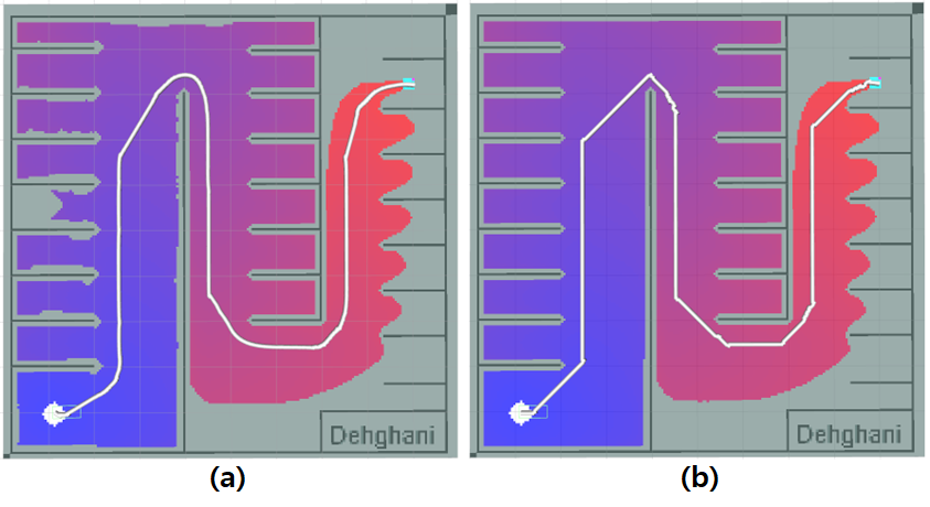
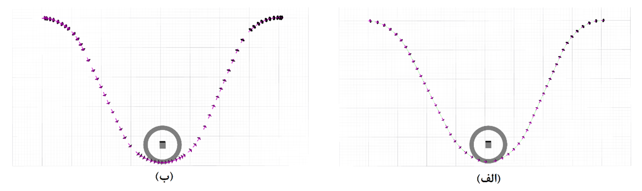
Fig.3 illustrates the impact of path density enhancement. Here, the origin is located at (-4, 0) and the destination at (+4, 0), while the obstacle has shifted from a position above the horizontal axis to (0, -4.5). Each arrow along the path indicates specific positions and directions for the car to traverse towards reaching the destination. Despite local optimization efforts and the path’s continuous shape alteration, without multipath optimization, the resulting path remains suboptimal. This scenario was conducted solely to introduce curvature into the path and evaluate improvements in this aspect. Higher curvature regions entail more waypoints, thus increasing path density accordingly.

To assess the effectiveness of the Kalman filter, various scenarios were examined involving moving obstacles with diverse velocities and accelerations. Their positions were calculated, and this data was subsequently fed into the Kalman filter to extract the motion model of the obstacle.

III-A First scenario: The obstacle moves at a constant speed in the vertical (y) direction

In this scenario, the moving obstacle is positioned ahead of the vehicle and travels along the y-axis (Fig.4(a)). The obstacle’s displacement is such that its linear velocity in the x-axis is zero, while its linear velocity in the y-axis changes completely randomly.

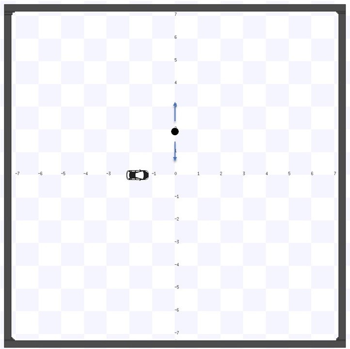
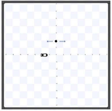
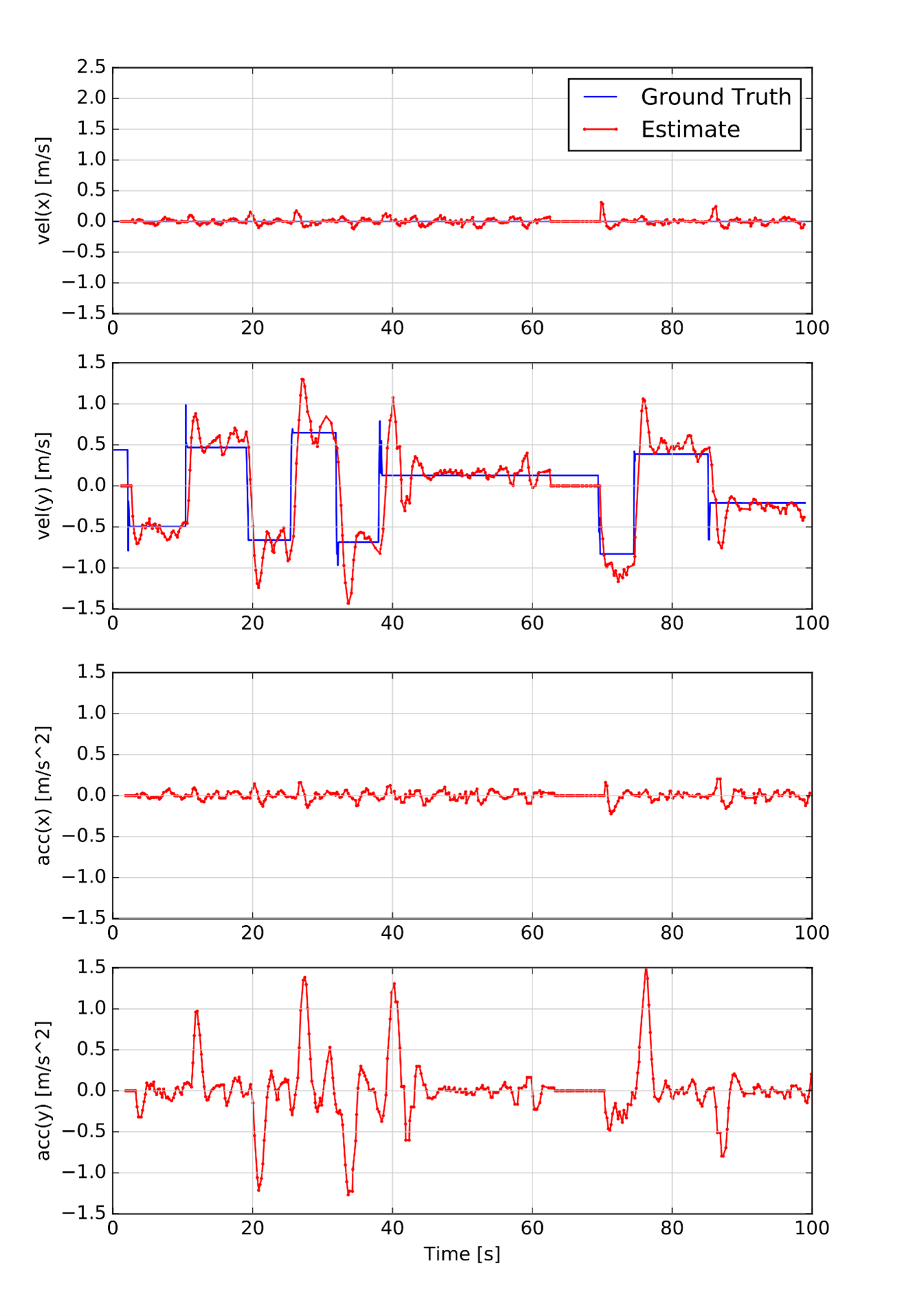
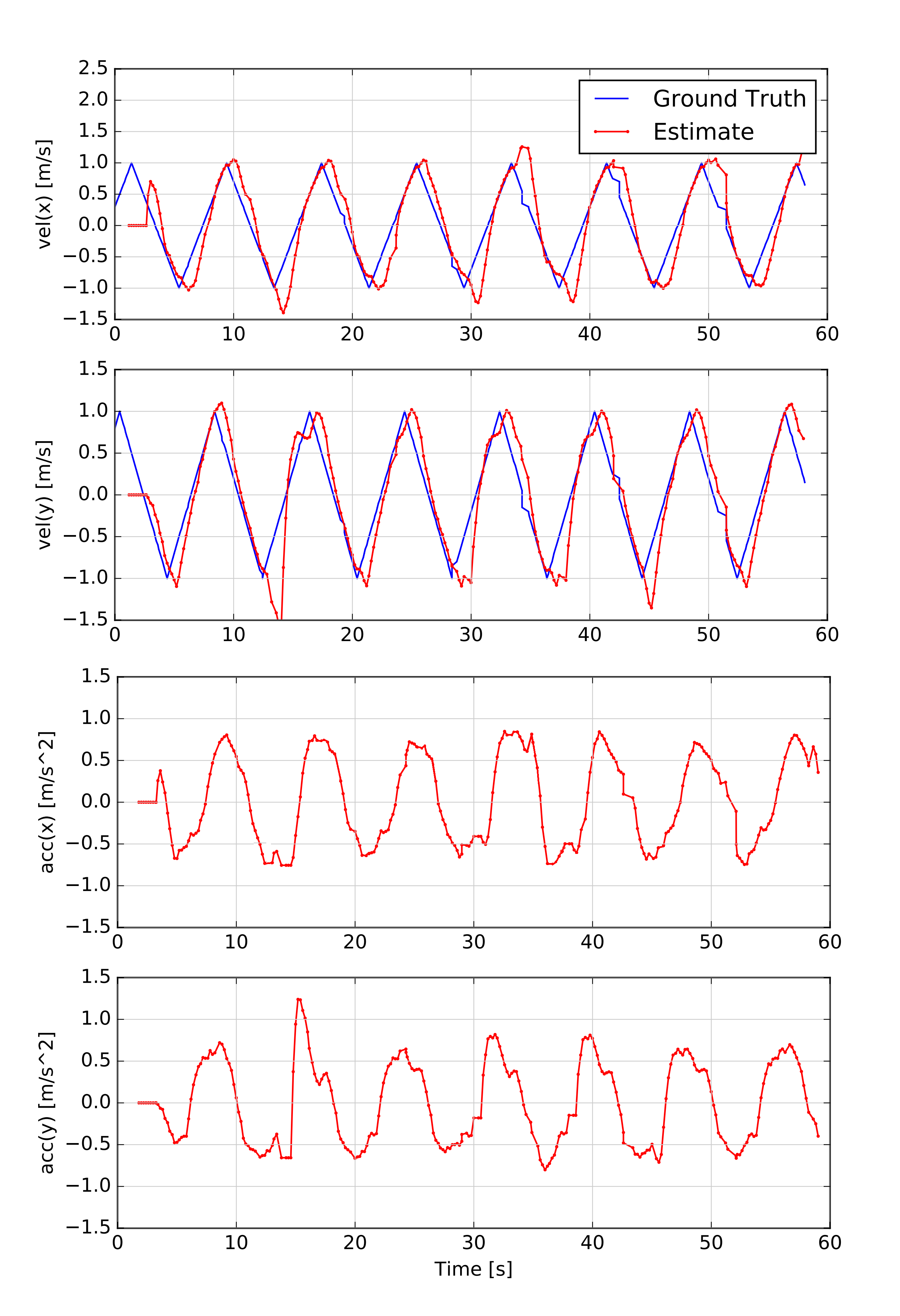
To confine the obstacle within the planning environment, its movement is constrained to a defined interval, with its direction changed upon reaching upper and lower limits. Despite large error in the perception phase and challenges in calculating the obstacle’s position, the Kalman filter adeptly estimates the speed and acceleration of the obstacle system.(Fig.4(d))

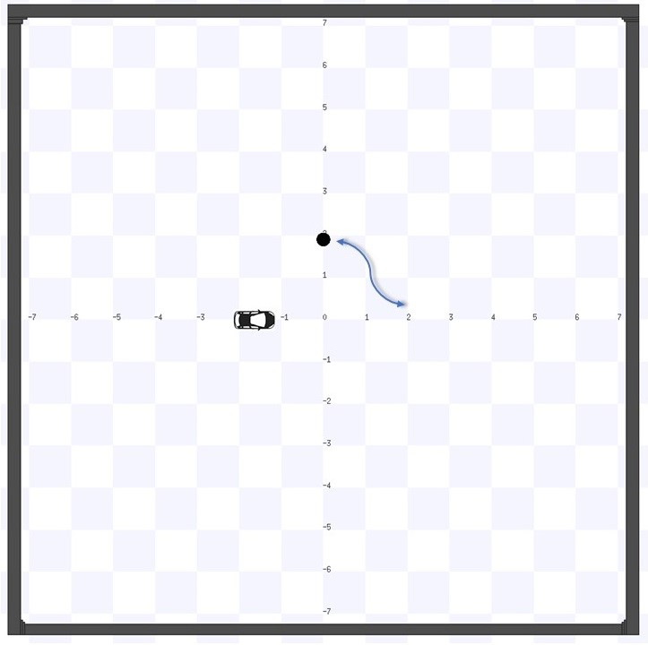
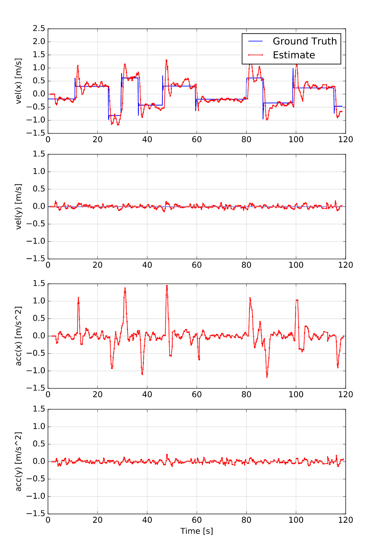
III-B Second scenario: The obstacle moves at a constant speed in the vertical (x) direction

In this scenario, the obstacle is positioned ahead of the vehicle and travels along the x-axis.(Fig.4(b)) Its displacement is designed so that its linear velocity in the y-direction remains zero while its linear velocity in the x-direction varies randomly. To ensure the obstacle remains within the routing environment, its movement is confined to a specific interval, and its direction is altered upon reaching the left and right boundaries. Despite significant error in calculating the obstacle’s position, the Kalman filter effectively estimates the speed and acceleration of the obstacle system.(Fig.4(e)) This scenario was tested to demonstrate the algorithm’s robustness to variations in the obstacle’s movement direction.

III-C Third scenario: The obstacle moves with a constant acceleration

To assess the Kalman filter’s performance in scenarios involving accelerated motion, a moving obstacle was subjected to constant acceleration within the environment. To limit the obstacle’s movement within the designated area, its linear velocities in the $x$ and $y$ directions were modulated using triangular functions. Depending on the frequency and amplitude of these functions, the trajectory of the obstacle varied. Despite the challenges in accurately calculating the obstacle’s position, the Kalman filter effectively estimated its speed and acceleration, highlighting its robustness even in the presence of significant error in the perception phase.(Fig.4(c)(f))

IV Motion planning in the presence of moving obstacles

IV-A First test: Static obstacles

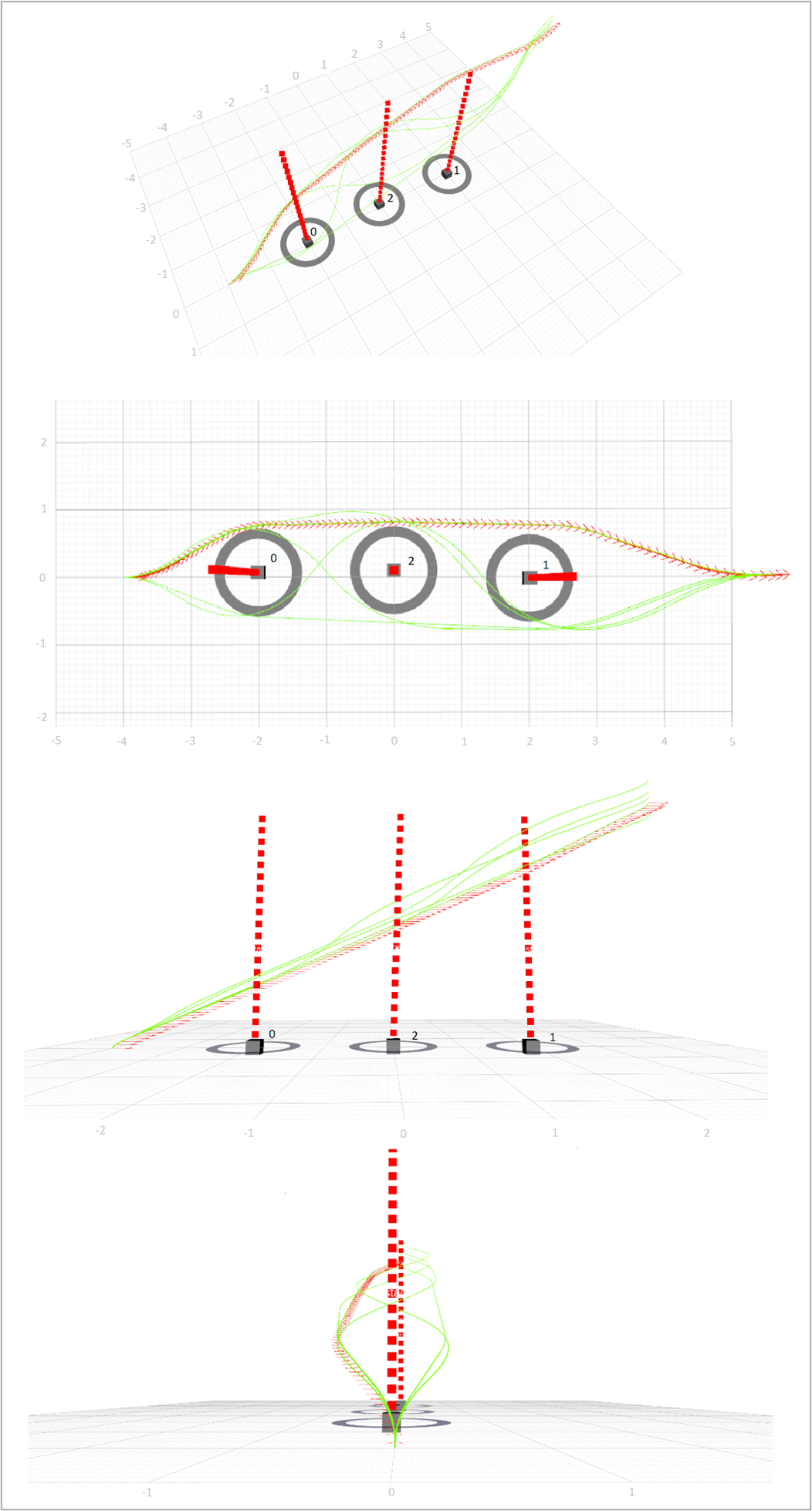
In order to test the performance of the algorithm, the initial values specified in Table II have been used.

TABLE II: Initial conditions for the first test

Description	Details
Initial position of the vehicle	$[-4,0]$
Destination location of the vehicle	$[4,0]$
	$0:[-2,0]$
Initial position of obstacles	$1:[2,0]$
	$2:[0,0]$
Dynamic conditions of obstacles	Completely static

The maximum number of homotopy classes is limited at 5 to control the computational workload. Consequently, 5 trajectories are simultaneously generated, and the one with the lowest cost is chosen. In the fig.5(a) red arrows denote the waypoints for the vehicle to traverse from the origin to the destination. The obstacles are considered as points and the circle around them indicates the safety margin. Obstacles can have any shape and be placed in any position. In order to show how the obstacles affect the path, it has been tried to place the obstacles at a point that has the greatest impact on the path. The final trajectory comprises 81 states, with an estimated time of arrival at 20.14 seconds. The average path computation time is 14.91milliseconds, which is considered efficient for a computer equipped with a dual-core processor running at 1.8 GHz.

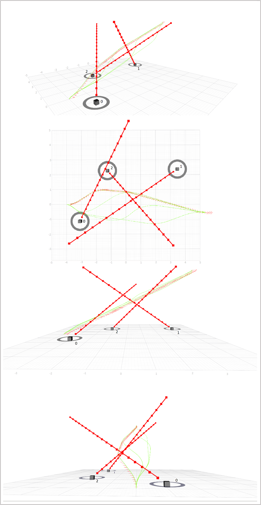
IV-B Second scenario: moving obstacles at a constant speed

In order to test the performance of the algorithm, the initial values specified in Table III have been used in this scenario.

TABLE III: Initial conditions for the Second test

Description	Details
Initial position of the vehicle	$[-4,0]$
Destination location of the vehicle	$[4,0]$
	$0:[-2,0]$
Initial position of obstacles	$1:[2,0]$
	$2:[0,0]$
	$0:[0.2,0.3]$
Initial speed of obstacles	$1:[-0.2,-0.3]$
	$2:[0.2,-0.2]$
Dynamic conditions of obstacles	Constant velocity

The maximum number of homotopy classes is set to four to avoid the increase in the computational cost. Therefore, four trajectories are designed simultaneously and the one that has a lower cost is selected. In the fig.5(b) the red arrows show the situations that the car must go through to go from the origin to the destination. The obstacles are simplified to points, with a surrounding circle denoting the safety margin. These obstacles are versatile, capable of assuming any shape and position. To demonstrate their influence on the path, obstacles are strategically positioned to show their maximum impact. The resulting route includes 75 states and the time to reach the destination will be 19.22 seconds. The average time required to calculate the path is 23.1 milliseconds, which is a good time for a computer with a dual-core processor with a frequency of 1.8 GHz.

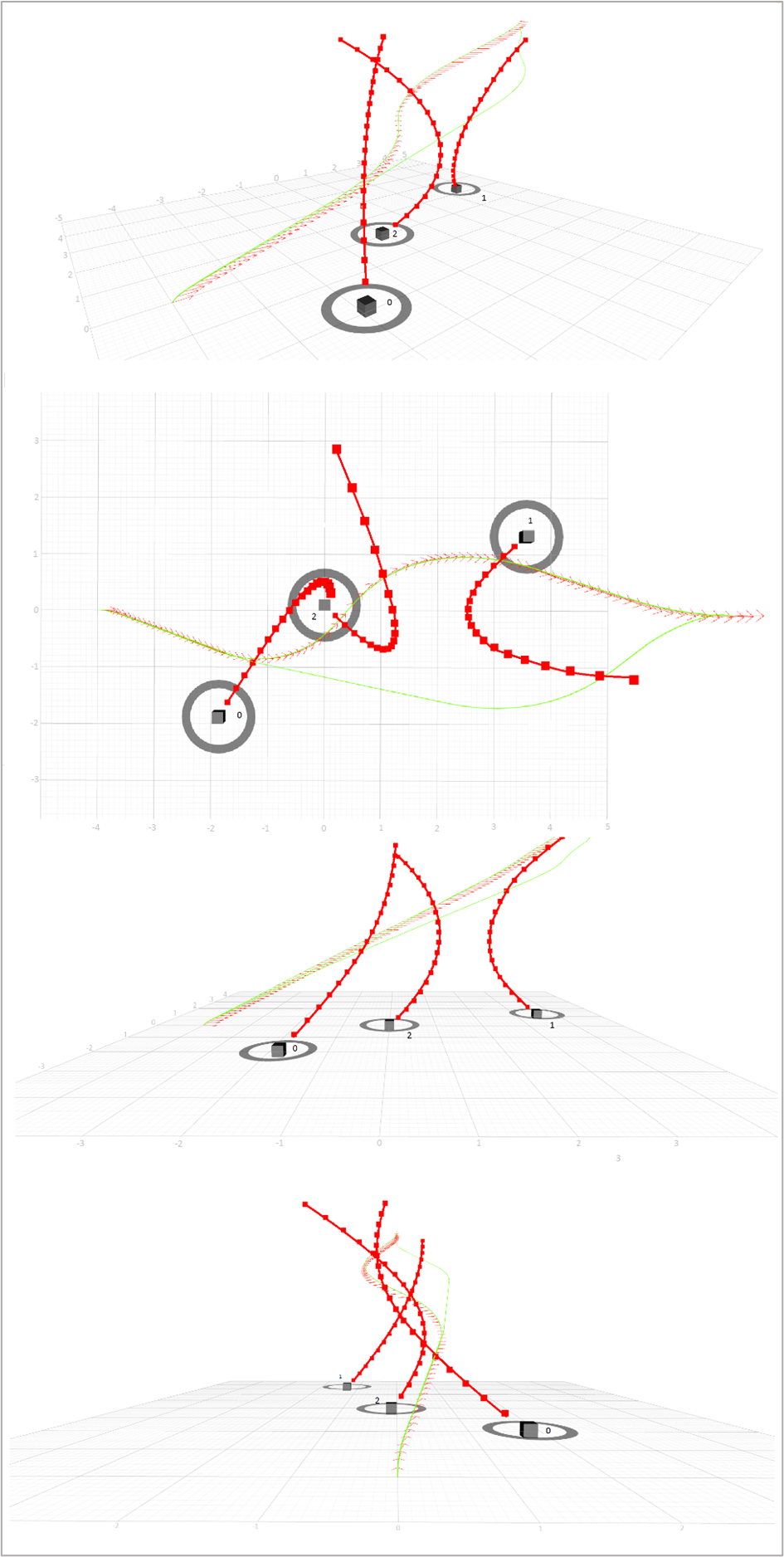
IV-C Third test: Accelerated moving obstacles

In order to test the performance of the algorithm, the initial values specified in Table IV have been used.

TABLE IV: Initial conditions for the Third test

Description	Details
Initial position of the vehicle	$[-4,0]$
Destination location of the vehicle	$[4,0]$
	$0:[-2,0]$
Initial position of obstacles	$1:[2,0]$
	$2:[0,0]$
	$0:[0.2,0.3]$
Initial speed of obstacles	$1:[-0.2,-0.3]$
	$2:[0.2,-0.2]$
	$0:[-0.01,-0.02]$
Initial speed of obstacles	$1:[0.03,0.01]$
	$2:[-0.02,0.03]$
Dynamic conditions of obstacles	Constant acceleration

The resulting route includes 85 states and the time to reach the destination will be 21.12 seconds. The average time required to calculate the route is 27.32 seconds, which is a good time for a computer with a dual-core processor with a frequency of 1.8 GHz. Fig.5(c) illustrates the scenario of accelerated obstacles.

V Conclusion

This research introduces the novel concept of ”Trajectory density” to assess the quality of generated paths by vehicle motion planning algorithms. By defining a new objective function and applying dynamic coefficients, this criterion is enhanced. Given that increasing the number of track conditions escalates computational load, it’s impractical to boost trajectory density throughout its entirety. Hence, the technique proposed in this study detects sensitive areas of the route, such as bends, and adjusts the density accordingly. Motion planning in the proposed method incorporates dynamics of moving obstacles. To identify obstacles and their locations, a new method is employed, amalgamating sensor data to produce a local cost-map. Computer vision methods are then utilized to differentiate between fixed and moving obstacles, with the latter’s location provided at a specific frequency enabling dynamic obstacle tracking. This information is integrated into the Kalman filter to estimate speed and acceleration, enabling extraction of obstacle dynamics.

References

Passmore et al. [2019] J. Passmore, Y. Yon, and B. Mikkelsen, “Progress in reducing road-traffic injuries in the who european region,” The Lancet Public Health, vol. 4, no. 6, pp. e272–e273, 2019. [Online]. Available: https://www.sciencedirect.com/science/article/pii/S246826671930074X
for Statistics and Analysis [2023] N. N. C. for Statistics and Analysis, “Summary of motor vehicle traffic crashes,” https://crashstats.nhtsa.dot.gov/Api/Public/ViewPublication/813515, 2023, [Accessed 01-03-2024].
Singh [2015] S. Singh, “Critical reasons for crashes investigated in the national motor vehicle crash causation survey,” Tech. Rep., 2015.
Singh [2018] ——, “Critical reasons for crashes investigated in the national motor vehicle crash causation survey,” Feb 2018. [Online]. Available: https://trid.trb.org/view/1507603
Gibson [2024] J. Gibson, “Commuting To Work in the US: Facts and Statistics — Bankrate — bankrate.com,” https://www.bankrate.com/insurance/car/commuting-facts-statistics/, 2024, [Accessed 02-03-2024].
González et al. [2015] D. González, J. Pérez, V. Milanés, and F. Nashashibi, “A review of motion planning techniques for automated vehicles,” IEEE Transactions on intelligent transportation systems, vol. 17, no. 4, pp. 1135–1145, 2015.
Kunchev et al. [2006] V. Kunchev, L. Jain, V. Ivancevic, and A. Finn, “Path planning and obstacle avoidance for autonomous mobile robots: A review,” in Knowledge-Based Intelligent Information and Engineering Systems: 10th International Conference, KES 2006, Bournemouth, UK, October 9-11, 2006. Proceedings, Part II 10. Springer, 2006, pp. 537–544.
Sanchez-Ibanez et al. [2021] J. R. Sanchez-Ibanez, C. J. Perez-del Pulgar, and A. García-Cerezo, “Path planning for autonomous mobile robots: A review,” Sensors, vol. 21, no. 23, p. 7898, 2021.
Khatib [1986] O. Khatib, “Real-time obstacle avoidance for manipulators and mobile robots,” The international journal of robotics research, vol. 5, no. 1, pp. 90–98, 1986.
Fox et al. [1997] D. Fox, W. Burgard, and S. Thrun, “The dynamic window approach to collision avoidance,” IEEE Robotics & Automation Magazine, vol. 4, no. 1, pp. 23–33, 1997.
Quinlan [1995] S. Quinlan, Real-time modification of collision-free paths. Stanford University, 1995.
Rösmann et al. [2012] C. Rösmann, W. Feiten, T. Wösch, F. Hoffmann, and T. Bertram, “Trajectory modification considering dynamic constraints of autonomous robots,” in ROBOTIK 2012; 7th German Conference on Robotics. VDE, 2012, pp. 1–6.
Kurniawati and Fraichard [2007] H. Kurniawati and T. Fraichard, “From path to trajectory deformation,” in 2007 IEEE/RSJ International Conference on Intelligent Robots and Systems. IEEE, 2007, pp. 159–164.
Dhakal et al. [2021] S. Dhakal, D. Qu, D. Carrillo, Q. Yang, and S. Fu, “Oasd: An open approach to self-driving vehicle,” in 2021 Fourth International Conference on Connected and Autonomous Driving (MetroCAD), 2021, pp. 54–61.
Lau et al. [2009] B. Lau, C. Sprunk, and W. Burgard, “Kinodynamic motion planning for mobile robots using splines,” in 2009 IEEE/RSJ International Conference on Intelligent Robots and Systems. IEEE, 2009, pp. 2427–2433.
Sprunk et al. [2011] C. Sprunk, B. Lau, P. Pfaffz, and W. Burgard, “Online generation of kinodynamic trajectories for non-circular omnidirectional robots,” in 2011 IEEE International Conference on Robotics and Automation. IEEE, 2011, pp. 72–77.
Welch et al. [1995] G. Welch, G. Bishop et al., “An introduction to the kalman filter,” 1995.
Li et al. [2022] B. Li, Y. Ouyang, L. Li, and Y. Zhang, “Autonomous driving on curvy roads without reliance on frenet frame: A cartesian-based trajectory planning method,” IEEE Transactions on Intelligent Transportation Systems, vol. 23, no. 9, pp. 15 729–15 741, 2022.