Real-time Impurity Solver Using Grassmann Time-Evolving Matrix Product Operators

The Hamiltonian for a general QIP can be written as

where $\hat{H}_{\rm imp}$ is the impurity Hamiltonian usually given by

Here $\hat{a}^{\dagger}$, $\hat{a}$ are the fermionic creation and annihilation operators. The subscripts $p,q,r,s$ represent the fermion flavors that contain both the spin and orbital indices. $\hat{H}_{\rm bath}$ is the bath Hamiltonian which can be written as

where $k$ denotes the momentum label, and $\varepsilon_{p,k}$ denotes corresponding energy. $\hat{H}_{\rm hyb}$ is the hybridization Hamiltonian between the impurity and bath. We will focus on linear coupling such that the bath can be integrated out using the Feynman-Vernon IF [59, 60, 61], which takes the following form:

with $V_{p,k}$ indicating the hybridization strength. For notational simplicity and as the general practice, we focus on flavor-independent $\hat{H}_{\rm bath}$ and $\hat{H}_{\rm hyb}$, such that we can write $\varepsilon_{p,k}=\varepsilon_{k}$ and $V_{p,k}=V_{k}$ for brevity.

Now we introduce several notations that will be used throughout this work. The separable impurity-bath initial state is denoted as

where $\hat{\rho}_{\mathrm{imp}}$ is some arbitrary impurity state and $\hat{\rho}_{\mathrm{bath}}^{{\rm eq}}\propto e^{-\beta\hat{H}_{\rm bath}}$ is the thermal equilibrium state of the bath at inverse temperature $\beta$. The thermal equilibrium state of the impurity plus bath at inverse temperature $\beta$ will be denoted as

The non-equilibrium retarded Green’s function will be denoted as (here $\Theta(t)$ is the Heaviside step function)

Here $G^{{\rm neq},>}_{p,q}(t,t^{\prime})$ and $G^{{\rm neq},<}_{p,q}(t,t^{\prime})$ denote the greater and lesser Green’s functions, respectively. They are defined as

where $\expectationvalue*{\cdots}_{\mathrm{neq}}=\Tr[\hat{\rho}_{\mathrm{tot}}^{\mathrm{neq}}\cdots]/\Tr[\hat{\rho}_{\mathrm{tot}}^{\mathrm{neq}}]$, $\hat{a}(t)=e^{{\rm i}\hat{H}t}\hat{a}e^{-{\rm i}\hat{H}t}$ and $\hat{a}^{\dagger}(t)=e^{{\rm i}\hat{H}t}\hat{a}^{\dagger}e^{-{\rm i}\hat{H}t}$. The subscript ${\rm neq}$ in $\expectationvalue*{\cdots}_{\mathrm{neq}}$ stresses that these Green’s functions are calculated with respect to the separable initial state $\hat{\rho}_{\mathrm{tot}}^{{\rm neq}}$. Similarly, the equilibrium retarded Green’s function will be denoted as

with

where $\expectationvalue*{\cdots}_{\mathrm{eq}}=\Tr[\hat{\rho}_{\mathrm{tot}}^{\mathrm{eq}}\cdots]/\Tr[\hat{\rho}_{\mathrm{tot}}^{\mathrm{eq}}]$. $G_{p,q}(t,t^{\prime})$ is time-translationally invariant, i.e., $G_{p,q}(t,t^{\prime})=G_{p,q}(t-t^{\prime})$. Therefore we can obtain the retarded Green’s function in the real-frequency domain as

where ${\rm i}0$ is an infinitesimal imaginary number. The real-frequency Green’s function with same flavor, $G_{p}(\omega)=G_{p,p}(\omega)$, is of particular interest, with which the spectral function $A_{p}(\omega)$ can be calculated as

This spectral function establishes a connection between the equilibrium retarded Green’s function and the Matsubara Green’s function. The Matsubara Green’s function is defined in the imaginary-time axis as

where $\hat{a}_{p}(\tau)=e^{\tau\hat{H}}\hat{a}_{p}e^{-\tau\hat{H}}$ and $\hat{a}^{\dagger}_{p}(\tau)=e^{\tau\hat{H}}\hat{a}^{\dagger}_{p}e^{-\tau\hat{H}}$. The Matsubara Green’s function is time-translationally invariant for $-\beta\leq\tau-\tau^{\prime}\leq\beta$, and is anti-periodic that $\mathcal{G}_{pq}(\tau)=-\mathcal{G}_{pq}(\tau+\beta)$ for $\tau<0$. Thus it can be expanded as a Fourier series over range $0\leq\tau\leq\beta$ that

where $\omega_{m}=(2m+1)\pi/\beta$ and $\mathcal{G}_{pq}({\rm i}\omega_{m})$ is the imaginary-frequency Green’s function

The real- and imaginary-frequency Green’s functions with the same flavor can be expressed by spectral functions as [62, 63]

which means that they are the same function in the complex plane:

but along the real and imaginary axis respectively.

The Green’s functions $G_{p}(t),G_{p}(\omega),\mathcal{G}_{p}(\tau),\mathcal{G}_{p}({\rm i}\omega_{m})$ can be obtained once the spectral function $A_{p}(\omega)$ is known. Thus determining the spectral function is crucial as it conveys the essential information of these Green’s functions. The spectral function $A_{p}(\omega)$ can be easily extracted from the real-frequency Green’s function via Eq.(14). However, to obtain it from imaginary-time or frequency Green’s function via inverting Eq.(19) is numerically ill-posed: small fluctuations in the $\mathcal{G}_{p}({\rm i}\omega_{m})$ could cause large changes in the spectral function.

The impurity partition function given by $Z_{{\rm imp}}(t_{f})=\Tr[\hat{\rho}_{\mathrm{tot}}(t_{f})]/\Tr[\hat{\rho}_{\mathrm{bath}}]$, can be expressed as a real-time PI given by

where $t_{f}$ denotes the total evolution time, $\bar{\bm{a}}_{p}=\{\bar{a}_{p}(t^{\prime})\}$ and $\bm{a}_{p}=\{a_{p}(t^{\prime})\}$ are Grassmann trajectories for flavor $p$ over the real-time interval $[0,t_{f}]$, $\bar{\bm{a}}=\{\bar{\bm{a}}_{p},\bar{\bm{a}}_{q},\cdots\}$ and $\bm{a}=\{\bm{a}_{p},\bm{a}_{q},\cdots\}$ are Grassmann trajectories for all flavors. The measure $\mathcal{D}[\bar{\bm{a}},\bm{a}]$ is given by

The IF for flavor $p$, denoted by $\mathcal{I}_{p}[\bar{\bm{a}}_{p},\bm{a}_{p}]$, can be written as

where $\mathcal{C}$ denotes the Keldysh contour. The hybridization function $\Delta(t^{\prime},t^{\prime\prime})$ fully characterizes the effect of the bath and can be computed by

Here $\mathcal{P}_{t^{\prime},t^{\prime\prime}}=1$ if $t^{\prime}$ and $t^{\prime\prime}$ are on the same Keldysh branch and $-1$ otherwise, $D_{\omega}(t^{\prime},t^{\prime\prime})$ is the free contour-ordered Green’s function of the bath defined as ${\rm i}D_{\omega}(t^{\prime},t^{\prime\prime})=\langle T_{\mathcal{C}}\hat{c}_{\omega}(t^{\prime})\hat{c}^{\dagger}_{\omega}(t^{\prime\prime})\rangle_{0}$, and $J(\omega)=\sum_{k}V_{k}^{2}\delta(\omega-\varepsilon_{k})$ is the bath spectrum density which ultimately determines the bath effects. Throughout this work, we consider the following bath spectrum density

and set $\Gamma=0.1$, $D=2$ (these settings were also used in Refs. [64, 48, 51] for studying non-equilibrium QIPs). $\Gamma$ will be used as the unit for the rest parameters.

For numerical evaluation of the PI in Eq.(21), we discretize the time interval $[0,t_{f}]$ into $M$ discrete points with equal time step $\delta t=t_{f}/(M-1)$. Discretizing the Keldysh contour results in two branches: the forward branch ($+$) with Grassmann variables denoted as $a^{+}_{p,j}$ and $\bar{a}^{+}_{p,j}$, and the backward branch ($-$) with GVs denoted as $a^{-}_{p,j}$ and $\bar{a}^{-}_{p,j}$ ($j$ labels the discrete time step). We further denote $\bm{a}^{\pm}_{p}=\{a^{\pm}_{p,M},\cdots,a^{\pm}_{p,1}\}$ and $\bar{\bm{a}}^{\pm}_{p}=\{\bar{a}^{\pm}_{p,M},\cdots,\bar{a}^{\pm}_{p,1}\}$ as the discrete Grassmann trajectories, and denote $\bar{\bm{a}}^{\pm}_{,j}=\{\bar{\bm{a}}^{\pm}_{p,j},\bar{\bm{a}}^{\pm}_{q,j},\dots\}$ and $\bm{a}^{\pm}_{,j}=\{\bm{a}^{\pm}_{p,j},\bm{a}^{\pm}_{q,j},\dots\}$ as the set of GVs for all the flavors at discrete time step $j$. With these notations, the exponent in Eq.(23) can be discretized via the QuaPI method [65, 66] as

where $\nu,\nu^{\prime}=\pm$ and

$\mathcal{K}\left[\bar{\bm{a}},\bm{a}\right]$ encodes the bare impurity dynamics which only depends on $\hat{H}_{\rm imp}$ and $\hat{\rho}_{\mathrm{imp}}$. In the discrete setting, it can be evaluated as

where we have used $\hat{U}_{\rm imp}=e^{-{\rm i}\delta t\hat{H}_{\rm imp}}$. The term $\matrixelement{\bm{a}^{+}_{,1}}{\hat{\rho}_{\mathrm{imp}}}{\bm{a}^{-}_{,1}}$ in Eq.(II.3) only depends on $\hat{\rho}_{\mathrm{imp}}$. The rest terms are propagators that are only determined by $\hat{H}_{\rm imp}$. For the non-interacting case or the single-orbital Anderson impurity model, these propagators can be calculated analytically. For more complicated impurity models, they can be calculated in a numerically exact way using the algorithm introduced in Ref. [52].

Based on the discretized $\mathcal{I}_{p}$ and $\mathcal{K}$, one can compute the augmented density tensor (ADT) $\mathcal{A}$ as (in practice $\mathcal{A}$ is not built directly but only computed on the fly using a zipup algorithm [51, 52])

Based on the ADT, one can straightforwardly calculate any Green’s functions. For example, the discretized greater and lesser Green’s functions in Eqs.(8,9) are found to be (assuming that $t=j\delta t$ and $t^{\prime}=k\delta t$):

This means that the Green’s functions are calculated by applying a product operator on the ADT and then integrating the resulting Grassmann MPS.

Our target is to calculate the equilibrium retarded Green’s function $G_{p,q}(t,t^{\prime})$, however only $G^{{\rm neq}}_{p,q}(j,k)$ can be directly calculated using the non-equilibrium GTEMPO method as in Eqs.(30, 31). Nevertheless, instead of obtaining the impurity-bath thermal state $\hat{\rho}_{\mathrm{tot}}^{{\rm eq}}$ using imaginary-time evolution as in Eq.(6), one can also obtain it by evolving from the separable initial state $\hat{\rho}_{\mathrm{tot}}^{{\rm neq}}$ for a long enough time, since the bath is infinite and the impurity will reach equilibrium with the bath eventually, independent of its initial state. In fact, this is a common practice in wave-function-based approaches [34, 35, 67].

We assume that after time $t_{0}$, the impurity equilibrates with the bath ($t_{0}$ will thus be referred to as the equilibration time), that is,

Substituting Eq.(32) into Eq.(11), we get

where we have used the cyclic property of the trace. Similarly, we have for the lesser Green’s function

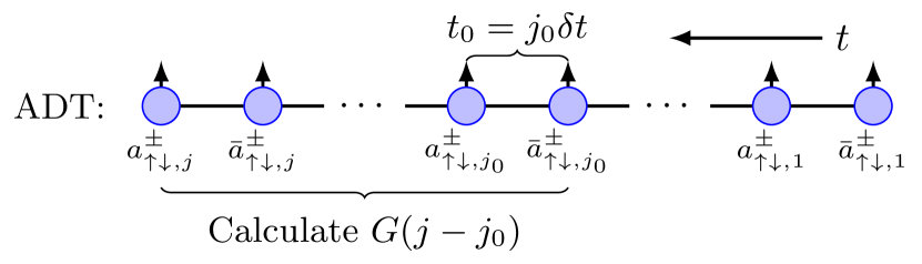
From Eqs. (III.1,34), we can simply use Eqs. (30, 31) to calculate the equilibrium retarded Green’s functions. The only change is to compute those greater and lesser Green’s functions between discrete times $j+j_{0}$ and $k+j_{0}$ instead. This approach is illustrated in Fig. 1. In practice, we find that a relatively small $t_{0}$ is sufficient for the impurity to reach equilibrium (See Sec. IV.2). In addition, to obtain $G_{p,q}(\omega)$ through the Fourier transform of $G_{p,q}(t-t^{\prime})$, one needs to obtain $G_{p,q}(t,t^{\prime})$ for infinitely large $t-t^{\prime}$ in principle. A standard practice is to calculate $G_{p,q}(t,t^{\prime})$ till a finite $t-t^{\prime}$ and then extrapolate the results to infinity, for which we use the well-established linear prediction technique [68, 69]. In this work, we use the same hyperparameter settings for the linear prediction as in Ref. [25].

Our real-time dynamics starts from a separable initial state of the impurity and bath. In principle, for large enough $t_{0}$, the choice of the impurity initial state $\hat{\rho}_{\mathrm{imp}}$ does not matter. However, for numerical calculations, different choices of $\hat{\rho}_{\mathrm{imp}}$ may affect the quality of results due to finite equilibration time $t_{0}$. The effect of $\hat{\rho}_{\mathrm{imp}}$ is fully encoded in the term $\matrixelement{\bm{a}^{+}_{,1}}{\hat{\rho}_{\mathrm{imp}}}{\bm{a}^{-}_{,1}}$ in the expression of $\mathcal{K}$. For simple states, this term can be calculated analytically. For example, for the vacuum state of a spinless fermion with $\hat{\rho}_{\mathrm{imp}}=|0\rangle\langle 0|$, we have

Other than the vacuum state, another natural choice of $\hat{\rho}_{\mathrm{imp}}$ is the impurity thermal state, that is,

For general $\hat{H}_{\rm imp}$, $\matrixelement{\bm{a}^{+}_{,1}}{\hat{\rho}_{\mathrm{imp}}^{{\rm eq}}}{\bm{a}^{-}_{,1}}$ can be calculated using the numerical algorithm shown in Fig. 2. The main idea is to split $\hat{\rho}_{\mathrm{imp}}^{{\rm eq}}$ as $e^{-\beta\hat{H}_{\rm imp}}\approx e^{-\delta\tau\hat{H}_{\rm imp}}\cdots e^{-\delta\tau\hat{H}_{\rm imp}}$ with a small $\delta\tau$, which results in a GMPS after inserting GVs between the imaginary-time propagators (the same as the procedure used to build $\mathcal{K}$ as a GMPS in the imaginary-time GTEMPO method [52]). Then one can easily integrate out all the intermediate GVs to obtain the final expression. This algorithm is very efficient since only the bare impurity dynamics is involved. Therefore one could set $\delta\tau$ to be arbitrarily small to obtain $\matrixelement{\bm{a}^{+}_{,1}}{\hat{\rho}_{\mathrm{imp}}^{{\rm eq}}}{\bm{a}^{-}_{,1}}$ with high precision. For simple impurities such as a single electron, $\matrixelement{\bm{a}^{+}_{,1}}{\hat{\rho}_{\mathrm{imp}}^{{\rm eq}}}{\bm{a}^{-}_{,1}}$ may also be obtained analytically. Nevertheless, the above numeric algorithm is very convenient since it applies for general impurity problems and we found in practice that it is very numerically stable (Analytical expressions can easily run into numerical issues at low temperature if not taken with special care, since a very large $\beta$ appears in the matrix exponential).

Generally, the dominant calculation in the GTEMPO method is the computation of Green’s functions using the zipup algorithm (one can refer to Refs. [51, 52] for details of this algorithm). Concretely, if one represents the IF per flavor as a GMPS (referred to as the MPS-IF) with bond dimension $\chi$, then the computational cost for calculating one Green’s function scales as $O(M\chi_{\mathcal{K}}\chi^{n+1})$ for $n$ flavors [52] ($\chi_{\mathcal{K}}$ is the bond dimension of the GMPS for $\mathcal{K}$ which is usually a small constant). As a result, $\chi$ essentially determines the computational cost of the GTEMPO method.

One major motivation for this work is that the bond dimension $\chi$ involved in the non-equilibrium GTEMPO method is usually much smaller than that in the imaginary-time GTEMPO method. We demonstrate such a difference in bond dimension growth in the non-interacting case with a single flavor. The corresponding non-interacting model is analytically solvable and referred to as the Toulouse model [70] or the Fano-Anderson model [63], with

We will use the square root of the mean square error to quantify the distance between two vectors $\vec{x}$ and $\vec{y}$, denoted as

where $L$ means the length of $\vec{x}$ and $||\cdot||$ means the Euclidean norm. We will refer to $\mathcal{E}(\vec{x},\vec{y})$ as the average error afterwards and neglect the operands of $\mathcal{E}$ when they are clear from the context. In Fig. 3(a,c), we show the imaginary part of the retarded Green’s function calculated by the real-time GTEMPO method, and the Matsubara Green’s function calculated by the imaginary-time GTEMPO method. The corresponding analytical solutions are shown in gray solid lines as comparisons. To clearly show the minimal bond dimensions required in these calculations, we plot the average errors of the real-time and imaginary-time GTEMPO results against the analytical solutions as functions of $\chi$ in Fig. 3(b,d). We can see that the average error saturates around $\chi=40$ in the real-time calculations, but only saturates around $\chi=100$ in the imaginary-time calculations, where the latter is $2.5$ times larger than the former. As a result, for one-orbital impurity models the computational cost of the latter would be $2.5^{3}/4\approx 4$ times higher and for two-orbital impurity models $2.5^{5}/4\approx 25$ times higher, where we have assumed that we evolve till $t=\beta$ in the real-time dynamics and we have already taken into account the fact that the number of GVs in the real-time GTEMPO method is two times larger than the imaginary-time GTEMPO method (generally speaking, the speedup is because that MPS -based algorithms are very sensitive to the bond dimension but only mildly depends on the system size [71]).

For the Toulouse model, it is easy to verify the GTEMPO results against the analytical solutions of the equilibrium Green’s functions. For the single-orbital Anderson impurity model, the analytical solutions do not exist, therefore we verify the GTEMPO results against the state-of-the-art CTQMC results. Since the CTQMC impurity solver is only exact in the imaginary-time axis, we introduce an approach to benchmark the accuracy of our real-time calculations against imaginary-time calculations, that is, we use the spectral function obtained from $G(\omega)$ to calculate $\mathcal{G}(\tau)$, and then compare the obtained $\mathcal{G}(\tau)$ against those calculated using imaginary-time GTEMPO and CTQMC methods.

We present a proof of principle demonstration of the effectiveness of this comparison for the Toulouse model with $\varepsilon_{d}=0$ in Fig. 4(a) and $\varepsilon_{d}=1$ in Fig. 4(b). For the Toulouse model, the retarded Green’s function is independent of the initial state [63], namely $G(t,t^{\prime})=G^{{\rm neq}}(t,t^{\prime})$. Therefore we simply choose $t_{0}=0$ in this case when calculating the equilibrium retarded Green’s function. In both cases, we can see that the $\mathcal{G}(\tau)$ obtained by conversion from $G(t)$ matches very well with the analytical solution.

Now we proceed to consider the single-orbital AIM with

where $\varepsilon_{d}$ is the on-site energy and $U$ is the interaction strength. We will focus on the half-filling case with $\varepsilon_{d}=-U/2$ which gives us an easy first verification of the results, we also set $\beta=40$ ($\Gamma\beta=4$) in all the following calculations.

We first access the quality of the approximate equilibrium state by studying the equilibration dynamics in Fig. 5, where we plot the populations of the impurity in the four states: $|0\rangle$ (no electron), $|\uparrow\rangle$ (spin up), $|\downarrow\rangle$ (spin down) and $|\uparrow\downarrow\rangle$ (double occupancy) as functions of time $t$. We show the results for impurity vacuum state in Fig. 5(a,c,e) and results for impurity thermal state in Fig. 5(b,d,f) respectively, for three different values of $U$ ($U/\Gamma=1,5,10$). We can see that the populations in all these simulations have converged fairly well at $\Gamma t\approx 2$, and that the results for impurity thermal state (which approximately converge around $\Gamma t\approx 1$) clearly converge much faster than those for impurity vacuum state, which indicate that one could use a smaller equilibration time $t_{0}$ if starting from the impurity thermal state (which will significantly reduce the computational cost).

In Fig. 6, we further quantify the error occurred in the retarded Green’s function by using different values of $t_{0}$. Concretely, in Fig. 6(a,c,e), we show $G^{{\rm neq}}(t,t_{0})$ calculated with $\Gamma t_{0}=8$ for $U/\Gamma=1,5,10$ respectively, for both the impurity vacuum state (blue dashed lines) and the impurity thermal state (red dashed lines). We can see that these two lines are completely on top of each other (the average errors are less than $10^{-5}$ for all $U$s). Then in Fig. 6(b,d,f), we take $G^{{\rm neq}}(t,t_{0})$ calculated with $\Gamma t_{0}=8$ as the baseline (which has well reached equilibrium for all the cases we have considered from Fig. 5), and then compute the average error between it and the $G^{{\rm neq}}(t,t_{0})$ calculated with smaller $t_{0}$. We can see that the average errors quickly decrease to less than $10^{-2}$ when $t_{0}$ reaches $\Gamma t_{0}=2$ and saturates at around $\Gamma t_{0}=6$ for both initial states (which is likely due to the first-order time discretization error in Eq.(26)). We can also clearly see that the results for impurity thermal state converge much faster than those for impurity vacuum state.

As application, we plot the spectral function $A(\omega)$ as a function of $\omega$, obtained using different values of $t_{0}$, in Fig. 7(a,c,e) for $U/\Gamma=1,5,10$ respectively, where the red solid lines are results calculated with $\Gamma t_{0}=8$ for impurity thermal state, while the blue and green dashed lines are results calculated with $\Gamma t_{0}=0.5$ for impurity vacuum and thermal states respectively. In Fig. 7(b,d,f), we plot $\mathcal{G}(\tau)$ converted from the $A(\omega)$ calculated in Fig. 7(a,c,e) respectively, where we have also shown the CTQMC results and the imaginary-time GTEMPO results calculated with $\chi=500$ as comparisons. To reduce the finite-time discretization error in this conversion (since we need to perform the Fourier transformation of $G(t)$ in Eq.(13)) we have used a simple linear interpolation scheme to obtain refined real-time data with a smaller time step size $10^{-4}/\Gamma$. We can see that the $\mathcal{G}(\tau)$ converted from $A(\omega)$ calculated with $\Gamma t_{0}=8$ well agrees with the CTQMC and imaginary-time GTEMPO results. Interestingly, the $A(\omega)$ calculated with $\Gamma t_{0}=0.5$ for impurity thermal state agrees fairly well with the $A(\omega)$ calculated with $\Gamma t_{0}=8$ (similar for the corresponding $\mathcal{G}(\tau)$), while in comparison the $A(\omega)$ calculated with $\Gamma t_{0}=0.5$ for impurity vacuum state is very different from that calculated with $\Gamma t_{0}=8$. The insets in Fig. 7(b,d,f) show the average errors between $\mathcal{G}(\tau)$ converted from the $A(\omega)$ calculated with different $t_{0}$ and the imaginary-time GTEMPO results, which decrease at the beginning and saturates at $\Gamma t_{0}\geq 4$ (there is a slight increase of average error for $U/\Gamma=5,10$ when $\Gamma t_{0}$ increases from $1.5$ to $4$, which may be a coincidence due to the errors occurred during the conversion from $A(\omega)$ to $\mathcal{G}(\tau)$). With these results, we can see that the equilibrium retarded Green’s function can indeed be accurately calculated using our method. Moreover, by preparing the initial state of the impurity in a local thermal state, the equilibration time $t_{0}$ can be significantly shortened.