Real-time event simulation with frame-based cameras
Abstract
Event cameras are becoming increasingly popular in robotics and computer vision due to their beneficial properties, e.g., high temporal resolution, high bandwidth, almost no motion blur, and low power consumption. However, these cameras remain expensive and scarce in the market, making them inaccessible to the majority. Using event simulators minimizes the need for real event cameras to develop novel algorithms. However, due to the computational complexity of the simulation, the event streams of existing simulators cannot be generated in real-time but rather have to be pre-calculated from existing video sequences or pre-rendered and then simulated from a virtual 3D scene. Although these offline generated event streams can be used as training data for learning tasks, all response time dependent applications cannot benefit from these simulators yet, as they still require an actual event camera. This work proposes simulation methods that improve the performance of event simulation by two orders of magnitude (making them real-time capable) while remaining competitive in the quality assessment.
SUPPLEMENTARY MATERIAL
The project’s code and additional resources are available at https://cogsys-tuebingen.github.io/realtime_event_simulator/
I INTRODUCTION
In the field of robotics and computer vision, event cameras have been rapidly gaining in popularity. Event cameras work fundamentally differently from traditional frame-based cameras. Instead of capturing an entire frame of pixels at once, an event camera registers log-scale changes in brightness on a pixel level. If the change is large enough, the camera emits an asynchronous event. The advantages of event cameras are that they can register events just microseconds apart, resulting in lower latency and higher temporal resolution ( instead of ) compared to frame-based cameras. These cameras also come with other great potential benefits, such as a high dynamic range and low power consumption [1]. This technology allows for super low latency applications that, when implemented correctly, can leverage all this data to outperform the best traditional computer vision algorithms in various robotics and computer vision tasks. Some useful applications include self-driving cars [2], general purpose object tracking [3], image segmentation [4, 5], high frame rate video reconstruction [6], accurate depth perception [7] and advanced frame interpolation with optical flow reconstruction [8] and robotics applications like control tasks [9], [10], and odometry [11]. For some applications, e.g., self-driving cars [2], it is essential that this data is processed in real-time.
Although the first event camera was released more than a decade ago, event cameras remain expensive (€) and scarce in the market, making them inaccessible to many researchers, companies, and hobbyists alike. This work proposes using frame-based cameras to simulate this event data. Traditional frame-based cameras remain cheap and readily available, making this approach an interesting alternative.
Over the last few years, several methods have been published that attempt to simulate event data. While these recent publications produce great results of high quality in the event simulation, the computation required for just one frame can take up to multiple seconds, eliminating the possibility of real-time use. To truly use a frame-based camera as a replacement for an event camera in robotics applications, these simulators would have to run at much higher speeds.
This work specifically attempts to address this problem by presenting methods that aim to drastically improve the runtime of these simulations while remaining competitive in quality, to be of use for real-time robotics applications.
Contributions of this work are as follows:
-
•
Optical flow based event simulation methods running in real-time
-
•
A novel event simulation method which leverages the sparsity of events in the interpolation to further improve the runtime
-
•
Qualitative and quantitative results comparing our event simulation methods with existing ones and real event cameras, and a guideline, when to use which simulator
The rest of the paper is organized as follows: Section II presents the related work. In Section III we present our methods. In Section IV we present qualitative and quantitative comparisons. Conclusions are drawn in Section V.
II RELATED WORK
One of the first event simulators was described in [12]. This event simulator subtracts consecutive frames and afterward applies a threshold to retain only pixels that have a significant difference. The approach in [13] is also based on subtracting frames, however, their contribution is the differentiability of the event simulator, which is needed for backpropagation. While our approach subtracts consecutive frames, we use optical flow to interpolate the given input frames, leading to a temporal resolution closer to one of the real event cameras. Approaches such as [14], [15], and [16] use a rendering engine to capture images from a 3D scene.
In [17], the authors developed an event simulator tightly coupled with the rendering engine to adaptively sample the visual signal from the virtual camera sensor along a given camera trajectory. This allows generating simulated events asynchronously, whereas previous simulators only provide synchronous events. This approach also simulates some linear noise but neglects non-linear noise. In [18], the authors extended their previous work [17] by combining it with a frame interpolation method to generate events from videos. Similar to [18], [19] converts regular video sequences to events. Compared to previous work, [19] includes more realistic noise models and therefore comes closer to the output of real event cameras. In [20], the authors go one step further and add several improvements and additions. The model notably improves the noise simulation by directly mapping noise distributions from real pixels. In another recent approach, the authors developed a GAN-style neural network to regress an event volume (an event representation) [21]. To train the network, two consecutive frames and the corresponding events were given. On inference time, only two consecutive frames are needed. While the approach can approximate the true noise distributions of real events more accurately, it does not seem to run in real-time, and the output is an event representation and not the events themselves.
Most of the existing event simulators focus on the realistic event output of the simulator. This comes at the cost of a high computational load, and therefore an increased runtime. For many applications, especially learning-based solutions, such event simulators are ideal. However, many robotics applications favor real-time capability over realistic events with accurate noise. Our event simulators have a less realistic noise model, but do run in real-time while remaining competitive in quality. To the best of our knowledge, this work presents the first method to simulate events given the output of a frame-based camera in real-time.
III METHOD
We present three different methods to simulate events. All of them are based on the subtraction of consecutive frames, as done in [12]. We call the result of the subtraction the difference frame. In contrast to event cameras, we do not use the log difference but the linear difference. The quality improvement of log differences is small and comes with a high computational load (delay in ms depending on the interpolated frames). Further, this work does not address the noise and artifacts present in data from a real event camera.
The temporal resolution of frame-based cameras is much lower than that of event cameras [1]. To counteract this, we use interpolation to artificially increase the frame rate. Interpolation is a common step in event simulation and is also used in [18] and [19]. For interpolation, we use optical flow algorithms and a simple but fast linear interpolation approach. We used the fastest optical flow algorithms evaluated in [22].
Next follows the detailed description of the three methods. In Section III-A, we describe a method based on dense frame interpolation. Section III-B introduces a method that uses sparse frame interpolation, and the technique described in Section III-C interpolates only the difference frames.
III-A DENSE FRAME INTERPOLATION
This method calculates the dense optical flow between two consecutive camera frames in the first step. This dense optical flow is then used to interpolate between the two consecutive camera frames. Given these interpolated frames, consecutive frames are subtracted to get difference frames. In the last step, the difference frames are thresholded (with and ) to determine all the pixels that should emit an event, and the corresponding polarity of the event according to
The process of this approach is illustrated in Fig. 1.
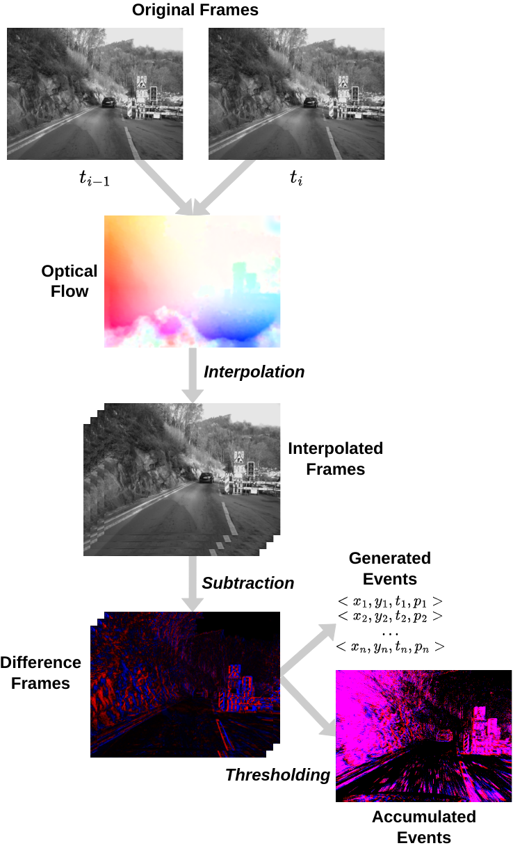
The output is either the events in tuples of the form with the location of the event , the time stamp and the polarity of the event or a frame with the accumulated events.
In order to use this algorithm in real-time applications, the choice of the dense optical flow algorithm is very important, as its speed is the main bottleneck for the performance of this method.
III-B SPARSE FRAME INTERPOLATION
This method is similar to the dense frame interpolation approach described in Section III-A with the difference that sparse optical flow is used to interpolate between two consecutive camera frames.
The motivation to use sparse optical flow is to increase the performance by reducing the number of calculations for the frame interpolation step. Dense optical flow algorithms consider the entire frame while only a fraction of the pixels in a frame is actually changing a lot, most of the time. Real event cameras use a threshold to detect when an event at a particular pixel has occurred. Analogously to an event camera, all pixels that have not changed within a given threshold from one frame to the next can be disregarded for the optical flow estimation. This way, the computation can be sped up as long as the number of pixels that have changed is substantially lower than the total number of pixels in the frame. The selected pixels can be estimated with any sparse optical flow algorithm.
It is important to note that sparse optical flow estimations are usually slower than dense algorithms per pixel, so this algorithm benefits from static backgrounds containing small moving subjects.
III-C DIFFERENCE FRAME INTERPOLATION
Interpolating regular frames is a complex problem with many unforeseen edge cases such as, e.g., occlusions, and is computationally expensive. Traditional interpolation algorithms all rely on the basic assumption that the area of pixels that make up an object will not change drastically in color, brightness, or size from one frame to another. This assumption breaks down in scenes where occlusions occur. Traditional optical flow algorithms cannot find the original pixels, and artifacts appear in the optical flow estimation.
To reduce the possibility of such edge cases and to further decrease the computational load of the interpolation step, this approach only interpolates between consecutive difference frames rather than between consecutive camera frames. This method reduces complexity by only interpolating between the events themselves since we assume that the difference frames represent the events.
Given three consecutive camera frames, two difference frames are calculated in the first step. The optical flow between the two difference frames is calculated in the next step. With this optical flow, additional difference frames can be interpolated between the two difference frames, from the first step. The process of this approach is illustrated in Fig. 2.

This method makes some strict assumptions about the original frame sequence. The objects’ movement that generates events must be of constant linear velocity. Furthermore, the perspective of these objects in the video cannot change over time. Given these assumptions, this method is specially targeted for tasks like, e.g., object tracking.
IV EVALUATION
We evaluate our proposed simulation methods in three different ways. We start in Section IV-A with a comparison of the runtimes of the different event simulation methods. In Section IV-B, we qualitatively compare the output of our methods to real events and the output of another event simulator. Next to the qualitative comparison, we compare some statistics of the simulated, the real events, and two other event simulators in Section IV-C.
IV-A RUNTIMES
We compare the runtimes of our proposed event simulation methods in two different scenarios. The first scenario is a dynamic scene with a high events-per-frame ratio. This footage is taken from [23]. The dataset contains recorded events and camera frames at fps from a car driving around. We took a frame sequence with frames from the interlaken_00_c sequence. The frames with an original resolution of pixels were resized to the resolution of the event camera ( pixels) before passing it to the event simulators. For this dataset, we used interpolated (difference) frames. The results of this experiment are shown in Fig. 3.
We use a less dynamic scene with a low events-per-frame ratio in the second scenario. Specifically, we recorded a flying table tennis ball in front of a static background with a FLIR CHAMELEON 3 camera at fps and a Prophesee Gen4 event camera [24]. This frame sequence contains frames. We also resized the input frames for this dataset from pixels (the camera’s resolution) to pixels (the resolution of the event camera), before passing it to the event simulators. For this dataset, we used interpolated (difference) frames. The results of this experiment are shown in Fig. 4.
Next to the runtimes of our three proposed methods, we also list the runtimes for calculating the difference frame as a reference. We also compare our event simulation methods to vid2e [18] and v2e [19], two state-of-the-art event simulators.
We used different optical flow algorithms for all three event simulation methods since the simulation methods heavily depend on the used optical flow implementation.
We chose , , and the number of interpolated frames so that the generated events resemble the ground truth accumulated event frame. These values are listed in Table I.
| Method | # int. frames | ||
|---|---|---|---|
| Dense interpolation | 2 | -2 | 10 |
| Sparse interpolation | 10 | -10 | 10 |
| Difference interpolation | 20 | -20 | 10 |
| v2e [19] | 0.3 | -0.3 | ? |
| vid2e [18] | 0.2 | -0.2 | ? |
All the experiments were run on a desktop with an Intel i7 9700 3.0 GHz CPU, 32GB RAM, and an NVIDIA GeForce RTX 2080 Ti. For each algorithm, the video sequence was loaded into RAM before the time was measured. Then the entire video is passed to each algorithm frame by frame. After the last frame, the time measurement was stopped. We recorded the runtimes of 10 runs. From these, the mean runtime and the standard deviation were calculated.


Discussion As can be seen in the results shown in Fig. 3 and Fig. 4, the runtimes differ substantially depending on the event simulation method and their configuration.
Starting with the dynamic dataset, the dense interpolation method with DIS [22] on its lowest quality setting is the fastest configuration for the dense approach, closely followed by the one with Farneback [25] (on the GPU). DIS takes more than three times as long with the highest quality setting. The sparse interpolation method on the GPU is a bit slower than the dense one. The sparse interpolation method on the CPU performs the worst of all the techniques with different settings. Since there is a lot of movement in this driving car dataset, we expect the sparse interpolation method to be worse. As mentioned in Section III-B, sparse optical flow benefits only if the number of pixels that have changed is substantially lower than the total number of pixels. In this experiment, this is not the case. The GPU and CPU runtimes of the difference interpolation method are better compared to the corresponding runtimes of the sparse interpolation method, with the GPU version outperforming the CPU version.
On the less dynamic dataset, the runtimes for the dense interpolation method are all longer because the resolution of the table tennis video is larger ( pixels compared to pixels). For the dense interpolation method, the relative comparisons remain the same. As can be seen in Fig. 4, with runtimes above 80ms, the dense optical flow algorithms are too slow to be used in real-time applications in such scenarios. However, the dense method with DIS with the high quality preset is still three orders of magnitude faster than vid2e [18] and v2e [19]. Since there is only one moving ball in front of a static background in this dataset, the sparse interpolation method only needs to estimate the motion of the pixels representing the ball. As expected, the sparse interpolation method performs very well. The difference interpolation method, with its strict assumption met on this dataset, achieves the best runtimes.
IV-B QUALITATIVE COMPARISON
For qualitative comparison, the outputs of the different methods are shown in Fig. 5 for the dynamic dataset and in Fig. 6 for the less dynamic dataset. We used the same datasets as in Section IV-A. The accumulation time was set to mimic the frame rate of the frame camera ().
Discussion Starting with the dynamic dataset, the output of the dense interpolation methods, shown in Figs. 5f, 5i, 5d and 5e, bear a very strong resemblance to the ground truth accumulated event frame, shown in Fig. 5b. The positive and negative overlapping events, missing in the difference frame (Fig. 5c), are primarily generated from the interpolation. The impact of the different optical flow algorithms is relatively small, with the main difference being the amount of motion registered in the street area of the frames. The output of the sparse interpolation methods, shown in Figs. 5g and 5j, also bear a very strong resemblance to the ground truth accumulated event frame, shown in Fig. 5b. The output is noticeably noisier than the one of the dense interpolation methods, which is to be expected because of the sparse interpolation. If neighboring pixels are just under the threshold, they will not be interpolated and therefore do not emit an event. Additionally, some artifacts appear when Lucas Kanade [26] is run on the GPU. These artifacts are probably a side product because only patches of the original image are sent to the GPU by OpenCV. The difference interpolation method performs quite poorly on this dataset, as can be seen in Figs. 5h and 5k. This is mainly due to the constraints not being met. The perspective of the objects in the scene changes quite drastically as the car is driving by them. However, some events between the two frames are still emitted, and the output is a clear improvement over the simple difference frame. The output of v2e comes closest to the one of the difference interpolation method from a visual point of view.
In the less dynamic dataset, the dense interpolation method does not perform as well, shown in Figs. 6f, 6i, 6d and 6e. The dense interpolation method with DIS with the low-quality preset cannot even detect any motion, making the ball completely invisible, as seen in Fig. 6d. With the Farneback optical flow algorithm, the dense interpolation method manages to estimate some motion in the ball but creates an event cloud around it (Figs. 6f and 6i). Only the dense interpolation method with DIS on the high-quality preset produces a favorable result, as seen in Fig. 6e. These inaccuracies can be attributed to the dense optical flow algorithms. Traditional dense optical flow algorithms find the frame’s general motion in patches. This is especially a problem for DIS [22] with the low quality preset as the ball is not even registered because of the large patch size and the fact that the surrounding pixels do not move with the ball. The output of the sparse interpolation method has some artifacts due to the interpolation of overlapping subjects. One object represents where the ball has moved in the current frame, and one object where the ball was in the previous frame. The GPU implementation has some additional artifacts similar to the ones in the dynamic dataset. The output of the difference interpolation, shown in Figs. 6h and 6k, makes it apparent that this method is well suited for this kind of scene. It is the only algorithm able to correctly interpolate the ball’s position and create the events that lie between the two frames. As seen in Fig. 6l, v2e produces quite some artifacts and does not look as similar to the ground truth compared to most of our methods.
IV-C STATISTICAL COMPARISON
In this section, we present a statistical comparison of our event simulation methods with real events and the output of vid2e [18] and v2e [19]. We use the metric of events per pixel per second introduced in [27] as comparison for two short sequences. Event count is a necessary but not sufficient condition for a faithful simulation of an event camera. We took ( frames) from the interlaken_00_c sequence from [23] for high events-per-frame data and ( frames) from our flying table tennis ball dataset for low events-per-frame data. We adjusted the threshold values and for every simulation method to get similar mean values as the ones from the real events. We list the mean and standard deviation as well as the used threshold values and (unless unknown) in Table II for the high events-per-frame data and in Table III for the low events-per-frame data.
Discussion As can be seen in Table II, for the high events-per-frame dataset, our simulation methods tend to have a bit of a lower standard deviation compared to the real events, v2e and vid2e. On the low events-per-frame dataset, however, most of our simulation methods have standard deviations closer to the one of the real events compared to v2e and vid2e.
| Events / (pixel s) | ||||
|---|---|---|---|---|
| Method | mean | std. dev. | ||
| Real events | 62.7933 | 82.7128 | ? | ? |
| Dense int. w. DIS, lq. preset | 56.3079 | 58.9868 | 3 | -3 |
| Dense int. w. DIS, hq. preset | 65.6304 | 66.793 | 3 | -3 |
| Dense int. w. Farneback | 65.999 | 67.4279 | 3 | -3 |
| Sparse int. w. LK | 59.3083 | 52.3827 | 6 | -6 |
| Difference int. w. LK | 59.3034 | 55.0075 | 19 | -19 |
| v2e [19] | 58.8313 | 78.3513 | 0.1 | 0.1 |
| vid2e [18] | 63.6588 | 77.9866 | 0.14 | 0.14 |
| Events / (pixel s) | ||||
|---|---|---|---|---|
| Method | mean | std. dev. | ||
| Real events | 0.046 | 1.0228 | 43 | -17 |
| Dense int. w. DIS, lq. preset | 0.0472 | 1.165 | 13 | -13 |
| Dense int. w. DIS, hq. preset | 0.0462 | 0.8783 | 35 | -35 |
| Dense int. w. Farneback | 0.0445 | 0.574 | 19 | -19 |
| Sparse int. w. LK | 0.0467 | 0.439 | 27 | -27 |
| Difference int. w. LK | 0.0461 | 0.8785 | 112 | -112 |
| v2e [19] | 0.0455 | 0.4912 | 0.575 | 0.575 |
| vid2e [18] | 0.0318 | 1.776 | 5.7 | -5.7 |
V CONCLUSION
This work presented multiple event simulator methods that can run in under ms. Compared to existing event simulators, ours can be used in real-time robotics applications while remaining competitive in the quality assessment. We have shown the influence of the resolution and the dynamics of the scene on the runtime of the simulators, the quality of the simulated events, and the statistics of the events.
Depending on the camera setup and the dynamics of the scene, we have the following suggestions: For scenes with high dynamics, e.g., an event camera mounted on a driving car, we recommend the dense interpolation method with Farneback on the GPU. In scenes with fewer dynamics, e.g., tracking an object with a static event camera, we recommend using the difference interpolation method. For use cases in between, some experiments might be needed to find the sweet spot between a fast runtime and a high quality of the simulated events. The sparse interpolation method might be a good choice.
With this work, we have made a first step towards event simulators for real-time robotics applications. We hope our work enables others to develop new algorithms for event-based data in real-time use cases.
References
- [1] G. Gallego, T. Delbrück, G. Orchard, C. Bartolozzi, B. Taba, A. Censi, S. Leutenegger, A. J. Davison, J. Conradt, K. Daniilidis, and D. Scaramuzza, “Event-based vision: A survey,” IEEE Transactions on Pattern Analysis and Machine Intelligence, vol. 44, no. 1, pp. 154–180, 2022.
- [2] A. I. Maqueda, A. Loquercio, G. Gallego, N. García, and D. Scaramuzza, “Event-based vision meets deep learning on steering prediction for self-driving cars,” in 2018 IEEE/CVF Conference on Computer Vision and Pattern Recognition, 2018, pp. 5419–5427.
- [3] E. Perot, P. de Tournemire, D. Nitti, J. Masci, and A. Sironi, “Learning to detect objects with a 1 megapixel event camera,” in Advances in Neural Information Processing Systems, H. Larochelle, M. Ranzato, R. Hadsell, M. F. Balcan, and H. Lin, Eds., vol. 33. Curran Associates, Inc., 2020, pp. 16 639–16 652. [Online]. Available: https://proceedings.neurips.cc/paper/2020/file/c213877427b46fa96cff6c39e837ccee-Paper.pdf
- [4] I. Alonso and A. C. Murillo, “Ev-segnet: Semantic segmentation for event-based cameras,” in IEEE International Conference on Computer Vision and Pattern Recognition Workshops (CVPRW), 2019.
- [5] Y. Zhou, G. Gallego, X. Lu, S. Liu, and S. Shen, “Event-based motion segmentation with spatio-temporal graph cuts,” IEEE Transactions on Neural Networks and Learning Systems, pp. 1–13, 2021.
- [6] L. Pan, R. Hartley, C. Scheerlinck, M. Liu, X. Yu, and Y. Dai, “High frame rate video reconstruction based on an event camera,” IEEE Transactions on Pattern Analysis and Machine Intelligence, pp. 1–1, 2020.
- [7] M. Muglikar, D. P. Moeys, and D. Scaramuzza, “Event guided depth sensing,” in 2021 International Conference on 3D Vision (3DV), 2021, pp. 385–393.
- [8] S. Tulyakov, D. Gehrig, S. Georgoulis, J. Erbach, M. Gehrig, Y. Li, and D. Scaramuzza, “Time lens: Event-based video frame interpolation,” in Proceedings of the IEEE/CVF Conference on Computer Vision and Pattern Recognition (CVPR), June 2021, pp. 16 155–16 164.
- [9] R. S. Dimitrova, M. Gehrig, D. Brescianini, and D. Scaramuzza, “Towards low-latency high-bandwidth control of quadrotors using event cameras,” in IEEE International Conference on Robotics and Automation (ICRA). IEEE, May 2020. [Online]. Available: https://doi.org/10.1109/icra40945.2020.9197530
- [10] A. Vitale, A. Renner, C. Nauer, D. Scaramuzza, and Y. Sandamirskaya, “Event-driven vision and control for UAVs on a neuromorphic chip,” in 2021 IEEE International Conference on Robotics and Automation (ICRA). IEEE, May 2021. [Online]. Available: https://doi.org/10.1109/icra48506.2021.9560881
- [11] J. Hidalgo-Carrió, G. Gallego, and D. Scaramuzza, “Event-aided direct sparse odometry,” in IEEE Conference on Computer Vision and Pattern Recognition (CVPR), 2022.
- [12] J. Kaiser, J. C. V. Tieck, C. Hubschneider, P. Wolf, M. Weber, M. Hoff, A. Friedrich, K. Wojtasik, A. Roennau, R. Kohlhaas, R. Dillmann, and J. M. Zollner, “Towards a framework for end-to-end control of a simulated vehicle with spiking neural networks,” in 2016 IEEE International Conference on Simulation, Modeling, and Programming for Autonomous Robots (SIMPAR). IEEE, Dec. 2016. [Online]. Available: https://doi.org/10.1109/simpar.2016.7862386
- [13] J. Nehvi, V. Golyanik, F. Mueller, H.-P. Seidel, M. Elgharib, and C. Theobalt, “Differentiable event stream simulator for non-rigid 3d tracking,” in CVPR Workshop on Event-based Vision, 2021.
- [14] E. Mueggler, H. Rebecq, G. Gallego, T. Delbruck, and D. Scaramuzza, “The event-camera dataset and simulator: Event-based data for pose estimation, visual odometry, and SLAM,” The International Journal of Robotics Research, vol. 36, no. 2, pp. 142–149, Feb. 2017. [Online]. Available: https://doi.org/10.1177/0278364917691115
- [15] W. Li, S. Saeedi, J. McCormac, R. Clark, D. Tzoumanikas, Q. Ye, Y. Huang, R. Tang, and S. Leutenegger, “Interiornet: Mega-scale multi-sensor photo-realistic indoor scenes dataset,” in British Machine Vision Conference (BMVC), 2018.
- [16] A. Radomski, A. Georgiou, T. Debrunner, C. Li, L. Longinotti, M. Seo, M. Kwak, C.-W. Shin, P. K. J. Park, H. E. Ryu, and K. Eng, “Enhanced frame and event-based simulator and event-based video interpolation network,” 2021. [Online]. Available: https://arxiv.org/abs/2112.09379
- [17] H. Rebecq, D. Gehrig, and D. Scaramuzza, “ESIM: an open event camera simulator,” Conf. on Robotics Learning (CoRL), Oct. 2018.
- [18] D. Gehrig, M. Gehrig, J. Hidalgo-Carrio, and D. Scaramuzza, “Video to events: Recycling video datasets for event cameras,” in 2020 IEEE/CVF Conference on Computer Vision and Pattern Recognition (CVPR). IEEE, Jun. 2020. [Online]. Available: https://doi.org/10.1109/cvpr42600.2020.00364
- [19] Y. Hu, S. C. Liu, and T. Delbruck, “v2e: From video frames to realistic DVS events,” in 2021 IEEE/CVF Conference on Computer Vision and Pattern Recognition Workshops (CVPRW). IEEE, 2021. [Online]. Available: http://arxiv.org/abs/2006.07722
- [20] D. Joubert, A. Marcireau, N. Ralph, A. Jolley, A. van Schaik, and G. Cohen, “Event camera simulator improvements via characterized parameters,” Frontiers in Neuroscience, vol. 15, Jul. 2021. [Online]. Available: https://doi.org/10.3389/fnins.2021.702765
- [21] A. Z. Zhu, Z. Wang, K. Khant, and K. Daniilidis, “Eventgan: Leveraging large scale image datasets for event cameras,” 2019. [Online]. Available: https://arxiv.org/abs/1912.01584
- [22] T. Kroeger, R. Timofte, D. Dai, and L. V. Gool, “Fast optical flow using dense inverse search,” in Computer Vision – ECCV 2016. Springer International Publishing, 2016, pp. 471–488. [Online]. Available: https://doi.org/10.1007/978-3-319-46493-0_29
- [23] M. Gehrig, W. Aarents, D. Gehrig, and D. Scaramuzza, “DSEC: A stereo event camera dataset for driving scenarios,” IEEE Robotics and Automation Letters, vol. 6, no. 3, pp. 4947–4954, Jul. 2021. [Online]. Available: https://doi.org/10.1109/lra.2021.3068942
- [24] T. Finateu, A. Niwa, D. Matolin, K. Tsuchimoto, A. Mascheroni, E. Reynaud, P. Mostafalu, F. Brady, L. Chotard, F. LeGoff, H. Takahashi, H. Wakabayashi, Y. Oike, and C. Posch, “5.10 a 1280×720 back-illuminated stacked temporal contrast event-based vision sensor with 4.86m pixels, 1.066geps readout, programmable event-rate controller and compressive data-formatting pipeline,” in 2020 IEEE International Solid- State Circuits Conference - (ISSCC). IEEE, Feb. 2020. [Online]. Available: https://doi.org/10.1109/isscc19947.2020.9063149
- [25] G. Farnebäck, “Two-frame motion estimation based on polynomial expansion,” in Image Analysis. Springer Berlin Heidelberg, 2003, pp. 363–370. [Online]. Available: https://doi.org/10.1007/3-540-45103-x_50
- [26] B. D. Lucas and T. Kanade, “An iterative image registration technique with an application to stereo vision,” in Proceedings of the 7th International Joint Conference on Artificial Intelligence - Volume 2, ser. IJCAI’81. San Francisco, CA, USA: Morgan Kaufmann Publishers Inc., 1981, p. 674–679.
- [27] T. Stoffregen, C. Scheerlinck, D. Scaramuzza, T. Drummond, N. Barnes, L. Kleeman, and R. Mahoney, “Reducing the sim-to-real gap for event cameras,” in European Conference on Computer Vision (ECCV), august 2020.