Reactive Message Passing for Scalable Bayesian Inference
Abstract
We introduce Reactive Message Passing (RMP) as a framework for executing schedule-free, robust and scalable message passing-based inference in a factor graph representation of a probabilistic model. RMP is based on the reactive programming style that only describes how nodes in a factor graph react to changes in connected nodes. The absence of a fixed message passing schedule improves robustness, scalability and execution time of the inference procedure. We also present ReactiveMP.jl, which is a Julia package for realizing RMP through minimization of a constrained Bethe free energy. By user-defined specification of local form and factorization constraints on the variational posterior distribution, ReactiveMP.jl executes hybrid message passing algorithms including belief propagation, variational message passing, expectation propagation, and expectation maximisation update rules. Experimental results demonstrate the improved performance of ReactiveMP-based RMP in comparison to other Julia packages for Bayesian inference across a range of probabilistic models. In particular, we show that the RMP framework is able to run Bayesian inference for large-scale probabilistic state space models with hundreds of thousands of random variables on a standard laptop computer.
Keywords
Bayesian Inference, Factor Graphs, Message Passing, Reactive Programming, Variational Inference
1 Introduction
In this paper, we develop a reactive approach to Bayesian inference on factor graphs. We provide the methods, implementation aspects, and simulation results of message passing-based inference realized by a reactive programming paradigm. Bayesian inference methods facilitate the realization of a very wide range of useful applications, but in our case, we are motivated by our interest in execution real-time Bayesian inference in state space models with data streams that potentially may deliver an infinite number of observations over an indefinite period of time.
The main idea of this paper is to combine message passing-based Bayesian inference on factor graphs with a reactive programming approach to build a foundation for an efficient, scalable, adaptable, and robust Bayesian inference implementation. Efficiency implies less execution time and less memory consumption than alternative approaches; scalability refers to running inference in large probabilistic models with possibly hundreds of thousands of random variables; adaptability implies real-time in-place probabilistic model adjustment, and robustness relates to protection against failing sensors and missing data. We believe that the proposed approach, which we call Reactive Message Passing (RMP), will lubricate the transfer of research ideas about Bayesian inference-based agents to real-world applications. To that end, we have developed and also present ReactiveMP.jl, which is an open source Julia package that implements RMP on a factor graph representation of a probabilistic model. Our goal is that ReactiveMP.jl grows to support practical, industrial applications of inference in sophisticated Bayesian agents and hopefully will also drive more research in this area.
In Section 2, we motivate the need for RMP by analysing some weaknesses of alternative approaches. Section 3 reviews background knowledge on message passing-based inference on factor graphs and variational Bayesian inference as a constrained Bethe free energy optimisation problem. The rest of the paper discusses our main contributions:
-
•
In Section 4, we present the idea of Reactive Message Passing as a way to perform event-driven reactive Bayesian inference by message passing in factor graphs. RMP is a surprisingly simple idea of combining two well-studied approaches from different fields: message passing-based Bayesian inference and reactive programming;
-
•
In Section 5, we present an efficient and scalable implementation of RMP for automated Bayesian inference in the form of the ReactiveMP.jl package for the Julia programming language. We also introduce a specification language for the probabilistic model and inference constraints;
-
•
In Section 6, we benchmark the ReactiveMP.jl on various standard probabilistic signal processing models and compare it with existing message passing-based and sampling-based Bayesian inference implementations. We show that our new implementation scales easily for conjugate state space models that include hundreds of thousands random variables on a regular MacBook Pro laptop computer. For these models, in terms of execution time, memory consumption, and scalability, the proposed RMP implementation Bayesian inference outperforms the existing solutions by hundreds orders of magnitude and takes roughly a couple of milliseconds or a couple of minutes depending on the size of a dataset and a number of random variables in a model.
Finally, in Section 7 we discuss work-in-progress and potential future research directions.
2 Motivation
Open access to efficient software implementations of strong mathematical or algorithmic ideas often leads to sharply increasing advances in various practical fields. For example, backpropagation in artificial neural networks stems from at least the 1980’s, but practical applications have skyrocketed in recent years due to new solutions in hardware and corresponding software implementations such as TensorFlow (Martín Abadi et al., 2015) or PyTorch (Paszke et al., 2019).
However, the application of Bayesian inference for real-world signal processing problems still remains a big challenge. If we consider an autonomous robot that tries to find its way in a new terrain, we would want it to reason about its environment in real-time as well as to be robust to potential failures in its sensors. Furthermore, the robot preferably has the ability to not only to adapt to new observations, but also to adjust its internal representation of the current environment in real-time. Additionally, the robot will have limited computational capabilities and should be energy-efficient. These issues form a very challenging barrier in the deployment of real-time Bayesian inference-based synthetic agents to real-world problems.
In this paper, our goal is to build a foundation for a new approach to efficient, scalable, and robust Bayesian inference in state space models and release an open source toolbox to support the development process. By efficiency, we imply the capability of performing real-time Bayesian inference with a limited computational and energy budget. By scalability, we mean inference execution to acceptable accuracy with limited resources, even if the model size and number of latent variables gets very large. Robustness is also an important feature, by which we mean that if the inference system is deployed in a real-world setting, then it needs to stay continually operational even if part of the system collapses.
We propose a combination of message passing-based Bayesian inference on Forney-style Factor Graphs and the reactive programming approach, which, to our knowledge, is less well-known and new in the message passing literature. Our approach is inspired by the neuroscience community and the Free Energy Principle (Friston, 2009) since the brain is a good example of a working system that already realizes real-time and robust Bayesian inference at a large scale for a small energy consumption budget.
Message passing
Generative models for complex real-world signals such as speech or video streams are often described by highly factorised probabilistic models with sparse structure and few dependencies between latent variables. Bayesian inference in such models can be performed efficiently by message passing on the edges of factor graphs. A factor graph visualizes a factorised representation of a probabilistic model where edges represent latent variables and nodes represent functional dependencies between these variables. Generally, as the models scale up to include more latent variables, the fraction of direct dependencies between latent variables decreases and as a result the factor graph becomes sparser. For highly factorized models, efficient inference can be realized by message passing as it naturally takes advantage of the conditional independencies between variables.
Existing software packages for message passing-based Bayesian inference, such as ForneyLab.jl (van de Laar et al., 2018) and Infer.Net (Minka et al., 2018), have been implemented in an imperative programming style. Before the message passing algorithm in these software packages can be executed, a message passing schedule (i.e., the sequential order of messages) needs to be specified (Elidan et al., 2012; Bishop, 2006). In our opinion, an imperative coding style and reliance on a pre-specified message schedule might be problematic from a number of viewpoints. For example, a fixed pre-computed schedule requires a full analysis of the factor graph that corresponds to the model, and if the model structure adapts, for instance, by deleting a node, then we are forced to stop the system and create a new schedule. This restriction makes it hard to deploy these systems in the field, since either we abandon model structure optimization or we give up on the guarantee that the system is continually operational. In addition, in real-world signal processing applications, the data often arrives asynchronously and may have significantly different update rates in different sensory channels. A typical microphone has a sample rate of 44.1 kHz, whereas a typical video camera sensor has a sample rate of 30-60 Hz. These factors create complications since an explicitly sequential schedule-based approach requires an engineer to create different schedules for different data sources and synchronise them explicitly, which may be cumbersome and error-prone.
Reactive programming
In this paper, we provide a fresh look on message passing-based inference from an implementation point of view. We explore the feasibility of using the reactive programming (RP) paradigm as a solution for the problems stated above. Essentially, RP supports to run computations by dynamically reacting to changes in data sources, thus eliminating the need for a pre-computed synchronous message update scheme. Benefits of using RP for different problems have been studied in various fields starting from physics simulations (Boussinot et al., 2015) to neural networks (Busch et al., 2020) and probabilistic programming as well (Baudart et al., 2019). We propose a new reactive version of message passing framework, which we simply call Reactive Message Passing (RMP). The new message passing-based inference framework is designed to run without any pre-specified schedule, autonomously reacts to changes in data, scales to large probabilistic models with hundreds of thousands of unknowns, and, in principle, allows for more advanced features, such as run-time probabilistic model adjustments, parallel inference execution, and built-in support for asynchronous data streams with different update rates.
To support further development we present our own implementation of the RMP framework in the form of a software package for the Julia programming language called ReactiveMP.jl. We show examples and benchmarks of the new implementation for different probabilistic models including a Gaussian linear dynamical system, a hidden Markov model and a non-conjugate hierarchical Gaussian filter model. More examples including mixture models, autoregressive models, Gaussian flow models, real-time processing, update rules based on the expectation propagation algorithm, and others are available in the ReactiveMP.jl repository on GitHub.
3 Background
This section first briefly introduces message passing-based exact Bayesian inference on Forney-style Factor Graphs. Then, we extend the scope to approximate Bayesian inference by Variational Message Passing based on minimisation of the Constrained Bethe Free Energy.
Forney-style Factor Graphs
In our work, we use Terminated Forney-style Factor Graphs (TFFG) (Forney, 2001) to represent and visualise conditional dependencies in probabilistic models, but the concept of RMP should be compatible with all other graph-based model representations. For good introductions to Forney-style factor graphs, we refer the reader to Loeliger (2004); Korl (2005).
Inference by Message Passing
We consider a probabilistic model with probability density function where represents observations and represents latent variables. The general goal of Bayesian inference is to estimate the posterior probability distribution . Often, it is also useful to estimate marginal posterior distributions
| (1) |
for the individual components of . In the case of discrete states or parameters, the integration is replaced by a summation.
In high-dimensional spaces, the computation of (1) quickly becomes intractable, due to an exponential explosion of the size of the latent space (Bishop, 2006). The TFFG framework provides a convenient solution for this problem. As a simple example, consider the factorised distribution
| (2) |
This model can be represented by a TFFG shown in Fig. 1. The underlying factorisation of allows the application of the algebraic distributive law, which simplifies the computation of (1) to a nested set of lower-dimensional integrals as shown in (3), which effectively reduces the exponential complexity of the computation to linear. In the corresponding TFFG, these nested integrals can be interpreted as messages that flow on the edges between nodes.
| (3) |

The resulting marginal in (3) is simply equal to the product of two incoming (or colliding) messages on the same edge, divided by the normalisation constant
| (4) |
This procedure for computing a posterior distribution is known as the Belief Propagation (BP) or Sum-Product (SP) message passing algorithm and it requires only the evaluation of low-dimensional integrals over local variables. In some situations, for example when all incoming messages are Gaussian and the node function is linear, it is possible to use a closed-form analytical solutions for the messages. These closed-form formulas are also known as message update rules.
Variational Bayesian inference
Inference problems in practical models often involve computing messages in (4) which are difficult to evaluate analytically. In these cases, we may resort to approximate Bayesian inference solutions with the help of variational Bayesian inference methods (Winn, 2003; Dauwels, 2007). In general, the variational inference procedure introduces a variational posterior that acts as an approximating distribution to the Bayesian posterior . The set is called a variational family of distributions. Typically, in variational Bayesian inference methods the aim is minimize the Variational Free Energy (VFE) functional
| (5) | ||||
| (6) |
In most cases, additional constrains on the set make the optimisation task (6) computationally more efficient than the belief propagation but only gives an approximate solution for (1). The literature distinguishes two major types of constraints on : form constraints and factorisation constraints (Şenöz et al., 2021). Form constraints force the approximate posterior or its marginals to be of a specific parametric functional form, e.g., a Gaussian distribution . Factorisation constraints on the posterior introduce extra conditional independency assumptions that are not present in the generative model .
Constrained Bethe Free Energy minimization
The VFE optimisation procedure in (6) can be framed as a message passing algorithm, leading to the so-called Variational message passing (VMP) algorithm. A very large set of message passing algorithms, including BP and VMP, can also be interpreted as VFE minimization augmented with the Bethe factorization assumption
| (7a) | ||||
| (7b) | ||||
| (7c) | ||||
| (7d) | ||||
on the set (Yedidia et al., 2001). In (7), is a set of variables in a model, is a set of local functions in the corresponding TFFG, is a set of (both latent and observed) variables connected to the corresponding node of , refers to a local variational posterior for factor , and is a local variational posterior for marginal .
We refer to the Bethe-constrained variational family as . The VFE optimisation procedure in (6) with Bethe assumption of (7) and extra factorisation and form constraints for the local variational distributions and is called the Constrained Bethe Free Energy (CBFE) optimisation procedure. Many of the well-known message passing algorithms, including Belief Propagation, message passing-based Expectation Maximisation, structured VMP, and others, can be framed as CFBE minimization tasks (Yedidia et al., 2005; Zhang et al., 2017; Şenöz et al., 2021). Moreover, different message passing algorithms in an TFFG can straightforwardly be combined, leading to a very large set of possible hybrid message passing-based algorithms. All these hybrid variants still allow for a proper and consistent interpretation by performing message passing-based inference through CBFE minimization. Thus, the CBFE minimisation framework provides a principled way to derive new algorithms within message passing-based algorithms and provides a solid foundation for a reactive message passing implementation.
4 Reactive Message Passing
This section provides an introduction to reactive programming and describes the core ideas of the reactive message passing framework. First, we discuss the reactive programming approach as a standalone programming paradigm without its relation to Bayesian inference (Section 4.1). Then we discuss how to connect message passing-based Bayesian Inference with reactive programming (Section 4.2).
4.1 Reactive Programming
This section briefly describes the essential concepts of the Reactive Programming (RP) paradigm such as observables, subscriptions, actors, subjects, and operators. Generally speaking, RP provides a set of guidelines and ideas to simplify working with reactive systems and asynchronous streams of data and/or events. Many modern programming languages have some support for RP through extra libraries and/or packages111ReactiveX programming languages support http://reactivex.io/languages.html. For example, the JavaScript community features a popular RxJS222JavaScript reactive extensions library https://github.com/ReactiveX/rxjs library (more than 26 thousands stars on GitHub) and the Python language community has its own RxPY333Python reactive extensions library https://github.com/ReactiveX/RxPY package.
Observables
The core idea of the reactive programming paradigm is to replace variables in the context of programming languages with observables. Observables are lazy push collections, whereas regular data structures such as arrays, lists or dictionaries are pull collections. The term pull refers here to the fact that a user may directly ask for the state of these data structures or ‘‘pull’’ their values. Observables, in contrast, push or emit their values over time and it is not possible to directly ask for the state of an observable, but only to subscribe to future updates. The term lazy means that an observable does not produce any data and does not consume computing resources if no one has subscribed to its updates. Figure 2 shows a standard visual representation of observables in the reactive programming context. We denote an observable of some variable as . If an observable emits functions (e.g., a probability density function) rather than just raw values such as floats or integers, we write such observable as . This notation does not imply that the observable is a function over , but instead that it emits functions over .


Subscriptions
To start listening to new updates from some observable RP uses subscriptions. A subscription (Fig. 3(a)) represents the execution of an observable. Each subscription creates an independent observable execution and consumes computing resources.
Actors
An actor (Fig. 3(b)) is a special computational unit that subscribes to an observable and performs some actions whenever it receives a new update. In the literature actors are also referred as subscribers or listeners.


Subjects
A subject is a special type of actor that receives an update and simultaneously re-emits the same update to multiple actors. We refer to those actors as inner actors. In other words, a subject utilizes a single subscription to some observable and replicates updates from that observable to multiple subscribers. This process of re-emitting all incoming updates is called multicasting. One of the goals of a subject is to share the same observable execution and, therefore, save computer resources. A subject is effectively an actor and observable at the same time.
Operators
An operator is a function that takes a single or multiple observables as its input and returns another observable. An operator is always a pure operation in the sense that the input observables remain unmodified. Next, we discuss a few operator examples that are essential for the reactive message passing framework.
map
The map (Fig. 4(a)) operator applies a given mapping function to each value emitted by a source observable and returns a new modified observable. When we apply the map operator with mapping function to an observable we say that this observable is mapped by a function , see Listing 1.
combineLatest
The combineLatest (Fig. 4(b)) operator combines multiple observables to create a new observable whose values are calculated from the latest values of each of the original input observables. We refer to those input observables as inner observables. We show an example of combineLatest operator application in Listing 2.


The reactive programming paradigm has a lot of small and basic operators, e.g., filter, count, start_with, but the map and the combineLatest operators form the foundation for the RMP framework.
4.2 The Reactive Message Passing Framework
In the next section we show how to formulate message passing-based inference in the reactive programming paradigm. First, we cast all variables of interest to observables. These include messages and , marginals over all model variables, and local variational posteriors for all factors in the corresponding TFFG of a probabilistic generative model. Next, we show that nodes and edges are, in fact, just special types of subjects that multicast messages with the combineLatest operator and compute corresponding integrals with the map operator. We use the subscription mechanism to start listening for new posterior updates in a model and perform actions based on new observations. The resulting reactive system resolves message (passing) updates locally, automatically reacts on flowing messages and updates itself accordingly when new data arrives.
4.2.1 Factor Node Updates
In the context of RMP and TFFG, a node consists of a set of connected edges, where each edge refers to a variable in a probabilistic model. The main purpose of a node in the reactive message passing framework is to accumulate updates from all connected edges in the form of message observables and marginal observables observables with combineLatest operator, followed by computing the corresponding outbound messages with map operator. We refer to a combination of combineLatest and map operators as the default computational pipeline.


To support different message passing algorithms, each node handles a special object that we refer to as a node context. The node context essentially consists of the local factorisation, the outbound messages form constraints, and optional modifications to the default computational pipeline. In this setting the reactive node decides, depending on the factorisation constraints, what to react on and, depending on the form constraints, how to react. As a simple example, consider the belief propagation algorithm with the following message computation rule:
| (8) |
where is a functional form of a node with three arguments , is an outbound message on edge towards node , and and are inbound messages on edges and respectively. This equation does not depend on the marginals and on the corresponding edges, hence, combineLatest needs to take into account only the inbound message observables (Fig. 5(a)). In contrast, the variational outbound message update rule for the same node with mean-field factorisation assumption
| (9) |
does not depend on the inbound messages but rather depends only on the corresponding marginals (Fig. 5(b)). It is possible to adjust the node context and customize the input arguments of the combineLatest operator such that the outbound message on some particular edge will depend on any subset of local inbound messages, local marginals, and local joint marginals over subset of connected variables. From a theoretical point of view, each distinct combination potentially leads to a new type of message passing algorithm (Şenöz et al., 2021) and may have different performance characteristics that are beyond the scope of this paper. The main idea is to support as many message passing-based algorithms as possible by employing simple reactive dependencies between local observables.
After the local context object is set, a node reacts autonomously on new message or marginal updates and computes the corresponding outbound messages for each connected edge independently, see Listing 3. In addition, outbound message observables naturally support extra operators before or after the map operator. Examples of these custom operators include logging (Fig. 6(a)), message approximations (Fig. 6(b)), and vague message initialisation. Adding extra steps to the default message computational pipeline can help customize the corresponding inference algorithm to achieve even better performance for some custom models (Zhang et al., 2017; Akbayrak and de Vries, 2019). For example, in cases where no exact analytical message update rule exists for some particular message, it is possible to resort to the Laplace approximation in the form of an extra reactive operator for an outbound message observable, see Listing 4. Another use case of the pipeline modification is to relax some of the marginalisation constraints from (7) with the moment matching constraints
| (10a) | ||||
| (10b) | ||||
which are used in the expectation propagation (Raymond et al., 2014; Cox, 2018) algorithm and usually are easier to satisfy.


4.2.2 Marginal Updates
In the context of RMP and TTFG, each edge refers to a single variable , reacts to outbound messages from connected nodes, and emits the corresponding marginal . Therefore, we define the marginal observable as a combination of two adjacent outbound message observables from connected nodes with the combineLatest operator and their corresponding normalised product with the map operator, see Listing 5 and Fig. 7. Regarding node updates, we refer to the combination of the combineLatest and map operators as the default computational pipeline. Each edge has its own edge context object that is used to customise the default pipeline. Extra pipeline stages are mostly needed to assign extra form constraints for variables in a probabilistic model as discussed in Section 3. For example, in the case where no analytical closed-form solution is available for a normalized product of two colliding messages, it is possible to modify the default computational pipeline and to fall back to an available approximation method, such as the point-mass form constraint that leads to the Expectation Maximisation algorithm, or Laplace Approximation.

4.2.3 Joint Marginal Updates
The procedure for computing a local marginal distribution for a subset of connected variables around a node in TFFG is similar to previous cases and has the combineLatest and map operators in its default computational pipeline. To compute a local marginal distribution , we need local inbound messages updates to the node from edges in and local joint marginal . In Fig. 8, we show an example of a local joint marginal observable where , , and .

4.2.4 Bethe Free Energy Updates
The BFE is usually a good approximation to the VFE, which is an upper bound to Bayesian model evidence, which in turn scores the performance of a model. Therefore, it is often useful to compute BFE. To do so, we first decompose (5) into a sum of node local energy terms and sum of local variable entropy terms :
| (11a) | ||||
| (11b) | ||||
| (11c) | ||||
We then use the combineLatest operator to combine the local joint marginal observables and marginal observables for each individual variable in a probabilistic model, followed by using the map operator to compute the average energy and entropy terms, see Fig. 9 and Listing 6. Each combination emits an array of numbers as an update and we make usage of the sum reactive operator that computes the sum of such updates.

This procedure assumes that we are able to compute average energy terms for any local joint marginal around any node and to compute entropies of all resulting variable marginals in a probabilistic model. The resulting BFE observable from Listing 6 autonomously reacts on new updates in the probabilistic model and emits a new value as soon as we have new updates for local variational distributions and local marginals .
4.2.5 Infinite Reaction Chain Processing
Procedures from the previous sections create observables that may depend on itself, especially in the case if an TFFG has a loop in it. This potentially creates an infinite reaction chain. However, the RMP framework naturally handles such cases and infinite data stream processing in its core design as it uses reactive programming as its foundation. In general, the RP does not make any assumptions on the underlying nature of the update generating process of observables. Furthermore, it is possible to create a recursive chain of observables where new updates in one observable depend on updates in another or even on updates in the same observable. Any reactive programming implementation in any programming language supports infinite chain reaction by design and still provides capabilities to control such a reactive system.
Furthermore, in view of graphical probabilistic models for signal processing applications, we may create a single time section of a Markov model and redirect a posterior update observable to a prior observable, effectively creating an infinite reaction chain that mimics an infinite factor graph with messages flowing only in a forward-time direction. This mechanism makes it possible to use infinite data streams and to perform Bayesian inference in real-time on infinite graphs as soon as the data arrives. We will show an example of such an inference application in the Section 6.3.

This setting creates an infinite stream of posteriors redirected to a stream of priors. The resulting system reacts on new observations and computes messages automatically as soon as a new data point is available. However, in between new observations, the system stays idle and simply waits. In case of variational Bayesian inference, we may choose to perform more VMP iterations during idle time so as to improve the approximation of (1).
5 Implementation
Based on the Sections 2 and 3, a generic toolbox for message passing-based Constrained Bethe Free Energy minimization on TFFG representations of probabilistic models should at least comprise the following features:
-
1.
A comprehensive specification language for probabilistic models of interest;
-
2.
A convenient way to specify additional local constraints on so as to restrict the search space for posterior . Technically, items 1 and 2 together support specification of a CBFE optimisation procedure;
-
3.
Provide an automated, efficient and scalable engine to minimize the CBFE by message passing-based inference.
Implementation of all three features in a user-friendly and efficient manner is a very challenging problem. We have developed a new reactive message passing-based Bayesian inference package, which is fully written in the open-source, high-performant scientific programming language Julia (Bezanson et al., 2017). Our implementation makes use of the Rocket.jl package, which we developed to support the reactive programming in Julia. The Rocket.jl implements observables, subscriptions, actors, basic reactive operators such as the combineLatest and the map, and makes it easier to work with asynchronous data streams. The framework exploits the Distributions.jl (Besançon et al., 2021; Lin et al., 2019) package that implements various probability distributions in Julia. We also use the GraphPPL.jl package to simplify the probabilistic model specification and variational family constraints specification parts. We refer to this ecosystem as a whole as ReactiveMP.jl444ReactiveMP.jl GitHub repository https://github.com/biaslab/ReactiveMP.jl.
5.1 Model specification
ReactiveMP.jl uses a @model macro for joint model and variational family constraints specification. The @model macro returns a function that generates the model with specified constraints. It has been designed to resemble existing probabilistic model specification libraries like Turing.jl closely, but also to be flexible enough to support reactive message passing-based inference as well as factorisation and form constraints for variational families from (7). As an example of the model specification syntax, consider the simple example in Listing 5.1:
⬇# # In this example, the model accepts an additional argument `n` that denotes # the number of observations in the dataset @model function coin_model(n) # Reactive data inputs for Beta prior over random variable # so we don't need actual data at model creation time a = datavar(Float64) b = datavar(Float64) # We use the tilde operator to define a probabilistic relationship between # random variables and data inputs. It automatically creates a new random # variable in the current model and the corresponding factor nodes ~ Beta(a, b) # creates both `` random variable and Beta factor node # A sequence of observations with length `n` y = datavar(Float64, n) # Each observation is modelled by a `Bernoulli` distribution # that is governed by a `` parameter for i in 1:n y[i] ~ Bernoulli() # Reuses `y[i]` and `` and creates `Bernoulli` node end # `@model` function must have a `return` statement. # Later on, the returned references might be useful to obtain the marginal # updates over variables in the model and to pass new observations to data # inputs so the model can react to changes in data return y, a, b, end # The `@model` macro modifies the original function to return a reference # to the actual graphical probabilistic model as a factor graph # and the exactly same output as in the original `return` statement model, (y, a, b, ) = coin_model(100) \lst@TestEOLChar
The tilde operator () creates a new random variable with a given functional relationship with other variables in a model and can be read as "is sampled from ..." or "is modelled by ...". Sometimes it is useful to create a random variable in advance or to create a sequence of random variables in a probabilistic model for improved efficiency. The ReactiveMP.jl package exports a randomvar() function to manually create random variables in the model.
⬇x x = randomvar(n) # A collection of n random variables \lst@TestEOLChar
To create observations in a model, the ReactiveMP.jl package exports the datavar(T) function, where T refers to a type of data such as Float64 or Vector{Float64}. Later on it is important to continuously update the model with new observations to perform reactive message passing.
⬇y y = datavar(Vector{Float64}) # A single data input of type Vector{Float64} y = datavar(Float64, n) # A sequence of n data inputs of type Float64 \lst@TestEOLChar
The tilde operator supports an optional where statement to define local node- or variable-context objects. As discussed in Section 4.2, local context objects specify local factorisation constraints for the variational family of distributions , or may include extra pipeline stages to the default computational pipeline of messages and marginals updates, see Listing 5.1.
⬇# # constraints for the local variational distribution ~ Beta(a, b) where { q = q()q(a)q(b) } # Structured factorisation assumption x_next ~ NormalMeanVariance(x_previous, tau) where { q = q(x_next, x_previous)q(tau) } # We can also use `where` clause to modify the default # computational pipeline for all outbound messages from a node # In this example `LoggerPipelineStage` modifies pipeline such # that it starts to print all outbound messages into standard output y ~ Gamma(a, b) where { pipeline = LoggerPipelineStage() } \lst@TestEOLChar
5.2 Marginal updates
The ReactiveMP.jl framework API exports the getmarginal() function, which returns a reference for an observable of marginal updates. We use the subscribe!() function to subscribe to future marginal updates and perform some actions.
⬇m # `subscribe!` accepts an observable as its first argument and # a callback function as its second argument _subscription = subscribe!(getmarginal(), (update) -> println(update)) \lst@TestEOLChar
For variational Bayesian inference and loopy belief propagation algorithms, it might be important to initialise marginal distributions over the model’s variables and to initialise messages on edges. The framework exports the setmarginal!() and setmessage!() functions to set initial values to the marginal update observables and the message update observables, respectively.
⬇s setmessage!(, Bernoulli(0.5)) \lst@TestEOLChar
5.3 Bethe Free Energy updates
The ReactiveMP.jl framework API exports the score() function to get a stream of Bethe Free Energy values. By default, the Bethe Free Energy observable emits a new update only after all variational posterior distributions and have been updated.
⬇b bfe_subscription = subscribe!(bfe_updates, (update) -> println(update)) \lst@TestEOLChar
5.4 Multiple dispatch
An important problem is how to select the most efficient update rule for an outbound message, given the types of inbound messages and/or marginals. In general, we want to use known analytical solutions if they are available and otherwise select an appropriate approximation method. In the context of software development, the choice of which method to execute when a function is applied is called dispatch.
Locality is a central design choice of the reactive message passing approach, but it makes it impossible to infer the correct inbound message types locally before the data have been seen. Fortunately, the Julia language supports dynamic multiple dispatch, which enables an elegant solution for this problem. Julia allows the dispatch process to choose which of a function’s methods to call based on the number of arguments given, and on the types of all of the function’s arguments at run-time. This feature enables automatic dispatch of the most suitable outbound message computation rule, given the functional form of a factor node and the functional forms of inbound messages and/or posterior marginals.
Julia’s built-in features also support the ReactiveMP.jl implementation to dynamically dispatch to the most efficient message update rule for both exact or approximate variational algorithms. If no closed-form analytical message update rule exists, Julia’s multiple dispatch facility provides several options to select an alternative (more computationally demanding) update as discussed in the Section 4.2.1.
The ReactiveMP.jl uses the following arguments to dispatch to the most efficient message update rule (see Listing. 7):
-
•
Functional form of a factor node: e.g. Gaussian or Gamma;
-
•
Name of the connected edge: e.g. :out;
-
•
Local variable constraints: e.g. Marginalisation or MomentMatching;
-
•
Input messages names and types with m_ prefix: e.g. m_mean::Gaussian;
-
•
Input marginals names and types with q_ prefix: e.g. q_precision::Any;
-
•
Optional context object, e.g. a strategy to correct nonpositive definite matrices, an order of autoregressive model or an optional approximation methods used to compute messages.
All of this together allows the ReactiveMP.jl framework to automatically select the most efficient message update rule. It should be possible to emulate this behavior in other programming languages, but Julia’s core support for efficient dynamic multiple dispatch is an important reason why we selected it as the implementation language. It is worth noting that the Julia programming language generates efficient and scalable code with similar run-time performance as for C and C++.
6 Experimental Evaluation
In this section, we provide the experimental results of our RMP implementation on various Bayesian inference problems that are common in signal processing applications. The main purpose of this section is to show that reactive message passing and its ReactiveMP.jl implementation in particular is capable of running inference for different common signal processing applications and to explore its performance characteristics.
Each example in this section is self-contained and is aimed to model particular properties of the underlying data sets. The linear Gaussian state space model example in Section 6.1 models a signal with continuously valued latent states and uses a large static data set with hundreds of thousands of observations. In Section 6.2, we present a Hidden Markov Model for a discretely valued signal with unknown state transition and observation matrices. The Hierarchical Gaussian Filter example in Section 6.3 shows online learning in a hierarchical model with non-conjugate relationships between variables and makes use of a custom factor node with custom approximate message computation rules.
For verification, we used synthetically generated data, but the ReactiveMP.jl has been battle-tested on more sophisticated models with real-world data sets (Podusenko et al., 2021; van Erp et al., 2021; Podusenko et al., 2022). Each example in this section has a comprehensive, interactive, and reproducible demo on GitHub555All experiments are available at https://github.com/biaslab/ReactiveMPPaperExperiments experiments repository. More models, tutorials, and advanced usage examples are available in the ReactiveMP.jl package repository on GitHub666More models, tutorials, and advanced usage examples are available at https://github.com/biaslab/ReactiveMP.jl/tree/master/demo.
For each experiment, we compared the performance of the new reactive message passing-based inference engine with another message passing package ForneyLab.jl (van de Laar et al., 2018) and the sampling-based inference engine Turing.jl (Ge et al., 2018). We selected Turing.jl as a flexible, mature, and convenient platform to run sampling-based inference algorithms in the Julia programming language. In particular, it provides a particle Gibbs sampler for discrete parameters as well as a Hamiltonian Monte Carlo sampler for continuous parameters. We show that the new reactive message passing-based solution not only scales better, but also yields more accurate posterior estimates for the hidden states of the outlined models in comparison with sampling-based methods. Note, however, that Turing.jl is a general-purpose probabilistic programming toolbox and provides instruments to run Bayesian inference in a broader class of probabilistic models than the current implementation of ReactiveMP.jl.
Variational inference algorithms use BFE to evaluate the model’s accuracy performance. However, some packages only compute posterior distributions and ignore the BFE. To compare the posterior results for the different Bayesian inference methods that do not compute the BFE functional, we performed the posterior estimation accuracy test by the following metric:
| (12) |
where is a set of all synthetic datasets for a particular model, is a number of time steps used in an experiment, is a resulting posterior at time step , is an actual value of real underlying signal at time step , is any positive definite transform. In our experiments, we used for continuous multivariate variables, for continuous univariate variables and for discrete variables. We call this metric an average error (AE). We tuned hyperparameters for sampling-based methods in Turing.jl such that to show comparable accuracy results to message passing-based methods in terms of the AE accuracy metric (12).
All benchmarks have been performed with help of the BenchmarkTools.jl package (Chen and Revels, 2016), which is a framework for writing, running, and comparing groups of benchmarks in Julia. For benchmarks, we used current Julia LTS (long-term support) version 1.6 running on a single CPU of a MacBookPro-2018 with a 2.6 GHz Intel Core-i7 and 16GB 2400 MHz DDR4 of RAM.
6.1 Linear Gaussian State Space Model
As our first example, we consider the linear Gaussian state space model (LG-SSM) that is widely used in the signal processing and control communities, see (Sarkka, 2013). The simple LG-SMM is specified by
| (13) | ||||
where is the observation at time step , represents the latent state at time step , and are state transition and observation model matrices, respectively, and and are Gaussian noise covariance matrices.
Model specification
Bayesian inference in this type of model can be performed through filtering and smoothing. Although many different variants exist, in our example, we focus on the Rauch-Tung-Striebel (RTS) smoother (Särkkä, 2008), which can be interpreted as performing Belief Propagation algorithm on the full model graph. We show the model specification of this example in Listing 8. Fig. 11 shows the recovered hidden states using the ReactiveMP.jl package. Code examples for the Kalman filter inference procedure for this type of model can be found in the RMP experiments repository on GitHub.


Benchmark
| Number of observations (2-dimensional) | |||||
| Package | 100 | 200 | 300 | 10 000 | 100 000 |
| ReactiveMP.jl | 10 | 22 | 33 | 1971 | 68765 |
| ForneyLab.jl (compilation) | 112753 | 374830 | 1057691 | - | - |
| ForneyLab.jl (inference) | 4 | 6 | 12 | - | - |
| Turing.jl HMC (1000) | 3389 | 7781 | 15822 | - | - |
| Turing.jl HMC (2000) | 7302 | 15882 | 35545 | - | - |
| Number of observations (4-dimensional) | |||||
| Package | 100 | 200 | 300 | 10 000 | 100 000 |
| ReactiveMP.jl | 11 | 26 | 40 | 2152 | 85243 |
| ForneyLab.jl (compilation) | 112689 | 376606 | 1004868 | - | - |
| ForneyLab.jl (inference) | 4 | 8 | 13 | - | - |
| Turing.jl HMC (1000) | 11246 | 28969 | 61575 | - | - |
| Turing.jl HMC (2000) | 21337 | 57774 | 116967 | - | - |
| Number of observations | ||||||
| 2-dimensional | 4-dimensional | |||||
| Method | 100 | 200 | 300 | 100 | 200 | 300 |
| Message passing | 3.45 | 3.38 | 3.30 | 6.75 | 6.62 | 6.58 |
| HMC (1000) | 6.21 | 11.33 | 26.49 | 15.17 | 24.07 | 42.53 |
| HMC (2000) | 4.62 | 6.24 | 10.54 | 10.02 | 12.76 | 18.27 |
The main benchmark results are presented in Tables 1 and 2. Accuracy results in terms of the average error metric of (12) are presented in Table 3. The new reactive message passing-based implementation for Bayesian inference shows better performance and scalability results and outperforms the compared packages in terms of time and memory consumption (not present in the table) significantly. Furthermore, the ReactiveMP.jl package is capable of running inference in very large models with hundreds of thousands of variables. Accuracy results in Table 3 show that message passing-based methods give more accurate results in comparison to sampling-based methods, which is expected as message passing performs exact Bayesian inference in this type of model.
Table 1 shows that the ForneyLab.jl package actually executes the inference task for this model faster than the ReactiveMP.jl package. The ForneyLab.jl package analyses the TFFG thoroughly during precompilation and is able to create an efficient predefined message update schedule ahead of time that is able to execute the inference procedure very fast. Unfortunately, as we discussed in the Section 2, ForneyLab.jl’s schedule-based solution suffers from long latencies in the graph creation and precompilation stages. This behavior limits investigations of "what-if"-scenarios in the model specification space. On the other hand, the ReactiveMP.jl creates and executes the reactive message passing scheme dynamically without full graph analysis. This strategy helps with scalability for very large models but comes with some run-time performance costs.
The execution timings of the Turing.jl package and the corresponding HMC algorithm mostly depend on the number of samples in the sampling procedure and other hyper parameters, which usually need to be fine tuned. In general, in sampling-based packages, a larger number of samples leads to better approximations but longer run times. On the other hand, as we mentioned in the beginning of the Section 6, the Turing.jl platform and its built-in algorithms support running inference in a broader class of probabilistic models, as it does not depend on analytical solutions and is not restricted to work with closed-form update rules.
We present benchmark results for and observations only for the ReactiveMP.jl package since for other compared packages it involves running the inference for more than an hour. For example, we can estimate that for a static dataset with observations the corresponding TFFG for this model has roughly nodes. The ReactiveMP.jl executes inference for such a large model under two minutes. Therefore, we conclude that the new reactive message passing implementation scales better with the number of random variables and is able to run efficient Bayesian inference for large conjugate state space models.
6.2 Hidden Markov Model
In this example, the goal is to perform Bayesian inference in a Hidden Markov model (HMM). An HMM can be viewed as a specific instance of a state space model in which the latent variables are discretely valued. HMMs are widely used in speech recognition (Jelinek, 1998; Rabiner and Juang, 1993), natural language modelling (Manning and Schütze, 1999) and in many other related fields.
We consider an HMM specified by
| (14a) | ||||
| (14b) | ||||
| (14c) | ||||
| (14d) | ||||
where and are state transition and observation model matrices respectively, is a discrete -dimensional one-hot coded latent state, is the observation at time step , denotes a matrix variate generalisation of Dirichlet distribution with concentration parameters matrix (Zhang et al., 2014) and denotes a Categorical distribution with concentration parameters vector . One-hot coding of implies that and . With this encoding scheme, (14c) is short-hand for
| (15) |
CBFE Specification
Exact Bayesian inference for this model is intractable and we resort to approximate inference by message passing-based minimization of CBFE. For the variational family of distributions we assume a structured factorisation around state transition probabilities and the mean-field factorisation assumption for every other factor in the model:
| (16a) | ||||
| (16b) | ||||
We show the model specification code for this model with the extra factorisation constraints (16) specification in Listing 9 and inference results in Fig. 12. Fig. 12(b) shows convergence of the BFE values after several number of VMP iterations. Qualitative results in Fig. 12(a) show reasonably correct posterior estimation of discretely valued hidden states.


Benchmark
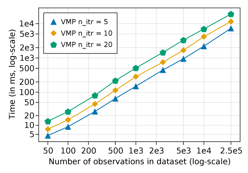
The main benchmark results are presented in Table 4. Fig. 13 presents a comparison of the performance of the ReactiveMP.jl as a function of the number of VMP iterations and shows that the resulting inference procedure scales linearly both on the number of observations and the number of VMP iterations performed. In the context of VMP, each iteration decreases the Bethe Free and effectively leads to a better approximation for the marginals over the latent variables. As in our previous example, we show the accuracy results for message passing-based methods in comparison with sampling-based methods in terms of metric (12) in Table 5. The ForneyLab.jl shows the same level of posterior accuracy, as it uses the same VMP algorithm, but is slower in model compilation and execution times. The Turing.jl is set to use the HMC method for estimating the posterior of transition matrices and with a combination of particle Gibbs (PG) for discrete states .
| Number of observations | ||||
| Package | 100 | 250 | 10 000 | 25 000 |
| ReactiveMP.jl | 21 | 62 | 5624 | 15544 |
| ForneyLab.jl (compilation) | 82280 | 405949 | - | - |
| ForneyLab.jl (inference) | 93 | 228 | - | - |
| Turing.jl HMC+PG (250) | 93956 | 396946 | - | - |
| Turing.jl HMC+PG (500) | 186293 | 783850 | - | - |
| Number of observations | |||
|---|---|---|---|
| Method | 50 | 100 | 250 |
| Message passing | 0.10 | 0.09 | 0.07 |
| HMC+PG (250) | 0.50 | 0.51 | 0.52 |
| HMC+PG (500) | 0.51 | 0.49 | 0.51 |

6.3 Hierarchical Gaussian Filter
For our last example, we consider Bayesian inference in the Hierarchical Gaussian Filter (HGF) model. The HGF is popular in the computational neuroscience literature and is often used for the Bayesian modelling of volatile environments, such as uncertainty in perception or financial data (Mathys et al., 2014). The HGF is essentially a Gaussian random walk, where the time-varying variance of the random walk is determined by the state of a higher level process, e.g., a Gaussian random walk with fixed volatily or another more complex signal. Specifically, a simple HGF is defined as
| (17a) | ||||
| (17b) | ||||
where is the observation at time step , is the latent state for the -th layer at time step , and is a link function, which maps states from the (next higher) layer to the non-negative variance of the random walk in the -th layer. The HGF model typically defines the link function as , where and are either hyper-parameters or random variables included in the model.
As in the previous example, the exact Bayesian inference for this type of model is not tractable. Moreover, the variational message update rules (9) are not tractable either since the HGF model contains non-conjugate relationships between variables in the form of the link function . However, inference in this model is still possible with custom message update rules approximation (Senoz and De Vries, 2018). The ReactiveMP.jl package supports a straightforward API to add custom nodes with custom message passing update rules. In fact, a big part of the ReactiveMP.jl library is a collection of well-known factor nodes and message update rules implemented using the same API as for custom novel nodes and message update equations. The API also supports message update rules that involve extra nontrivial approximation steps. In this example, we added a custom Gaussian controlled variance (GCV) node to model the nonlinear time-varying variance mapping from different hierarchy levels (17a), with a set of approximate update rules based on the Gauss-Hermite cubature rule from (Kokkala et al., 2015). The main purpose of this example is to show that ReactiveMP.jl is capable of running inference in complex non-conjugate models, but requires creating custom factor nodes and choosing appropriate integral calculation approximation methods.
CBFE Specification
In this example, we want to show an example of reactive online Bayesian learning (filtering) in a 2-layer HGF model. For simplicity and to avoid extra clutter, we assume , and to be fixed, but there are no principled limitations to make them random variables, endow them with priors and to estimate their corresponding posterior distributions. For online learning in the HGF model (17) we define only a single time step and specify the structured factorisation assumption for state transition nodes as well as for higher layer random walk transition nodes and the mean-field assumption for other functional dependencies in the model:
| (18a) | ||||
| (18b) | ||||
| (18c) | ||||
We show an example of a HGF model specification in Listing 10. For the approximation of the integral in the message update rule, the GCV node requires a suitable approximation method to be specified during model creation. For this reason we create a metadata object called GCVMetadata() that accepts a GaussHermiteCubature() approximation method with a prespecified number of sigma points gh_n.
Inference
For the inference procedure, we adopt the technique from the Infinite Recursive Chain Processing section (Section 4.2.5). We subscribe to future observations, perform a prespecified number of VMP iterations for each new data point, and redirect the last posterior update as a prior for the next future observation. The resulting inference procedure reacts to new observations autonomously and is compatible with infinite data streams. We show a part of the inference procedure for the model (17) in Listing 11. Full code is available at GitHub experiment’s repository.


We show the inference results in Fig. 14. Fig. 14(c) shows convergence of the Bethe Free Energy after several number of VMP iterations. Qualitative results in Fig. 14(a) and in Fig. 14(b) show correct posterior estimation of continuously valued hidden states even though the model contains non-conjugate relationships between variables.
Benchmark
The main benchmark results are presented in Table 6 and accuracy comparison in Table 7. We show the performance of the ReactiveMP.jl package depending on the number of observations and the number of VMP iterations for this particular model in Fig. 15. As in the previous example, we note that that the ReactiveMP.jl framework scales linearly both with the number of observations and with the number of VMP iterations performed.
| Number of observations | |||||
| Package | 50 | 100 | 250 | 10 000 | 100 000 |
| ReactiveMP.jl | 19 | 38 | 95 | 4412 | 45889 |
| ForneyLab.jl (compilation) | 590 | 582 | 592 | - | - |
| ForneyLab.jl (inference) | 457 | 876 | 2368 | - | - |
| Turing.jl (500) | 1357 | 2607 | 6531 | - | - |
| Turing.jl (1000) | 3036 | 5287 | 12847 | - | - |
| Number of observations | ||||||
| layer | layer | |||||
| Method | 50 | 100 | 250 | 50 | 100 | 250 |
| Message passing | 0.89 | 0.79 | 0.75 | 0.36 | 0.35 | 0.35 |
| HMC (500) | 1.41 | 1.29 | 1.51 | 0.45 | 0.62 | 4.74 |
| HMC (1000) | 1.30 | 1.14 | 1.22 | 0.41 | 0.49 | 2.56 |
We can see that, in contrast with previous examples where we performed inference on a full graph, the ForneyLab.jl compilation time is not longer dependent on the number of observations and the model compilation is more acceptable due to the fact that we always build a single time step of a graph and reuse it during online learning. Both the ReactiveMP.jl and ForneyLab.jl show the same scalability and posterior accuracy results as they both use the same method for posterior approximation, however, ReactiveMP.jl is faster in VMP inference execution in absolute timing.
In this model, the HMC algorithm shows less accurate results in terms of the metric (12). However, because of the online learning setting, the model has a small number of unknowns, which makes the HMC algorithm more feasible to perform inference for a large number of observations in comparison with the previous examples. The advantage of using Turing.jl is that it supports inference for non-conjugate relationships between variables in a model by default, and, hence, does not require hand-crafted custom factor nodes and message update rule approximations.


7 Discussion
We are investigating several possible future directions for the reactive message passing framework that could improve its usability and performance. We believe that the current implementation is efficient and flexible enough to perform real-time reactive Bayesian inference and has been tested on both synthetic and real data sets. The new framework allows for large models to be applied in practice and simplifies the model exploration process in signal processing applications. A natural future direction is to apply the new framework to an Active Inference (Friston et al., 2016) setting. A reactive active inference agent learns purposeful behavior solely through situated interactions with its environment and processing these interactions by real-time inference. As we discussed in the Motivation (Section 2), an important issue for autonomous agents is robustness of the running Bayesian inference processes, even when nodes or edges collapse under situated conditions. ReactiveMP.jl supports in-place model adjustments during the inference procedure as well as handles missing data observations, but it does not export any user-friendly API yet. For the next release of our framework, we aim to export a public API for robust Bayesian inference to simplify the development of Active Inference agents. In addition, our plan is to proceed with further optimisation of the current implementation and improve the scalability of the existing package in real-time on embedded devices. Moreover, the Julia programming language is developing and improving, thus we expect it to be even more efficient in the coming years.
Reactive programming allows us to easily integrate additional features into our new framework. First, we are investigating the possibility to run reactive message passing-based inference in parallel on multiple CPU cores (Särkkä and García-Fernández, 2020). RP does not make any assumptions in the underlying data generation process and does not distinguish synchronous and asynchronous data streams. Secondly, reactive systems allow us to integrate local stopping criteria for passing messages. In some scenarios, we may want to stop passing messages based on some pre-specified criterion and simply stop reacting to new observations and save battery life on a portable device or to save computational power for other tasks. Thirdly, our current implementation does not provide extensive debugging tools yet, but it might be crucial to analyse the performance of message passing-based methods step-by-step. We are looking into options to extend the graphical notation and integrate useful debug methods with the new framework to analyze and debug message passing-based inference algorithms visually in real-time and explore their performance characteristics. Since the ReactiveMP.jl package uses reactive observables under the hood, it should be straightforward to ‘‘spy’’ on all updates in the model for later or even real-time performance analysis. That should even further simplify the process of model specification as one may change the model in real-time and immediately see the results.
Moreover, we are in a preliminary stage of extending the set of available message passing rules to non-conjugate prior and likelihood pairs (Akbayrak and Bocharov, 2021). The generic probabilistic toolboxes in the Julia language like Turing.jl support inference in a broader range of probabilistic models, which is currently not the case for the ReactiveMP.jl. We are working on future message update rules extension and potential integration with other probabilistic frameworks in the Julia community.
Finally, another interesting future research direction is to decouple the model specification language from the factorisation and the form constraint specification on a variational family of distributions . This would allow to have a single model and a set of constrained variational families of distributions so we could run and compare different optimisation procedures and their performance simultaneously or trade off computational complexity with accuracy in real-time.
8 Conclusions
In this paper, we presented methods and implementation aspects of a reactive message passing (RMP) framework both for exact and approximate Bayesian inference, based on minimization of a constrained Bethe Free Energy functional. The framework is capable of running hybrid algorithms with BP, EP, EM, and VMP analytical message update rules and supports local factorisation as well as form constraints on the variational family. We implemented an efficient proof-of-concept of RMP in the form of the ReactiveMP.jl package for the Julia programming language, which exports an API for running reactive Bayesian inference, and scales easily to large state space models with hundreds of thousands of unknowns. The inference engine is highly customisable through ad hoc construction of custom nodes, message update rules, approximation methods, and optional modifications to the default computational pipeline. Experimental results for a set of various standard signal processing models showed better performance in comparison to other existing Julia packages and sampling-based methods for Bayesian inference. We believe that the reactive programming approach to message passing-based methods opens a lot of directions for further research and will bring real-time Bayesian inference closer to real-world applications.
Acknowledgement
We would like to acknowledge the assistance and their contributions to the source code of the ReactiveMP.jl package from Ismail Senoz, Albert Podusenko, and Bart van Erp. We acknowledge the support and helpful discussions from Thijs van de Laar - one of the creators of the ForneyLab.jl package. We are also grateful to all BIASlab team members for their support during the early stages of the development of this project.
References
- Martín Abadi et al. [2015] Martín Abadi, Ashish Agarwal, Paul Barham, Eugene Brevdo, Zhifeng Chen, Craig Citro, Greg S. Corrado, Andy Davis, Jeffrey Dean, Matthieu Devin, Sanjay Ghemawat, Ian Goodfellow, Andrew Harp, Geoffrey Irving, Michael Isard, Yangqing Jia, Rafal Jozefowicz, Lukasz Kaiser, Manjunath Kudlur, Josh Levenberg, Dandelion Mané, Rajat Monga, Sherry Moore, Derek Murray, Chris Olah, Mike Schuster, Jonathon Shlens, Benoit Steiner, Ilya Sutskever, Kunal Talwar, Paul Tucker, Vincent Vanhoucke, Vijay Vasudevan, Fernanda Viégas, Oriol Vinyals, Pete Warden, Martin Wattenberg, Martin Wicke, Yuan Yu, and Xiaoqiang Zheng. TensorFlow: Large-Scale Machine Learning on Heterogeneous Systems, 2015. URL https://www.tensorflow.org/.
- Paszke et al. [2019] Adam Paszke, Sam Gross, Francisco Massa, Adam Lerer, James Bradbury, Gregory Chanan, Trevor Killeen, Zeming Lin, Natalia Gimelshein, Luca Antiga, Alban Desmaison, Andreas Kopf, Edward Yang, Zachary DeVito, Martin Raison, Alykhan Tejani, Sasank Chilamkurthy, Benoit Steiner, Lu Fang, Junjie Bai, and Soumith Chintala. PyTorch: An Imperative Style, High-Performance Deep Learning Library. In H. Wallach, H. Larochelle, A. Beygelzimer, F. d’ Alché-Buc, E. Fox, and R. Garnett, editors, Advances in Neural Information Processing Systems 32, pages 8024--8035. Curran Associates, Inc., 2019. URL http://papers.neurips.cc/paper/9015-pytorch-an-imperative-style-high-performance-deep-learning-library.pdf.
- Friston [2009] Karl Friston. The free-energy principle: a rough guide to the brain? Trends in Cognitive Sciences, 13(7):293--301, July 2009. ISSN 13646613. doi:10.1016/j.tics.2009.04.005. URL http://linkinghub.elsevier.com/retrieve/pii/S136466130900117X.
- van de Laar et al. [2018] Thijs van de Laar, Marco Cox, and Bert de Vries. ForneyLab.jl: a Julia Toolbox for Factor Graph-based Probabilistic Programming. In JuliaCon, London, UK, August 2018.
- Minka et al. [2018] T. Minka, J.M. Winn, J.P. Guiver, Y. Zaykov, D. Fabian, and J. Bronskill. /Infer.NET 0.3, 2018.
- Elidan et al. [2012] Gal Elidan, Ian McGraw, and Daphne Koller. Residual Belief Propagation: Informed Scheduling for Asynchronous Message Passing. arXiv:1206.6837 [cs], June 2012. URL http://arxiv.org/abs/1206.6837. arXiv: 1206.6837.
- Bishop [2006] Christopher M. Bishop. Pattern Recognition and Machine Learning. Springer-Verlag New York, Inc., 2006. ISBN 0-387-31073-8. URL http://www.springer.com/computer/image+processing/book/978-0-387-31073-2.
- Boussinot et al. [2015] Frédéric Boussinot, Bernard Monasse, and Jean-Ferdy Susini. Reactive Programming of Simulations in Physics. International Journal of Modern Physics C, 26(12):1550132, December 2015. ISSN 0129-1831, 1793-6586. doi:10.1142/S0129183115501326. URL http://arxiv.org/abs/1410.7763. arXiv: 1410.7763.
- Busch et al. [2020] Julian Busch, Jiaxing Pi, and Thomas Seidl. PushNet: Efficient and Adaptive Neural Message Passing. arXiv:2003.02228 [cs, stat], December 2020. doi:10.3233/FAIA200199. URL http://arxiv.org/abs/2003.02228. arXiv: 2003.02228.
- Baudart et al. [2019] Guillaume Baudart, Louis Mandel, Eric Atkinson, Benjamin Sherman, Marc Pouzet, and Michael Carbin. Reactive Probabilistic Programming. August 2019. URL https://arxiv.org/abs/1908.07563v1.
- Forney [2001] G.David Forney. Codes on graphs: normal realizations. IEEE Transactions on Information Theory, 47(2):520--548, February 2001. ISSN 0018-9448. doi:10.1109/18.910573. URL https://ieeexplore.ieee.org/abstract/document/910573.
- Loeliger [2004] Hans-Andrea Loeliger. An introduction to factor graphs. Signal Processing Magazine, IEEE, 21(1):28--41, January 2004. doi:10.1109/MSP.2004.1267047. URL https://ieeexplore.ieee.org/document/1267047.
- Korl [2005] Sascha Korl. A factor graph approach to signal modelling, system identification and filtering. PhD thesis, Swiss Federal Institute of Technology, Zurich, 2005.
- Winn [2003] John Winn. Variational message passing and its applications. PhD thesis, 2003. URL http://johnwinn.org/Publications/thesis/Winn03_thesis.pdf.
- Dauwels [2007] Justin Dauwels. On Variational Message Passing on Factor Graphs. In IEEE International Symposium on Information Theory, pages 2546--2550, Nice, France, June 2007. doi:10.1109/ISIT.2007.4557602. URL http://ieeexplore.ieee.org/abstract/document/4557602.
- Şenöz et al. [2021] İsmail Şenöz, Thijs van de Laar, Dmitry Bagaev, and Bert de Vries. Variational Message Passing and Local Constraint Manipulation in Factor Graphs. Entropy, 23(7):807, 2021. doi:10.3390/e23070807. Publisher: Multidisciplinary Digital Publishing Institute.
- Yedidia et al. [2001] Jonathan S Yedidia, William T Freeman, and Yair Weiss. Bethe free energy, Kikuchi approximations, and belief propagation algorithms. Advances in neural information processing systems, 13:24, 2001.
- Yedidia et al. [2005] Jonathan S. Yedidia, W.T. Freeman, and Y. Weiss. Constructing free-energy approximations and generalized belief propagation algorithms. IEEE Transactions on Information Theory, 51(7):2282--2312, July 2005. ISSN 0018-9448. doi:10.1109/TIT.2005.850085. URL http://ieeexplore.ieee.org/abstract/document/1459044.
- Zhang et al. [2017] Dan Zhang, Wenjin Wang, Gerhard Fettweis, and Xiqi Gao. Unifying Message Passing Algorithms Under the Framework of Constrained Bethe Free Energy Minimization. arXiv:1703.10932 [cs, math], March 2017. URL http://arxiv.org/abs/1703.10932. arXiv: 1703.10932.
- Akbayrak and de Vries [2019] Semih Akbayrak and Bert de Vries. Reparameterization Gradient Message Passing. In submitted to EUSIPCO, page 5, 2019.
- Raymond et al. [2014] Jack Raymond, Andre Manoel, and Manfred Opper. Expectation Propagation. arXiv preprint arXiv:1409.6179, 2014. URL http://arxiv.org/abs/1409.6179.
- Cox [2018] Marco Cox. Robust Expectation Propagation in Factor Graphs Involving Both Continuous and Binary Variables. In 26th European Signal Processing Conference (EUSIPCO), page 5, Rome, Italy, 2018.
- Bezanson et al. [2017] J. Bezanson, A. Edelman, S. Karpinski, and V. Shah. Julia: A Fresh Approach to Numerical Computing. SIAM Review, 59(1):65--98, January 2017. ISSN 0036-1445. doi:10.1137/141000671. URL https://epubs.siam.org/doi/abs/10.1137/141000671.
- Besançon et al. [2021] Mathieu Besançon, Theodore Papamarkou, David Anthoff, Alex Arslan, Simon Byrne, Dahua Lin, and John Pearson. Distributions.jl: Definition and Modeling of Probability Distributions in the JuliaStats Ecosystem. Journal of Statistical Software, 98(16):1--30, 2021. ISSN 1548-7660. doi:10.18637/jss.v098.i16. URL https://www.jstatsoft.org/v098/i16.
- Lin et al. [2019] Dahua Lin, John Myles White, Simon Byrne, Douglas Bates, Andreas Noack, John Pearson, Alex Arslan, Kevin Squire, David Anthoff, Theodore Papamarkou, Mathieu Besançon, Jan Drugowitsch, Moritz Schauer, and other contributors. JuliaStats/Distributions.jl: a Julia package for probability distributions and associated functions, July 2019. URL https://doi.org/10.5281/zenodo.2647458.
- Podusenko et al. [2021] Albert Podusenko, Bart van Erp, Dmitry Bagaev, Ismail Senoz, and Bert de Vries. Message Passing-Based Inference in the Gamma Mixture Model. In 2021 IEEE 31st International Workshop on Machine Learning for Signal Processing (MLSP), pages 1--6, Gold Coast, Australia, October 2021. IEEE. ISBN 978-1-72816-338-3. doi:10.1109/MLSP52302.2021.9596329. URL https://ieeexplore.ieee.org/document/9596329/.
- van Erp et al. [2021] Bart van Erp, Albert Podusenko, Tanya Ignatenko, and Bert de Vries. A Bayesian Modeling Approach to Situated Design of Personalized Soundscaping Algorithms. Applied Sciences, 11(20):9535, October 2021. doi:10.3390/app11209535. URL https://www.mdpi.com/2076-3417/11/20/9535. Number: 20 Publisher: Multidisciplinary Digital Publishing Institute.
- Podusenko et al. [2022] Albert Podusenko, Bart van Erp, Magnus Koudahl, and Bert de Vries. AIDA: An Active Inference-based Design Agent for Audio Processing Algorithms. 2022. In preparation.
- Ge et al. [2018] Hong Ge, Kai Xu, and Zoubin Ghahramani. Turing: A Language for Flexible Probabilistic Inference. In International Conference on Artificial Intelligence and Statistics, pages 1682--1690, March 2018. URL http://proceedings.mlr.press/v84/ge18b.html. ISSN: 1938-7228 Section: Machine Learning.
- Chen and Revels [2016] Jiahao Chen and Jarrett Revels. Robust benchmarking in noisy environments. arXiv e-prints, August 2016. _eprint: 1608.04295.
- Sarkka [2013] Simo Sarkka. Bayesian Filtering and Smoothing. Cambridge University Press, New York, NY, USA, 2013. ISBN 978-1-107-61928-9.
- Särkkä [2008] Simo Särkkä. Unscented Rauch–Tung–Striebel Smoother. IEEE Transactions on Automatic Control, 53(3):845--849, 2008.
- Jelinek [1998] Frederick Jelinek. Statistical Methods for Speech Recognition. MIT Press, Cambridge, MA, USA, 1998. ISBN 0-262-10066-5.
- Rabiner and Juang [1993] Lawrence R. Rabiner and B. H. Juang. Fundamentals of speech recognition. Prentice Hall signal processing series. PTR Prentice Hall, Englewood Cliffs, N.J, 1993. ISBN 978-0-13-015157-5.
- Manning and Schütze [1999] Christopher D. Manning and Hinrich Schütze. Foundations of Statistical Natural Language Processing. The MIT Press, Cambridge, Massachusetts, 1999. URL http://nlp.stanford.edu/fsnlp/.
- Zhang et al. [2014] Zhihua Zhang, Dakan Wang, Guang Dai, and Michael I. Jordan. Matrix-Variate Dirichlet Process Priors with Applications. Bayesian Analysis, 9(2):259 -- 286, 2014. doi:10.1214/13-BA853. URL https://doi.org/10.1214/13-BA853. Publisher: International Society for Bayesian Analysis.
- Mathys et al. [2014] Christoph D. Mathys, Ekaterina I. Lomakina, Jean Daunizeau, Sandra Iglesias, Kay H. Brodersen, Karl J. Friston, and Klaas E. Stephan. Uncertainty in perception and the Hierarchical Gaussian Filter. Frontiers in Human Neuroscience, 8, November 2014. ISSN 1662-5161. doi:10.3389/fnhum.2014.00825. URL https://www.ncbi.nlm.nih.gov/pmc/articles/PMC4237059/.
- Senoz and De Vries [2018] Ismail Senoz and Bert De Vries. Online State and Parameter Estimation in the Hieararchical Gaussian Filter. 2018 IEEE International Workshop on Machine Learning for Signal Processing, MLSP 2018 - Proceedings, September 2018.
- Kokkala et al. [2015] Juho Kokkala, Arno Solin, and Simo Särkkä. Sigma-Point Filtering and Smoothing Based Parameter Estimation in Nonlinear Dynamic Systems. arXiv:1504.06173 [math, stat], November 2015. URL http://arxiv.org/abs/1504.06173. arXiv: 1504.06173.
- Friston et al. [2016] Karl Friston, Thomas FitzGerald, Francesco Rigoli, Philipp Schwartenbeck, John O’Doherty, and Giovanni Pezzulo. Active inference and learning. Neuroscience & Biobehavioral Reviews, 2016. ISSN 0149-7634. doi:10.1016/j.neubiorev.2016.06.022. URL http://www.sciencedirect.com/science/article/pii/S0149763416301336.
- Särkkä and García-Fernández [2020] Simo Särkkä and Ángel F. García-Fernández. Temporal Parallelization of Bayesian Smoothers. arXiv:1905.13002 [cs, math, stat], February 2020. URL http://arxiv.org/abs/1905.13002. arXiv: 1905.13002.
- Akbayrak and Bocharov [2021] Semih Akbayrak and Ivan Bocharov. Extended Variational Message Passing for Automated Approximate Bayesian Inference. page 34, 2021.