Re-examining aggregation in the Tallis-Leyton model of parasite acquisition
Abstract.
The Tallis-Leyton model is a simple model of parasite acquisition where there is no interaction between the host and the acquired parasites. We examine the effect of model parameters on the distribution of the host’s parasite burden in the sense of the Lorenz order. This fits with an alternate view of parasite aggregation that has become widely used in empirical studies but is rarely used in the analysis of mathematical models of parasite acquisition.
1. Introduction
The distribution of parasites among its host population typically displays a high degree of inequality. In fact, this phenomenon, called aggregation, is almost a universally observed (Shaw and Dobson, 1995, Poulin, 2007). Despite its importance, aggregation lacks a universally accepted definition. Instead, the phenomenon is studied using a number of common measures of aggregation that summarise different properties of the parasite’s distribution (Pielou, 1977, McVinish and Lester, 2020, Morrill et al., 2023). The most commonly used measures of aggregation in theoretical models are the parameter of the negative binomial distribution (Anderson and May, 1978a, b, Rosa and Pugliese, 2002, Schreiber, 2006, McPherson et al., 2012) and the variance-to-mean ratio (Isham, 1995, Barbour and Pugliese, 2000, Herbert and Isham, 2000, Peacock et al., 2018). Both of these measures can be interpreted as quantifying how far the distribution of parasites deviates from a Poisson distribution.
An alternative view of aggregation was put forward by Poulin (1993), arguing that a measure of the discrepancy between the observed distribution of parasites in the hosts and the ideal distributions where all hosts are infected with the same number of parasites would be the best measure of aggregation. This view puts the Lorenz ordering of distributions (Lorenz, 1905, Arnold and Sarabia, 2018) central in the study of aggregation. As a measure of this discrepancy, Poulin proposed his index, D, which is essentially an estimator of the Gini index (Gini, 1924). This has since become become one of the standard measure of aggregation used in studies of wild parasite populations. Although the Gini index has been commonly used in empirical studies since Poulin’s proposal, we are unaware of any examination of its behaviour in theoretical models of parasite acquisition.
The aim of this paper is to apply Poulin’s view of aggregation to a simple stochastic model for the number of parasites in a definitive host proposed by Tallis and Leyton (1969). The Tallis-Leyton model assumes that the host makes infective contacts following a Poisson process and at each infective contact a random number of parasites enter the host. Once a parasite enters the host, it is alive for a random period of time. The lifetimes of parasites, numbers of parasites entering the host at infective contacts, and the Poisson process of infective contacts are all assumed to be independent. Furthermore, the parasites are assumed to have no effect on the host mortality.
In Section 2 we review some background on the Lorenz ordering and the closely related convex ordering of distributions. The Tallis-Leyton model is analysed in Section 3. We first show show how the host’s parasite burden can be represented as a compound Poisson distribution. This representation is then applied to determine how each of the model parameters affect the Lorenz ordering of the distribution of parasites in the host. The final part of the analysis shows that the host’s parasite burden is asymptotically normally distributed in the limit as the rate of infectious contacts goes to infinity. The paper concludes with a discussion of future challenges in analysing models of parasite aggregation.
2. Background
2.1. Tallis-Leyton model
Tallis and Leyton (1969) proposed the following model for the parasite burden of a definitive host at age , conditional on survival of the host to age . The host is assumed to be parasite free at birth so . The host makes infective contacts during its lifetime following a Poisson process with rate parameter . At each infective contact, the number of parasites that enter the host is a random variable and once a parasite enters the host it survives for a random period . The parasites have no effect on the host mortality. The lifetimes of parasites, numbers of parasites entering the host at infective contacts, and the Poisson process of infective contacts are all assumed to be independent. Although we won’t make use of this fact, we note that this process also describes an infinite server queue with bulk arrivals and general independent service times (Holman et al., 1983).
We let , and denote the probability generating function (PGF), distribution function, and survival function of a random variable . We write for the PGF of , conditional on survival of the host to age . Tallis and Leyton (1969) showed
Standard arguments show that the mean and variance of are
Hence, the variance-to-mean ratio is
| (1) |
Assuming and , the limiting distribution of parasite burden as exists and has PGF
Since scaling of the host age, the lifetime distribution of parasites, and the inverse of the rate of infective contacts by a common factor results in the same distribution for the host’s parasite burden, we assume that the expected lifetime of a parasite is 1.
2.2. Convex order and Lorenz order
Lorenz (1905) proposed the Lorenz curve as a graphical measure of inequality. The following general definition of the Lorenz curve was given by Gastwirth (1971).
Definition.
The Lorenz curve for the distribution with finite mean is given by
where is the quantile function
Adapting the description in Arnold and Sarabia (2018, Section 3.1) to a parasitology context, the Lorenz curve represents the proportion of the parasite population infecting the least infected proportion of the host population. When all hosts are infected with the same number of parasite, the Lorenz curve is given by and is called the egalitarian line. Note that for all .
The Lorenz curve defines a partial order on the class of all distributions on with finite mean (Arnold and Sarabia, 2018, Definition 3.2.1).
Definition.
Let and be random variables with the respective Lorenz curves denoted and . We say is smaller in the Lorenz order, denoted if for every .
The Lorenz curves of some standard distributions are given in Arnold and Sarabia (2018, Section 6.1). The negative binomial distribution is extensively used in parasitology. When negative binomial distributions are parameterised in terms of the mean and , they can be compared in the Lorenz order (McVinish and Lester, 2024). Specifically, let denote the negative binomial distribution with PGF
Then
-
(i)
for any and , , and
-
(ii)
for any and , .
Closely related to the Lorenz order is the convex order of distributions.
Definition.
Let and be two random variables such that . We say is small than in the convex order, denoted , if for all convex functions , provided the expectations exist.
These two orderings are related since if and only if
for every continuous convex function (Arnold and Sarabia, 2018, Corollary 3.2.1). In other words,
| is equivalent to |
Shaked and Shanthikumar (2007, Section 3.A) provide an extensive review of results on the convex order. We briefly mention some of the important results that are used in our analysis.
-
•
The convex order is closed under weak limits provided the expectations also converge (Shaked and Shanthikumar, 2007, Theorem 3.A.12 (c)).
-
•
The convex order is closed under mixtures (Shaked and Shanthikumar, 2007, Theorem 3.A.12 (b)). Let , , and be random variables and write and for the conditional distributions of and given . If for all in the support of , then . As an application of this property we can say that if and is an independent non-negative random variable, then .
-
•
The convex order is closed under convolutions (Shaked and Shanthikumar, 2007, Theorem 3.A.12 (d)). Let and be two sets of independent random variables . If for , then
-
•
Combining the properties of closure under mixtures and closure under convolutions, we see the convex order is closed under random sums so
for any non-negative integer random variable . As an application of the closure under random sums property of the convex order, consider two random variables and that related by binomial thinning. That is, for some . Then (McVinish and Lester, 2020, Section 3)
-
•
The closure under random sums property can be adapted to the case where the and are two iid sequences with , and and are non-negative integer random variables such that . In this case, Shaked and Shanthikumar (2007, Theorem 3.A.13) implies
-
•
The survival function can be used to establish if two random variables can be compared in the convex order. If and are two random variables with the same mean, then if has a single sign change and the sign sequence is (Shaked and Shanthikumar, 2007, Theorem 3.A.44(b)). This property can also be used to characterise the convex order (Shaked and Shanthikumar, 2007, Theorem 3.A.45).
2.3. Measures of aggregation
In practice, levels of aggregation are compared with numerical summaries rather than using the entire Lorenz curve. A useful measure of aggregation respects the Lorenz ordering. That is, if is a measure of aggregation that respects the Lorenz ordering and , then . Arnold and Sarabia (2018, Chapter 5) review several inequality measures and these can be applied as measures of aggregation. We restrict our attention in this paper to the Gini index, the Hoover index (also known as the Pietra index, or the Robin-Hood index), , and the coefficient of variation.
The Gini index (Gini, 1924) is given by twice the area between the egalitarian line and the Lorenz curve. For a random variable , the Gini index can be expressed as
where is an independent random variable with . The Hoover index is given by the maximum vertical distance between the egalitarian line and the Lorenz curve. McVinish and Lester (2020) argue that this index could be useful due to its simple interpretation as the proportion of the parasite population that would need to be redistributed among the hosts in order for all hosts to have the same parasite burden. The Hoover index can be expressed as
Prevalence, the probability that a host is infected by at least one parasite, is an important quantity in parasitology. Although prevalence is not usually thought of as a measure of aggregation, we may express in terms of the Lorenz curve as
For the Tallis-Leyton model,
| (2) |
Finally, the coefficient of variation is given by
This measure is rarely used in parasitology, though it is mentioned in some reviews on parasite aggregation such as Wilson et al. (2001) and McVinish and Lester (2020). As means and variances are commonly reported in empirical studies and are often easily calculated for theoretical models, it may be useful in some contexts. For example, the squared coefficient of variation for the Tallis-Leyton model is
| (3) |
These indices are related by the following inequality
(Taguchi, 1968, McVinish and Lester, 2020). In particular, if , then we have the equality . The Gini index and Hoover index can be further related to the coefficient of variation when the distribution of parasites is approximately normal. Suppose is a sequence of random variables such that
where . As with probability one, the above limit is only possible if . Nevertheless, the ratio of the Hoover index to the coefficient of variation still has a well defined limit. The Hoover index of can be expressed as
Since , this collection of random variables is uniformly integrable and . Hence,
| (4) |
Similarly, the Gini index of can be expressed as
where is an independent random variable with . Applying the asymptotic normality and uniform integrability of the ,
| (5) |
2.4. Numerical evaluation
From equation (3), the coefficient of variation can be relatively easily evaluated for the Tallis-Leyton model. Numerical integration of and may be required, but the dependence on age and is explicit. Similarly, could be evaluated with a single numerical integration using (2). On the other hand, evaluation of the Hoover and Gini indices require evaluation of the probability mass function. In the examples of the next section, we numerically evaluate the probability mass function of by inverting using the Abate-Whitte algorithm (Abate and Whitt, 1992). The algorithm was implemented in MATLAB (The MathWorks Inc., 2022a) using the vpa function in the Symbolic Math Toolbox (The MathWorks Inc., 2022b) for high precision arithmetic.
3. Analysis of the Tallis-Leyton model
The analysis begins with a representation of the host’s parasite burden as a compound Poisson distribution. This representation is used extensively to understand how the rate of infective contacts, the distribution of the number of parasites that enter the host during an infective contact, the age of the host, and lifetime distribution of the parasites all affect the distribution of parasites in the host in terms of the Lorenz order. When comparing the host’s parasite burden in two systems, the parameters of the second parasite-host system is distinguished by a tilde.
3.1. Compound Poisson representation
Let be a sequence of independent standard uniform random variables and define by
with when . For given and the distribution of is .
Theorem 1.
Assume has a continuous distribution. Define to be a random variable on with distribution function
| (6) |
Let be a sequence of independent random variables with the same distribution as , where and are independent. Let be a Poisson process with rate so . Then
Proof.
Standard conditioning arguments show that the PGF of is
Hence,
Again applying standard conditioning arguments, we see the PGF of is
Upon making the substitution , the PGF of can be expressed as
∎
3.2. Rate of infective contacts
Our first comparison result concerns the effect of the rate of infective contacts on the distribution of the host’s parasite burden. The rate of infective contacts has no effect on the variance-to-mean ratio (1), whereas the coefficient of variation is strictly decreasing as the rate of infective contacts increases (3). The following result shows that any index respecting the Lorenz order is decreasing as a function of the rate of infective contacts.
Theorem 2.
If and all other model parameters are equal, then .
Proof.
Set . Let be a sequence of independent random variables having the same distribution as and let be a sequence of independent random variables that are also independent of the . As and the convex order is closed under mixtures, . The PGF of is . Let be a Poisson process with rate . As the convex order is closed under random sums,
By Theorem 1, . To determine the distribution of , we evaluate its PGF
Hence, . ∎
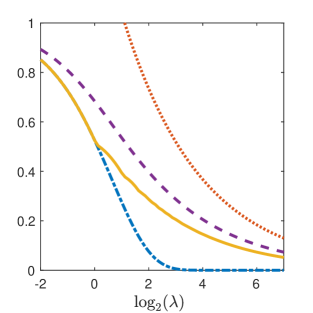
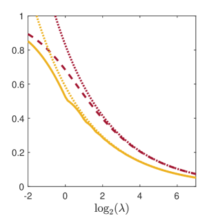
Figure 1 shows the four indices (Gini, Hoover, , and coefficient of variation) for a host aged 3 where , , and . Since the coefficient of variation (3) is proportional to , it is not displayed for small values of . We see that all four indices are strictly decreasing as a function of . For , so the Hoover index and . The Hoover index appears to display some discontinuity in the first derivative at points where the expectation is integer valued. This behaviour is less apparent at larger values of .
3.3. Distribution of
We now consider the role of the distribution of the number of parasites that enter the host during an infective contact. As a concrete example, suppose . Then the variance-to-mean ratio is
where is a constant depending on . From this expression we see that the variance-to-mean ratio is increasing in but decreasing in . In contrast, the coefficient of variation of is decreasing in both and . The next two results show that the distribution of the host’s parasite burden is decreasing in the Lorenz order as functions of both and . The first of these results requires the distributions being compared to have the same expectation.
Theorem 3.
Suppose and all other model parameters are equal. Then .
Proof.
Using an extension of the closure under random sums property of the convex order Shaked and Shanthikumar (2007, Theorem 3.A.13),
As the convex order is closed under mixtures, . Let be a sequence of independent random variables having the same distribution as and let be a sequence of independent random variables having the same distribution as . As the convex order is closed under random sums,
Theorem 1 shows . ∎
For distributions with different means, we consider only the case where and are related by binomial thinning. Recall that if for some , then .
Theorem 4.
Suppose that for some and all other model parameters are equal. Then .
Proof.
Let and be independent standard uniform random variables. Then standard conditioning arguments show
As the convex order is closed under mixtures,
As the convex order is closed under random sums, . Following the same arguments as in the proof of Theorem 3, we see . Hence, . ∎
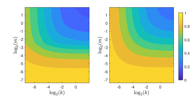
As noted previously, if and . If , and all other model parameters are equal, then Theorems 3 and 4 together imply that . Figure 2 shows the Hoover and Gini indices as functions of the negative binomial parameters and for a parasite host system with host aged 10, rate of infective contacts 5, and parasite lifetimes following an exponential distribution with mean 1. Both indices are decreasing in both and as we expect from the above results. The contours of the Hoover index display some discontinuity in the first derivative for (), which corresponds to a mean of 1 for the host. The contours for both the Hoover and Gini indices tend to become parallel to the respective axes as and . This is a consequence of the limiting behaviour of the negative binomial distribution (Adell and Cal, 1994).
It is natural to consider which distribution for results in the least aggregated distribution for the host’s parasite burden. This requires determining the smallest distribution in the convex ordering. The convex order requires that the distributions compared have the same expected value so let . Define the random variable such that
In the supplementary material of McVinish and Lester (2020) it was shown that so is smallest distribution in convex order with expectation . When , the smallest distribution in convex order for leads to having a Poisson distribution. There is no largest distribution in the convex order.
3.4. Host age
Differentiating (1) with respect to age shows the variance-to-mean ratio is a decreasing function of age. Since the expected parasite burden is increasing in age, the coefficient of variation is also decreasing in age. The following result shows the host’s parasite burden is decreasing in the Lorenz order as a function of age.
Theorem 5.
If , then .
The proof is built from the following lemmas.
Lemma 6.
Proof.
Note that
so . We show that by examining the sign changes of . The survival functions of and are
and
Since is increasing in and is decreasing in ,
Hence, for all . On , whereas decreases from to . For all , . Hence, has a single sign change and the sign sequence is . Hence, (Shaked and Shanthikumar, 2007, Theorem 3.A.44). ∎
Lemma 7.
For any convex function and any non-negative integer valued random variable that is independent of , is a convex function in
Proof.
As the binomial distribution is a regular exponential family of distribution with expectation linear in , Schweder (1982, Proposition 2) implies is convex in for any positive integer . As non-negative weighted sums of convex functions are also convex, it follows that is a convex function in . ∎
Proof of Theorem 5.
By construction of , if takes values in , then . Applying Shaked and Shanthikumar (2007, Theorem 3.A.21) with Lemmas 6 and 7,
Since the convex order is transitive and closed under mixtures,
In the notation of Theorem 1, , where is a sequence of independent random variables with . From the thinning property of the Poisson process and Theorem 1, we can write , where is a sequence of independent random variables with and is a sequence of independent random variables that are also independent of the . As the convex order is closed under random sums,
∎
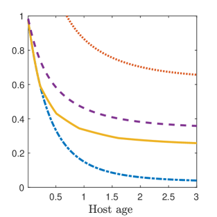
Figure 3 shows the four indices (Gini, Hoover, , and coefficient of variation) for a host in the Tallis-Leyton model with , , and . All four indices are strictly decreasing in host age. As in Figure 1, the Hoover index coincides with for and displays some discontinuity in the first derivative at points where the expectation is integer valued.
3.5. Parasite lifetime distribution
Our final comparison result concerns the parasite lifetime distribution. The result shows that variability in the parasite lifetimes decreases the variability in the host’s parasite burden. In particular, the result implies that the host’s parasite burden is most aggregated when parasites have constant lifetimes.
Theorem 8.
Suppose and has a single sign change with sign sequence so . Assume all other model parameters are equal, then .
Proof.
Assume For any set such that
As , it follows that . Let . Let have distribution (6) and let have the distribution (6) with replaced by and replaced by . The survival functions of and are
and
Since has a single sign change with sign sequence is , it follows that also has a single sign change with sign sequence . Applying Lemma 7 and Shaked and Shanthikumar (2007, Theorem 3.A.21) together shows . From Theorem 1, and , where and . Let be a sequence of independent random variables that are also independent of By construction . From the thinning property of the Poisson process, . As the convex order is closed under random sums, we see . Letting and noting that the convex order is closed under weak limits, we see . ∎
3.6. Asymptotic normality
As noted previously, for the host’s parasite burden to converge to a normal distribution, the coefficient of variation must tend to 0. In the Tallis-Leyton model, this is only possible when the rate of infective contacts tends to infinity.
Theorem 9.
Suppose there exists positive constants and such that
for all such that . Then
Proof.
The characteristic function of is . We aim to show that
| (7) |
The result then follows by Lévy’s convergence theorem. Define
For non-negative integers and real define
Then and
| (8) |
(Williams, 1991, pg 183). Note that
From the expressions for and ,
From the expression for and the fact that
we obtain
Using the bound (8) and the fact that , we see
and
Finally, using together with the bound (8) and the fact that , we see
Hence, the limit (7) holds. ∎
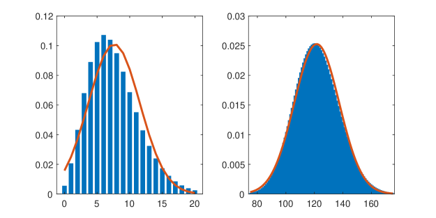
Figure 4 compares the probability mass function from the Tallis-Leyton model with the probability density function of the approximating normal distribution. The host was aged 3 with and . When , the probability mass function still shows some right skewness. The normal approximation in this instance places a non-negligible probability on values less than zero. When , the probability mass function is very close to symmetric and the normal distribution provides a good approximation. Figure 5 shows the Hoover and Gini indices together with the approximations based on asymptotic normality (4) and (5). In this instance the approximations appear reasonably accurate even for as small as 2, where the normal approximation fails.
4. Discussion
In this paper, we examined the aggregation of a host’s parasite burden in the Tallis-Leyton model, interpreting aggregation in terms of the Lorenz order. Our analysis showed that increasing the host’s age or the rate of infective contacts decreases aggregation. Similarly, increasing the aggregation of the clumps of parasites that enter the host as infective contacts also increases the aggregation of the host’s parasite burden. On the other hand, less variability in the parasite’s lifetime distribution, as defined in the convex order, results in greater aggregation of the host’s parasite burden.
Unfortunately, the population dynamics of parasites are often more complicated than what is represented in the Tallis-Leyton model. Some parasites need multiple hosts to complete its life cycle. Once a parasite finds a host it may be subject to intraspecific and interspecific competition for resources. Furthermore, parasites often interact with the host either by stimulating an immune response from the host or by increasing the host’s mortality rate.
Isham (1995) proposed a simple stochastic model that incorporate parasite induced host mortality. In Isham’s model, the host acquires parasites following the same dynamics as the Tallis-Leyton model and parasite lifetimes are assumed exponentially distributed. The important difference in Isham’s model is that each parasite present in the host increases the host’s death rate by a fixed amount . A complete analysis of Isham’s model in terms of the Lorenz order is beyond the scope of this paper. In a special case, however, we can see that parasite induced host mortality increases aggregation of the parasite distribution, as interpreted in the Lorenz order. When the number of parasites that enter the host at an infective contact follows a geometric distribution, an explicit expression for the limiting distribution is possible. Specifically, if , then
As the negative binomial distribution is decreasing in Lorenz order in both mean and , it follows that indices respecting the Lorenz order are increasing in the parasite induced host mortality rate. In contrast, the variance-to-mean ratio is so it is not affected by the parasite induced mortality.
A complete examination Isham’s model in terms of the Lorenz order may prove challenging. Even computing the Gini and Hoover indices may present difficulties since they require absolute moments, which are often not easily evaluated. In that case, the coefficient of variation may prove useful since it respects the Lorenz order, is easily evaluated, and can be used to approximate the Gini and Hoover indices when the distribution is approximately normal.
Data availability: Data sharing not applicable to this article as no datasets were generated or analysed during the current study.
References
- Abate and Whitt (1992) J. Abate and W. Whitt. Numerical inversion of probability generating functions. Oper. Res. Lett., 12:245–251, 1992.
- Adell and Cal (1994) J.A. Adell and J. De La Cal. Approximating gamma distributions by normalized negative binomial distributions. J. Appl. Probab., 31:391–400, 1994.
- Anderson and May (1978a) R.M. Anderson and R.M. May. Regulation and stability of host-parasite population interactions: I. regulatory processes. J. Anim. Ecol., 47:219–247, 1978a.
- Anderson and May (1978b) R.M. Anderson and R.M. May. Regulation and stability of host-parasite population interactions: II. destabilizing processes. J. Anim. Ecol., 47:249–267, 1978b.
- Arnold and Sarabia (2018) B.C. Arnold and J.M. Sarabia. Majorization and the Lorenz order with applications in applied mathematics and economics. Springer, New York, 2018.
- Barbour and Pugliese (2000) A.D. Barbour and A. Pugliese. On the variance-to-mean ratio in models of parasite distributions. Adv. Appl. Probab., 32:701–719, 2000.
- Gastwirth (1971) J.L. Gastwirth. A general definition of the Lorenz curve. Econometrica, 39:1037–1039, 1971.
- Gini (1924) C. Gini. Measurement of inequality of incomes. Econ. J., 31:124–126, 1924.
- Herbert and Isham (2000) J. Herbert and V. Isham. Stochastic host-parasite interaction models. J. Math. Biol., 40:343–371, 2000.
- Holman et al. (1983) D.F. Holman, M.L. Chaudhry, and B.R.K. Kashyap. On the service system . Eur. J. Oper. Res., 13:142–145, 1983.
- Isham (1995) V. Isham. Stochastic models of host-macroparasite interaction. Ann. Appl. Probab., 5:720–740, 1995.
- Lorenz (1905) M.O. Lorenz. Methods of measuring the concentration of wealth. Publication of the American Statistical Association, 9:209–219, 1905.
- McPherson et al. (2012) N.J. McPherson, R.A Norman, A.S. Hoyle, J.E. Bron, and N.G.H. Taylor. Stocking methods and parasite-induced reductions in capture: Modelling Argulus foliaceus in trout fisheries. J. Theor. Biol., 312:22–33, 2012.
- McVinish and Lester (2020) R. McVinish and R.J.G. Lester. Measuring aggregation in parasite populations. J. R. Soc. Interface, 17:20190886, 2020.
- McVinish and Lester (2024) R. McVinish and R.J.G. Lester. A graphical exploration of the relationship between parasite aggregation indices. arXiv:2409.03186, 2024.
- Morrill et al. (2023) A. Morrill, R. Poulin, and M.R. Forbes. Interrelationships and properties of parasite aggregation measures: a user’s guide. Int. J. Parasitol., 53:763–776, 2023.
- Peacock et al. (2018) S.J. Peacock, J. Bouhours, M.A. Lewis, and P.K. Molnár. Macroparasite dynamics of migratory host populations. Theor. Popul. Biol., 120:29–41, 2018.
- Pielou (1977) E.C. Pielou. Mathematical ecology. Wiley, New York, 1977.
- Poulin (1993) R. Poulin. The disparity between observed and uniform distributions: a new look at parasite aggregation. Int. J. Parasitol., 23:931–944, 1993.
- Poulin (2007) R. Poulin. Are there general laws in parasite ecology? Parasitol., 134:763–776, 2007.
- Rosa and Pugliese (2002) R. Rosa and A. Pugliese. Aggregation, stability, and oscillations in different models for host-macroparasite interactions. Theor. Popul. Biol., 61(3):319–334, 2002.
- Schreiber (2006) S.J. Schreiber. Host-parasitoid dynamics of a generalized thompson model. J. Math. Biol., 52:719–732, 2006.
- Schweder (1982) T. Schweder. On the dispersion of mixtures. Scand. J. Stat., 9:165–169, 1982.
- Shaked and Shanthikumar (2007) M. Shaked and J. G. Shanthikumar. Stochastic orders. Springer, New York, 2007.
- Shaw and Dobson (1995) D.J. Shaw and A.P. Dobson. Patterns of macroparasite abundance and aggregation in wildlife populations: a quantitative review. Parasitol., 111:S111–S133, 1995.
- Taguchi (1968) T. Taguchi. Concentration-curve methods and structures of skew populations. Ann. Inst. Stat. Math., 20:107–141, 1968.
- Tallis and Leyton (1969) G.M. Tallis and M.K. Leyton. Stochastic models of populations of helminthic parasites in the definitive host. I. Math. Biosci., 4:39–48, 1969.
- The MathWorks Inc. (2022a) The MathWorks Inc. Matlab version: 9.13.0.2080170 (r2022b) update 1, 2022a.
- The MathWorks Inc. (2022b) The MathWorks Inc. Symbolic math toolbox (r2022b), 2022b.
- Williams (1991) D. Williams. Probability with Martingales. Cambridge, 1991.
- Wilson et al. (2001) K. Wilson, O. Bjørnstad, A. Dobson, S. Merler, G. Poglayen, S. Randolph, A. Read, and A. Skorping. Heterogeneities in macroparasite infections: Patterns and processes. In P. Hudson, A. Rizzoli, B. Grenfell, H. Heesterbeek, and A. Dobson, editors, The Ecology of Wildlife Diseases, pages 6–44. Oxford University Press, 2001.