Randomized Subspace Derivative-Free Optimization with Quadratic Models and Second-Order Convergence

\nameCoralia Cartis^a and Lindon Roberts^b CONTACT L. Roberts. Email: [email protected] ^aMathematical Institute, University of Oxford, Radcliffe Observatory Quarter, Woodstock Road, Oxford OX2 6GG, UK; ^bSchool of Mathematics and Statistics, University of Sydney, Carslaw Building, Camperdown NSW 2006, Australia

Abstract

We consider model-based derivative-free optimization (DFO) for large-scale problems, based on iterative minimization in random subspaces. We provide the first worst-case complexity bound for such methods for convergence to approximate second-order critical points, and show that these bounds have significantly improved dimension dependence compared to standard full-space methods, provided low accuracy solutions are desired and/or the problem has low effective rank. We also introduce a practical subspace model-based method suitable for general objective minimization, based on iterative quadratic interpolation in subspaces, and show that it can solve significantly larger problems than state-of-the-art full-space methods, while also having comparable performance on medium-scale problems when allowed to use full-dimension subspaces.

keywords:

Derivative-free optimization; Large-scale optimization; Worst case complexity

^†^†articletype:

1 Introduction

In this work, we consider the problem of smooth nonlinear optimization where derivatives of the objective are unavailable, so-called derivative-free optimization (DFO) [13, 2, 24]. DFO methods are widely used across many fields [1], but in this work we focus on large-scale derivative-free problems, such as those arising from bilevel learning of variational models in imaging [17], fine-tuning large language models [25], adversarial example generation for neural networks [32], and as a possible proxy for global optimization methods in the high-dimensional setting [10]. Here we focus on the widely used class of model-based DFO methods, which are based on iteratively constructing local (interpolating) models for the objective.

Standard model-based methods [13, 24] suffer from a lack of scalability with respect to the problem dimension, coming from dimension-dependent interpolation error bounds affecting worst-case complexity, and significant per-iteration linear algebra costs; thus, they have traditionally been limited to small- or medium-scale problems. More recently, starting with [9], model-based DFO methods based on iterative minimization in random subspaces has proven to be a promising approach for tackling large-scale DFO problems in theory and practice. Theoretically, for example, using linear models in random subspaces improves the worst-case complexity of such methods from $O(n^{3}\epsilon^{-2})$ to $O(n^{2}\epsilon^{-2})$ evaluations to find an $\epsilon$ -approximate stationary point, for a problem with $n$ decision variables. This aligns with similar results for derivative-based optimization [5, 31] and other DFO approaches, such as direct search methods with random models [21, 30] and for gradient sampling in randomly drawn subspaces [23]. This model-based framework has been extended to handle stochastic objective values [16] and specialized to exploit structured quadratic model construction approaches [12]. The case of direct search methods in random subspaces has also been extended to the stochastic and nonsmooth case, and to show convergence to second-order optimal points [15].

There are alternative approaches for large-scale DFO where iterations are performed in subspaces that are deterministically generated from information from previous iterations, such as [36, 22, 33], where the method from [36, Chapter 5.3] alternates between iterations in two-dimensional subspaces and full-dimensional finite differencing. The method from [35] uses partially random subspaces, similar to [12], but is specialized to two-dimensional subspaces. We also note [26], where a full-dimensional model is updated at each iteration only inside a randomly generated subspace.

1.1 Contributions

Existing random subspace methods for model-based DFO have theoretical convergence to approximate first-order optimal points, but there is currently no theory handling second-order optimality in random subspace model-based DFO (with only [15] handling the direct search case). Although [12] does provide a mechanism for constructing fully quadratic interpolation models in random subspaces, which is a necessary component of second-order convergence theory, only first-order convergence theory is given. We also note the related work [3], which proves convergence to second-order optimal points for a trust-region method with probabilistic models and function values, which uses similar ideas but with different sources of uncertainty (instead of the approach here which uses randomly drawn subspaces with deterministic models and function values).

There are two main contributions in this work:

•

First, we show how the random subspace model-based method in [9] can be extended to allow convergence to second-order stationary points (similar to full space methods [13, 19]), and prove a high probability worst-case complexity bound for this method. Our approach is based on adapting a recent approach for second-order convergence of (derivative-based) subspace adaptive regularization with cubics [31, 11]. We show a worst-case complexity bound¹¹1The notation $\tilde{O}(\cdot)$ is the same as $O(\cdot)$ but hiding logarithmic factors as well as constants. of $\tilde{O}(n^{4.5}\epsilon^{-3})$ iterations and evaluations to achieve second-order optimality level $\epsilon$ for an $n$ -dimensional problem, a significant improvement on the $O(n^{9}\epsilon^{-3})$ iterations and $O(n^{11}\epsilon^{-3})$ evaluations for full space methods. For this theory to hold, we need to consider either low accuracy solutions or problems with low effective rank (i.e. low rank Hessians, such as fine-tuning large language models [25]). We note that the numerical evidence from [9] suggests that subspace methods are indeed most practical for finding low accuracy solutions.
•

We present a new practical algorithm for random subspace model-based DFO based on quadratic interpolation models. In [9], a practical approach based on linear interpolation models was built for nonlinear least-squares problems (a special case where linear models provide good practical performance [8]). Here, we extend this approach to handle general quadratic interpolation approaches, focusing in particular on underdetermined quadratic interpolation [28] in subspaces. Compared to state-of-the-art full-space methods using similar model constructions [4], our approach has comparable performance when set to use full-dimensional subspaces, but when using low-dimensional subspaces is able to solve larger problems (of dimension $n\approx O(1000)$ ) where existing approaches fail due to the significant linear algebra costs at this scale.

Structure

Firstly, in Section 2 we recall the random subspace model-based approach from [9] and its associated first-order complexity results. In Section 3 we extend this approach to find second-order critical points, stating the theoretical algorithm and proving the associated worst-case complexity bounds. Then, in Section 4 we outline our practical subspace method based on quadratic model construction in subspaces, which we test numerically in Section 5.

Notation

We use $\|\cdot\|$ to denote the Euclidean norm of vectors in and operator 2-norm of matrices, and $B(\bm{x},\Delta)=\{\bm{y}:\|\bm{y}-\bm{x}\|\leq\Delta\}$ is the closed ball of radius $\Delta$ centered at $\bm{x}$ . We use $\tilde{O}(\cdot)$ to denote $O(\cdot)$ with both logarithmic and constant factors omitted.

2 Background

In this work we consider the problem

\displaystyle\min_{\bm{x}\in\mathbb{R}^{n}}f(\bm{x}),

(1)

where $f:\mathbb{R}^{n}\to\mathbb{R}$ is continuously differentiable and nonconvex, but $\nabla f$ is not available. In standard model-based DFO, at iteration $k$ , we construct a local quadratic approximation for $f$ that we hope to be accurate near the current iterate $\bm{x}_{k}$ :

\displaystyle f(\bm{x}_{k}+\bm{s})\approx m_{k}(\bm{s}):=f(\bm{x}_{k})+\bm{g}_{k}^{T}\bm{s}+\frac{1}{2}\bm{s}^{T}H_{k}\bm{s},

(2)

for some $\bm{g}_{k}\in\mathbb{R}^{n}$ and (symmetric) $H_{k}\in\mathbb{R}^{n\times n}$ . This is typically achieved by finding $\bm{g}_{k}$ and $H_{k}$ to interpolate the value of $f$ at a collection of points near $\bm{x}_{k}$ . We then use this model inside a trust-region framework to ensure a globally convergent algorithm, where—compared to derivative-based trust-region methods—special care has to be taken to ensure that $m_{k}$ is sufficiently accurate and $\|\bm{g}_{k}\|$ is not too small relative to $\Delta_{k}$ , see e.g. [13] for details.

In the large-scale case, which would typically be $n\geq 1000$ for DFO, the linear algebra cost of model construction and management becomes significant, and the model error (relative to the true objective value) can grow rapidly. To avoid this issue, in [9] it was proposed to perform each iteration within a randomly drawn, low-dimensional subspace. Specifically, for some $p\ll n$ , at each iteration $k$ we generate a random $P_{k}\in\mathbb{R}^{n\times p}$ , defining an affine space $\mathcal{Y}_{k}:=\{\bm{x}_{k}+P_{k}\hat{\bm{s}}:\hat{\bm{s}}\in\mathbb{R}^{p}\}$ . We then construct a low-dimensional model to approximate $f$ only on $\mathcal{Y}_{k}$ ,

\displaystyle f(\bm{x}_{k}+P_{k}\hat{\bm{s}})\approx\hat{m}_{k}(\hat{\bm{s}}):=f(\bm{x}_{k})+\hat{\bm{g}}_{k}^{T}\bm{s}+\frac{1}{2}\hat{\bm{s}}^{T}\hat{H}_{k}\hat{\bm{s}},

(3)

for some $\hat{\bm{g}}_{k}\in\mathbb{R}^{p}$ and (symmetric) $\hat{H}_{k}\in\mathbb{R}^{p\times p}$ . We will adopt the convention where variables with hats are in the low-dimensional space and those without hats are in the full space. The trust-region framework is easily adapted to this situation: the model $\hat{m}_{k}$ is minimized subject to a ball constraint to get a tentative low-dimensional step $\hat{\bm{s}}_{k}$ , which in turn defines a new potential iterate $\bm{x}_{k}+P_{k}\hat{\bm{s}}_{k}$ , which may be accepted or rejected via a sufficient decrease test.

To achieve first-order convergence, the model $\hat{m}_{k}$ (3) must be sufficiently accurate in the following sense, [9, Definition 1].

Definition 2.1.

Given $\bm{x}\in\mathbb{R}^{n}$ , $\Delta>0$ and $P\in\mathbb{R}^{n\times p}$ , a model $\hat{m}:\mathbb{R}^{p}\to\mathbb{R}$ is $P$ -fully linear in $B(\bm{x},\Delta)$ if


$\displaystyle\|f(\bm{x}+P\hat{\bm{s}})-\hat{m}(\hat{\bm{s}})\|$	$\displaystyle\leq\kappa_{\textnormal{ef}}\Delta^{2},$	(4a)
$\displaystyle\\|P^{T}\nabla f(\bm{x}+P\hat{\bm{s}})-\nabla\hat{m}(\hat{\bm{s}})\\|$	$\displaystyle\leq\kappa_{\textnormal{eg}}\Delta,$	(4b)

for all $\hat{\bm{s}}\in\mathbb{R}^{p}$ with $\|\hat{\bm{s}}\|\leq\Delta$ , where the constants $\kappa_{\textnormal{ef}},\kappa_{\textnormal{eg}}>0$ are independent of $\bm{x}$ , $\Delta$ , $P$ and $\hat{m}$ .

1:Inputs: initial iterate

\bm{x}_{0}\in\mathbb{R}^{n}

, trust-region radii

0<\Delta_{0}\leq\Delta_{\max}

, trust-region updating parameters

0<\gamma_{\textnormal{dec}}<1<\gamma_{\textnormal{inc}}

, subspace dimension

p\in\{1,\ldots,n\}

, and success check parameters

\eta\in(0,1)

and

\mu>0

2:for

k=0,1,2,\ldots

3: Generate a random matrix

P_{k}\in\mathbb{R}^{n\times p}

satisfying Assumption 2.5.

4: Build a model

\hat{m}_{k}

(3) which is

P_{k}

-fully linear in

B(\bm{x}_{k},\Delta_{k})

5: Calculate a step by approximately solving the trust-region subproblem

\displaystyle\hat{\bm{s}}_{k}\approx\operatorname*{arg\,min}_{\hat{\bm{s}}\in\mathbb{R}^{p}}\hat{m}_{k}(\hat{\bm{s}}),\quad\text{s.t.}\>\>\|\hat{\bm{s}}\|\leq\Delta_{k}.

(5)

6: Evaluate

f(\bm{x}_{k}+P_{k}\hat{\bm{s}}_{k})

and calculate the ratio

\displaystyle R_{k}:=\frac{f(\bm{x}_{k})-f(\bm{x}_{k}+P_{k}\hat{\bm{s}}_{k})}{\hat{m}_{k}(\bm{0})-\hat{m}_{k}(\hat{\bm{s}}_{k})}.

(6)

7: if

R_{k}\geq\eta

and

\|\hat{\bm{g}}_{k}\|\geq\mu\Delta_{k}

then

8: (successful) Set

\bm{x}_{k+1}=\bm{x}_{k}+P_{k}\hat{\bm{s}}_{k}

and

\Delta_{k+1}=\min(\gamma_{\textnormal{inc}}\Delta_{k},\Delta_{\max})

9: else

10: (unsuccessful) Set

\bm{x}_{k+1}=\bm{x}_{k}

and

\Delta_{k+1}=\gamma_{\textnormal{dec}}\Delta_{k}

11: end if

12:end for

Algorithm 1 Random subspace DFO algorithm applied to (1), a simplified version of [9, Algorithm 1] based on [16, Algorithm 2.1].

A prototypical random subspace algorithm is presented in Algorithm 1. It is a simplification of the original algorithm [9, Algorithm 1], which includes a more sophisticated trust-region management procedure based on [29] and allows the model $\hat{m}_{k}$ to not be $P_{k}$ -fully linear at all iterations. The version presented here is based on [16, Algorithm 2.1] and has the same first-order convergence guarantees.

In order to prove convergence of Algorithm 1, we need the following standard assumptions on the objective function, model and trust-region subproblem calculation (5).

Assumption 2.2.

The objective function $f:\mathbb{R}^{n}\to\mathbb{R}$ in (1) is bounded below by $f_{\textnormal{low}}$ and is continuously differentiable, where $\nabla f$ is $L_{\nabla f}$ -Lipschitz continuous for some $L_{\nabla f}>0$ .

Assumption 2.3.

The model Hessians $\hat{H}_{k}$ are uniformly bounded, $\|\hat{H}_{k}\|\leq\kappa_{H}$ for all $k$ , for some $\kappa_{H}\geq 1$ .

Assumption 2.4.

The computed solution $\hat{\bm{s}}_{k}$ in (5) satisfies the Cauchy decrease condition

\displaystyle\hat{m}_{k}(\bm{0})-\hat{m}_{k}(\hat{\bm{s}}_{k})\geq c_{1}\|\hat{\bm{g}}_{k}\|\min\left(\Delta_{k},\frac{\|\hat{\bm{g}}_{k}\|}{\max(\|\hat{H}_{k}\|,1)}\right),

(7)

for some $c_{1}\in[1/2,1]$ independent of $k$ .

While the above assumptions are common for trust-region methods, we need an additional assumption on the random matrices $P_{k}$ defining the subspace at each iteration.

Assumption 2.5.

The matrices $P_{k}$ are uniformly bounded, $\|P_{k}\|\leq P_{\max}$ for all $k$ , and at each iteration $P_{k}$ is well-aligned, i.e.

\displaystyle\mathbb{P}\left[\|P_{k}^{T}\nabla f(\bm{x}_{k})\|\geq\alpha\|\nabla f(\bm{x}_{k})\|\right]\geq 1-\delta,

(8)

for some $\alpha>0$ and $\delta\in(0,1)$ independent of $k$ and all previous iterations $P_{0},\ldots,P_{k-1}$ .

Although condition (8) depends on $\nabla f(\bm{x}_{k})$ , which is not available, Assumption 2.5 can still be satisfied using Johnson-Lindenstrauss transforms [34]. For example, $P_{k}$ may have independent $N(0,1/p)$ entries or be the first $p$ columns of a random orthogonal $n\times n$ matrix scaled by $\sqrt{n/p}$ . More details on how Assumption 2.5 may be satisfied can be found in [31, Chapter 4], [5, Section 3.2], [9, Section 2.6], [16, Section 3.1], [30, Section 3.3], or [12, Section 2.5], for example. Most crucially, for such constructions, (8) can be satisfied for $p=\mathcal{O}(1)$ independent of $n$ .

Under these assumptions, Algorithm 1 has a first-order worst-case complexity bound of the following form (e.g. [9, Corollary 1] or [12, Theorem 9]).

Theorem 2.6.

Suppose Assumptions 2.2, 2.3, 2.4 and 2.5 hold. Suppose also that $\gamma_{\textnormal{inc}}>\gamma_{\textnormal{dec}}^{-2}$ and $\delta$ sufficiently small in Assumption 2.5. Then for $k$ sufficiently large, the iterates of Algorithm 1 satisfy

\displaystyle\mathbb{P}\left[\min_{j\leq k}\|\nabla f(\bm{x}_{j})\|\leq\frac{C\sqrt{\kappa_{H}}\,\kappa_{d}}{\sqrt{k}}\right]\geq 1-e^{-ck},

(9)

for constants $c,C>0$ , where $\kappa_{d}:=\max(\kappa_{\textnormal{ef}},\kappa_{\textnormal{eg}})$ from Definition 2.1.

This result implies that $\|\nabla f(\bm{x}_{k})\|$ is driven below $\epsilon$ for the first time after $\mathcal{O}(\kappa_{H}\kappa_{d}^{2}\epsilon^{-2})$ iterations and $\mathcal{O}(p\kappa_{H}\kappa_{d}^{2}\epsilon^{-2})$ objective evaluations (with high probability), assuming $\mathcal{O}(p)$ interpolation points are used to construct $\hat{m}_{k}$ . Assuming linear interpolation models, we have $\kappa_{d}=\mathcal{O}(P_{\max}^{2}p)$ and $\kappa_{H}=1$ , so in the full-space case $p=n$ and $P_{k}=I_{n\times n}$ we get a worst-case complexity of $\mathcal{O}(n^{2}\epsilon^{-2})$ iterations and $\mathcal{O}(n^{3}\epsilon^{-2})$ objective evaluations. However, using a Johnson-Lindenstrauss transform we may use $p=\mathcal{O}(1)$ and $P_{\max}=\mathcal{O}(\sqrt{n})$ , giving the same iteration complexity but an improved complexity of $\mathcal{O}(n^{2}\epsilon^{-2})$ evaluations.

3 Convergence to Second-Order Stationary Points

We now consider the extension of the framework in Section 2 to a second-order convergent algorithm. Our basic framework is the same, namely at each iteration we select a random $P_{k}$ and build a low-dimensional model $\hat{m}_{k}$ (3) to approximate $f$ in the corresponding affine space $\mathcal{Y}_{k}$ .

Now, we are interested in the second-order criticality measure

\displaystyle\sigma_{k}:=\max(\|\nabla f(\bm{x}_{k})\|,\tau_{k}),\qquad\text{where}\qquad\tau_{k}:=\max(-\lambda_{\min}(\nabla^{2}f(\bm{x}_{k})),0)),

(10)

(see [13, Chapter 10], for example). Restricting the objective to the space $\mathcal{Y}_{k}$ we get the corresponding subspace criticality measure

\displaystyle\hat{\sigma}_{k}:=\max(\|P_{k}^{T}\nabla f(\bm{x}_{k})\|,\hat{\tau}_{k}),\qquad\text{where}\qquad\hat{\tau}_{k}:=\max(-\lambda_{\min}(P_{k}^{T}\nabla^{2}f(\bm{x}_{k})P_{k}),0)),

(11)

and our interpolation model $\hat{m}_{k}$ defines its own approximate (subspace) criticality measure

\displaystyle\hat{\sigma}^{m}_{k}:=\max(\|\hat{\bm{g}}_{k}\|,\hat{\tau}^{m}_{k}),\qquad\text{where}\qquad\hat{\tau}^{m}_{k}:=\max(-\lambda_{\min}(\hat{H}_{k}),0)).

(12)

To achieve $\sigma_{k}\to 0$ (i.e. convergence to second-order critical points), we need a more restrictive notion of model accuracy.

Definition 3.1.

The subspace model $\hat{m}_{k}:\mathbb{R}^{p}\to\mathbb{R}$ in (3) is $P_{k}$ -fully quadratic if there exist constants $\kappa_{\textnormal{ef}},\kappa_{\textnormal{eg}},\kappa_{\textnormal{eh}}$ independent of $k$ such that


$\displaystyle\|f(\bm{x}_{k}+P_{k}\hat{\bm{s}})-\hat{m}_{k}(\hat{\bm{s}})\|$	$\displaystyle\leq\kappa_{\textnormal{ef}}\Delta_{k}^{3},$	(13a)
$\displaystyle\\|P_{k}^{T}\nabla f(\bm{x}_{k}+P_{k}\hat{\bm{s}})-\nabla\hat{m}_{k}(\hat{\bm{s}})\\|$	$\displaystyle\leq\kappa_{\textnormal{eg}}\Delta_{k}^{2},$	(13b)
$\displaystyle\\|P_{k}^{T}\nabla^{2}f(\bm{x}_{k}+P_{k}\hat{\bm{s}})P_{k}-\nabla^{2}\hat{m}_{k}(\hat{\bm{s}})\\|$	$\displaystyle\leq\kappa_{\textnormal{eh}}\Delta_{k},$	(13c)

for all $\|\hat{\bm{s}}\|\leq\Delta_{k}$ .

This notion is discussed in [12, Section 2.4], and a specific sampling mechanism for achieving this is described there.

1:Inputs: initial iterate

\bm{x}_{0}\in\mathbb{R}^{n}

and trust-region radius

\Delta_{0}>0

, and subspace dimension

p\in\{1,\ldots,n\}

2:Parameters: maximum trust-region radius

\Delta_{\max}\geq\Delta_{0}

, trust-region parameters

0<\gamma_{\textnormal{dec}}<1<\gamma_{\textnormal{inc}}

, and step acceptance thresholds

\eta\in(0,1)

and

\mu>0

3:for

k=0,1,2,\ldots

4: Select a random matrix

P_{k}\in\mathbb{R}^{n\times p}

satisfying Assumption 3.7

5: Build subspace model

\hat{m}_{k}

(3) which is

P_{k}

-fully quadratic (Definition 3.1).

6: Calculate a step

\hat{\bm{s}}_{k}

by approximately solving the trust-region subproblem (5).

7: Evaluate

f(\bm{x}_{k}+P_{k}\hat{\bm{s}}_{k})

and calculate the ratio

R_{k}

(6).

8: if

R_{k}\geq\eta

and

\hat{\sigma}^{m}_{k}\geq\mu\Delta_{k}

then

9: (successful) Set

\bm{x}_{k+1}=\bm{x}_{k}+P_{k}\hat{\bm{s}}_{k}

and

\Delta_{k+1}=\min(\gamma_{\textnormal{inc}}\Delta_{k},\Delta_{\max})

10: else

11: (unsuccessful) Set

\bm{x}_{k+1}=\bm{x}_{k}

and

\Delta_{k+1}=\gamma_{\textnormal{dec}}\Delta_{k}

12: end if

13:end for

Algorithm 2 Random-subspace model-based DFO algorithm applied to (1) with second-order convergence.

In addition, we need the following assumptions on the objective and computed trust-region step which are standard for second-order convergence (e.g. [13, Chapter 10]).

Assumption 3.2.

The objective $f$ is bounded below by $f_{\textnormal{low}}$ , and is twice continuously differentiable and $\nabla^{2}f$ is $L_{H}$ -Lipschitz continuous. Additionally, the Hessian at all iterates is uniformly bounded, $\|\nabla^{2}f(\bm{x}_{k})\|\leq M$ for some $M>0$ independent of $k$ .

Assumption 3.3.

The step $\hat{\bm{s}}_{k}$ satisfies

\displaystyle\hat{m}_{k}(\bm{0})-\hat{m}_{k}(\hat{\bm{s}}_{k})\geq\kappa_{s}\max\left(\|\hat{\bm{g}}_{k}\|\min\left(\Delta_{k},\frac{\|\hat{\bm{g}}_{k}\|}{\max(\|\hat{H}_{k}\|,1)}\right),\hat{\tau}^{m}_{k}\Delta_{k}^{2}\right),

(14)

for some $\kappa_{s}>0$ independent of $k$ .

We also require Assumption 2.3 (bounded model Hessians) holds here.

Lemma 3.4 (Lemma 10.15, [13]).

Suppose Assumption 3.2 holds and $\hat{m}_{k}$ is $P_{k}$ -fully quadratic on $B(\bm{x}_{k},\Delta_{k})$ . Then $|\hat{\sigma}_{k}-\hat{\sigma}^{m}_{k}|\leq\kappa_{\sigma}\Delta_{k}$ , where $\kappa_{\sigma}:=\max(\kappa_{\textnormal{eg}}\Delta_{\max},\kappa_{\textnormal{eh}})$ .

Lemma 3.5.

Suppose Assumptions 2.3 and 3.3 hold. If

\displaystyle\Delta_{k}\leq c_{0}\,\hat{\sigma}^{m}_{k},\qquad\text{where}\qquad c_{0}:=\min\left(\frac{1}{\mu},\frac{1}{\kappa_{H}},\frac{\kappa_{s}(1-\eta)}{\kappa_{\textnormal{ef}}\Delta_{\max}},\frac{\kappa_{s}(1-\eta)}{\kappa_{\textnormal{ef}}}\right),

(15)

then iteration $k$ is successful (i.e. $R_{k}\geq\eta$ and $\hat{\sigma}^{m}_{k}\geq\mu\Delta_{k}$ ).

Proof.

This argument is based on [13, Lemma 10.17]. First, since $c_{0}\leq 1/\mu$ , we immediately have $\hat{\sigma}^{m}_{k}\geq\mu\Delta_{k}$ ; it remains to show $R_{k}\geq\eta$ . By definition of $\hat{\sigma}^{m}_{k}$ , we either have $\hat{\sigma}^{m}_{k}=\|\hat{\bm{g}}_{k}\|$ or $\hat{\sigma}^{m}_{k}=\hat{\tau}^{m}_{k}$ . From Assumptions 3.3 and 2.3, we have

\displaystyle\hat{m}_{k}(\bm{0})-\hat{m}_{k}(\hat{\bm{s}}_{k})\geq\kappa_{s}\max\left(\|\hat{\bm{g}}_{k}\|\min\left(\Delta_{k},\frac{\|\hat{\bm{g}}_{k}\|}{\kappa_{H}}\right),\hat{\tau}^{m}_{k}\Delta_{k}^{2}\right).

(16)

First, if $\hat{\sigma}^{m}_{k}=\|\hat{\bm{g}}_{k}\|$ , then $\Delta_{k}\leq\frac{1}{\kappa_{H}}\hat{\sigma}^{m}_{k}=\frac{1}{\kappa_{H}}\|\hat{\bm{g}}_{k}\|$ implies

\displaystyle\hat{m}_{k}(\bm{0})-\hat{m}_{k}(\hat{\bm{s}}_{k})\geq\kappa_{s}\|\hat{\bm{g}}_{k}\|\Delta_{k}=\kappa_{s}\hat{\sigma}^{m}_{k}\Delta_{k}.

(17)

Then we have

$\displaystyle\|R_{k}-1\|$	$\displaystyle=\frac{\|f(\bm{x}_{k}+P_{k}\hat{\bm{s}}_{k})-\hat{m}_{k}(\hat{\bm{s}}_{k})\|}{\|\hat{m}_{k}(\bm{0})-\hat{m}_{k}(\hat{\bm{s}}_{k})\|},$	(18)
	$\displaystyle\leq\frac{\kappa_{\textnormal{ef}}\Delta_{k}^{3}}{\kappa_{s}\hat{\sigma}^{m}_{k}\Delta_{k}},$	(19)
	$\displaystyle\leq\frac{\kappa_{\textnormal{ef}}\Delta_{\max}}{\kappa_{s}\hat{\sigma}^{m}_{k}}\Delta_{k},$	(20)

and so $|R_{k}-1|\leq 1-\eta$ (by definition of $c_{0}$ ), and hence $R_{k}\geq\eta$ as required. Alternatively, if $\hat{\sigma}^{m}_{k}=\hat{\tau}^{m}_{k}$ , then

\displaystyle\hat{m}_{k}(\bm{0})-\hat{m}_{k}(\hat{\bm{s}}_{k})\geq\kappa_{s}\hat{\tau}^{m}_{k}\Delta_{k}^{2}=\kappa_{s}\hat{\sigma}^{m}_{k}\Delta_{k}^{2}.

(21)

In this case, we get

\displaystyle|R_{k}-1|

\displaystyle=\frac{|f(\bm{x}_{k}+P_{k}\hat{\bm{s}}_{k})-\hat{m}_{k}(\hat{\bm{s}}_{k})|}{|\hat{m}_{k}(\bm{0})-\hat{m}_{k}(\hat{\bm{s}}_{k})|}\leq\frac{\kappa_{\textnormal{ef}}\Delta_{k}^{3}}{\kappa_{s}\hat{\sigma}^{m}_{k}\Delta_{k}^{2}}=\frac{\kappa_{\textnormal{ef}}\Delta_{k}}{\kappa_{s}\hat{\sigma}^{m}_{k}},

(22)

and so again $|R_{k}-1|\leq 1-\eta$ by definition of $c_{0}$ , and $R_{k}\geq\eta$ . ∎

Now, we need to specify our requirements for a well-aligned subspace. This is based on the approach in [11], originally from the PhD thesis [31, Chapter 5.6]. At iteration $k$ , suppose $\nabla^{2}f(\bm{x}_{k})$ has eigendecomposition $\nabla^{2}f(\bm{x}_{k})=\sum_{i=1}^{r}\lambda_{i}\bm{v}_{i}\bm{v}_{i}^{T}$ , where $\lambda_{1}\geq\lambda_{2}\geq\cdots\geq\lambda_{r}$ and $r:=\operatorname{rank}(\nabla^{2}f(\bm{x}_{k}))\leq n$ , and $\bm{v}_{1},\ldots,\bm{v}_{r}$ are orthonormal. Define $\hat{\bm{v}}_{i}:=P_{k}^{T}\bm{v}_{i}\in\mathbb{R}^{p}$ , and so the (true) subspace Hessian is $P_{k}^{T}\nabla^{2}f(\bm{x}_{k})P_{k}=\sum_{i=1}^{r}\lambda_{i}\hat{\bm{v}}_{i}\hat{\bm{v}}_{i}^{T}$ .

Definition 3.6.

A subspace $P_{k}$ is well-aligned if


$\displaystyle\\|P_{k}\\|$	$\displaystyle\leq P_{\max},$	(23a)
$\displaystyle\\|P_{k}^{T}\nabla f(\bm{x}_{k})\\|$	$\displaystyle\geq(1-\alpha)\\|\nabla f(\bm{x}_{k})\\|,$	(23b)
$\displaystyle\\|\hat{\bm{v}}_{r}\\|$	$\displaystyle\geq 1-\alpha,$	(23c)
$\displaystyle(\hat{\bm{v}}_{i}^{T}\hat{\bm{v}}_{r})^{2}$	$\displaystyle\leq 4\alpha^{2},\qquad\forall i=1,\ldots,r-1,$	(23d)

for some $\alpha\in(0,1)$ and $P_{\max}>0$ independent of $k$ .

In practice, a well-aligned subspace can be achieved by generating $P_{k}$ randomly (see Section 3.1 below). Hence, we use the following assumption.

Assumption 3.7.

At any iteration $k$ , the matrix $P_{k}$ is well-aligned in the sense of Definition 3.6 with probability at least $1-\delta_{S}$ , for some $\delta_{S}\in[0,1)$ , independent of all previous iterations $P_{0},\ldots,P_{k-1}$ .

The first two well-aligned properties (23a) and (23b) match the first-order case (Assumption 2.5); i.e. the subspace sees a sizeable fraction of the true gradient. The third condition (23c) says the subspace sees a sizeable fraction of the left-most eigenvector (since $\|\bm{v}_{r}\|=1$ ), and the last condition (23d) says the first $r-1$ eigenvectors remain approximately orthogonal to the last eigenvector in the subspace.

Lemma 3.8.

Suppose Assumption 3.2 holds. If $P_{k}$ is well-aligned and $\sigma_{k}\geq\epsilon>0$ , and

\displaystyle\theta:=(1-\alpha)^{2}-\frac{4M(r-1)\alpha^{2}}{\epsilon(1-\alpha)^{2}}>0.

(24)

Then

\displaystyle\hat{\sigma}_{k}\geq\min((1-\alpha)^{2},\theta)\epsilon.

(25)

Proof.

This argument is based on [11, Lemma 6.10], originally from [31, Lemma 5.6.6]. First, suppose that $\sigma_{k}=\|\nabla f(\bm{x}_{k})\|$ . Then

\displaystyle\hat{\sigma}_{k}\geq\|P_{k}^{T}\nabla f(\bm{x}_{k})\|\geq(1-\alpha)\|\nabla f(\bm{x}_{k})\|=(1-\alpha)\sigma_{k}\geq(1-\alpha)^{2}\epsilon,

(26)

using $(1-\alpha)^{2}<1-\alpha$ from $\alpha\in(0,1)$ and we are done. Instead, suppose that $\sigma_{k}=\tau_{k}$ . Using Rayleigh quotients, we have

\displaystyle\lambda_{\min}(P_{k}^{T}\nabla^{2}f(\bm{x}_{k})P_{k})\leq\frac{\hat{\bm{v}}_{r}^{T}(\sum_{i=1}^{r}\lambda_{i}\hat{\bm{v}}_{i}\hat{\bm{v}}_{i}^{T})\hat{\bm{v}}_{r}}{\|\hat{\bm{v}}_{r}\|^{2}}=\lambda_{r}\|\hat{\bm{v}}_{r}\|^{2}+\frac{\sum_{i=1}^{r-1}\lambda_{i}(\hat{\bm{v}}_{i}^{T}\hat{\bm{v}}_{r})^{2}}{\|\hat{\bm{v}}_{r}\|^{2}}.

(27)

Since $\tau_{k}\geq\epsilon>0$ , we have $\tau_{k}=-\lambda_{r}$ and $\lambda_{r}<-\epsilon$ , and so

\displaystyle-\lambda_{\min}(P_{k}^{T}\nabla^{2}f(\bm{x}_{k})P_{k})

\displaystyle\geq\epsilon\|\hat{\bm{v}}_{r}\|^{2}-\lambda_{1}\frac{\sum_{i=1}^{r-1}(\hat{\bm{v}}_{i}^{T}\hat{\bm{v}}_{r})^{2}}{\|\hat{\bm{v}}_{r}\|^{2}}.

(28)

If $\lambda_{1}\leq 0$ then the second term is non-negative, and so

\displaystyle-\lambda_{\min}(P_{k}^{T}\nabla^{2}f(\bm{x}_{k})P_{k})\geq\epsilon(1-\alpha)^{2}>0,

(29)

and so $\hat{\tau}_{k}>0$ with $\hat{\sigma}_{k}\geq\hat{\tau}_{k}\geq\epsilon(1-\alpha)^{2}$ . Instead, if $\lambda_{1}>0$ then $\lambda_{1}\leq\|\nabla^{2}f(\bm{x}_{k})\|\leq M$ and so we have

\displaystyle-\lambda_{\min}(P_{k}^{T}\nabla^{2}f(\bm{x}_{k})P_{k})

\displaystyle\geq\epsilon(1-\alpha)^{2}-M\frac{4(r-1)\alpha^{2}}{(1-\alpha)^{2}}=\theta\epsilon>0,

(30)

and so again $-\lambda_{\min}(P_{k}^{T}\nabla^{2}f(\bm{x}_{k})P_{k})<0$ yielding $\hat{\sigma}_{k}\geq\hat{\tau}_{k}>\theta\epsilon$ and the result follows. ∎

Lemma 3.9.

Suppose Assumption 3.2 holds and $\theta>0$ (24). If $P_{k}$ is well-aligned and $\sigma_{k}\geq\epsilon$ , then if iteration $k$ is successful,

\displaystyle\hat{\sigma}^{m}_{k}\geq c_{1}\epsilon,\qquad\text{where}\qquad c_{1}:=\frac{\min(1-\alpha,(1-\alpha)^{2},\theta)}{1+\kappa_{\sigma}\mu^{-1}}.

(31)

Proof.

On successful iterations, we have $\hat{\sigma}^{m}_{k}\geq\mu\Delta_{k}$ and so from Lemmas 3.4 and 3.8 we have

\displaystyle\min(1-\alpha,(1-\alpha)^{2},\theta)\epsilon\leq\hat{\sigma}_{k}\leq\hat{\sigma}^{m}_{k}+|\hat{\sigma}_{k}-\hat{\sigma}^{m}_{k}|\leq\hat{\sigma}^{m}_{k}+\kappa_{\sigma}\Delta_{k}\leq(1+\kappa_{\sigma}\mu^{-1})\hat{\sigma}^{m}_{k},

(32)

and we are done. ∎

We are now ready to prove the worst-case complexity of Algorithm 2 to (approximate) second-order stationary points. The below closely follows the argument from [9], used to prove Theorem 2.6. For a fixed $K$ , define the following sets of iterations:

•

$\mathcal{A}$ is the set of iterations in $\{0,\ldots,K\}$ for which $P_{k}$ is well-aligned.
•

$\mathcal{A}^{C}$ is the set of iterations in $\{0,\ldots,K\}$ for which $P_{k}$ is not well-aligned.
•

$\mathcal{S}$ (resp. $\mathcal{U}$ ) is the set of iterations in $\{0,\ldots,K\}$ which are successful (resp. unsuccessful).
•

$\mathcal{D}(\Delta)$ is the set of iterations in $\{0,\ldots,K\}$ for which $\Delta_{k}\geq\Delta$ .
•

$\mathcal{D}^{C}(\Delta)$ is the set of iterations in $\{0,\ldots,K\}$ for which $\Delta_{k}<\Delta$ .

Hence, for any $K$ and $\Delta$ , we have the partitions $\{0,\ldots,K\}=\mathcal{A}\cup\mathcal{A}^{C}=\mathcal{S}\cup\mathcal{U}=\mathcal{D}(\Delta)\cup\mathcal{D}^{C}(\Delta)$ , as well as $\mathcal{D}(\Delta_{1})\subseteq\mathcal{D}(\Delta_{2})$ if $\Delta_{1}\geq\Delta_{2}$ .

We first use standard trust-region arguments to bound $\mathcal{A}$ (by considering the four cases $\mathcal{A}\cap\mathcal{D}(\Delta)\cap\mathcal{S},\ldots,\mathcal{A}\cap\mathcal{D}^{C}(\Delta)\cap\mathcal{U}$ separately), provided $\sigma_{k}$ remains large. We can then bound (to high probability) the total number of iterations $K$ for which $\sigma_{k}$ is large by noting that $\mathcal{A}^{C}$ occurs with small probability (Assumption 3.7).

Lemma 3.10.

Suppose Assumptions 2.3, 3.2 and 3.3 hold, and $\theta>0$ (24). If $\sigma_{k}\geq\epsilon>0$ for all $k\leq K$ , then

\displaystyle\#(\mathcal{A}\cap\mathcal{D}(\Delta)\cap\mathcal{S})\leq\phi(\Delta,\epsilon),\qquad\text{where}\quad\phi(\Delta,\epsilon):=\frac{f(\bm{x}_{0})-f_{\textnormal{low}}}{\eta\kappa_{s}c_{1}\min(\epsilon\Delta,\epsilon\Delta^{2})},

(33)

where $c_{1}>0$ is defined in Lemma 3.9.

Proof.

From (17) and (21), we have

\displaystyle\hat{m}_{k}(\bm{0})-\hat{m}_{k}(\hat{\bm{s}}_{k})\geq\min(\kappa_{s}\hat{\sigma}^{m}_{k}\Delta_{k},\kappa_{s}\hat{\sigma}^{m}_{k}\Delta_{k}^{2}),

(34)

depending on whether $\hat{\sigma}^{m}_{k}=\|\hat{\bm{g}}_{k}\|$ or $\hat{\sigma}^{m}_{k}=\hat{\tau}^{m}_{k}$ . For $k\in\mathcal{A}\cap\mathcal{D}(\Delta)$ , from Lemma 3.9 we have $\Delta_{k}\geq\Delta$ and $\hat{\sigma}^{m}_{k}\geq c_{1}\epsilon$ and so

\displaystyle\hat{m}_{k}(\bm{0})-\hat{m}_{k}(\hat{\bm{s}}_{k})\geq\kappa_{s}c_{1}\min(\epsilon\Delta,\epsilon\Delta^{2}).

(35)

We note that $\bm{x}_{k}$ is only changed for $k\in\mathcal{S}$ , and so

\displaystyle f(\bm{x}_{0})-f_{\textnormal{low}}\geq\sum_{k\in\mathcal{S}}f(\bm{x}_{k})-f(\bm{x}_{k}+P_{k}\hat{\bm{s}}_{k})\geq\sum_{k\in\mathcal{A}\cap\mathcal{D}(\Delta)\cap\mathcal{S}}\eta(\hat{m}_{k}(\bm{0})-\hat{m}_{k}(\hat{\bm{s}}_{k})),

(36)

which yields

\displaystyle f(\bm{x}_{0})-f_{\textnormal{low}}\geq\eta\kappa_{s}c_{1}\min(\epsilon\Delta,\epsilon\Delta^{2})\cdot\#(\mathcal{A}\cap\mathcal{D}(\Delta)\cap\mathcal{S}),

(37)

which gives the result. ∎

Lemma 3.11.

Suppose Assumptions 2.3, 3.2 and 3.3 hold, and $\theta>0$ (24). If $\sigma_{k}\geq\epsilon>0$ for all $k\leq K$ , then

\displaystyle\#(\mathcal{A}\cap\mathcal{D}^{C}(\Delta)\cap\mathcal{U})=0,

(38)

for all $\Delta\leq c_{2}\epsilon$ , where

\displaystyle c_{2}:=\frac{1}{\kappa_{\sigma}+c_{0}^{-1}}\min(1-\alpha,(1-\alpha)^{2},\theta),

(39)

where $\kappa_{\sigma}>0$ is defined in Lemma 3.4 and $c_{0}>0$ is defined in Lemma 3.5.

Proof.

This argument follows [19, Lemma 4.2.3]. To find a contradiction, suppose $k\in\mathcal{A}\cap\mathcal{D}^{C}(\Delta)\cap\mathcal{U}$ . Since $k\in\mathcal{A}$ , we have $\hat{\sigma}_{k}\geq\min(1-\alpha,(1-\alpha)^{2},\theta)\epsilon$ by Lemma 3.8. Also, since $k\in\mathcal{U}$ , we must have $\Delta_{k}>c_{0}\hat{\sigma}^{m}_{k}$ by Lemma 3.5. Thus,

\displaystyle\min(1-\alpha,(1-\alpha)^{2},\theta)\epsilon\leq\hat{\sigma}_{k}\leq(\hat{\sigma}_{k}-\hat{\sigma}^{m}_{k})+\hat{\sigma}^{m}_{k}<\kappa_{\sigma}\Delta_{k}+c_{0}^{-1}\Delta_{k},

(40)

where the last inequality follows from Lemma 3.4. By assumption on $\Delta$ , this contradicts $k\in\mathcal{D}^{C}(\Delta)$ , and we are done. ∎

Lemma 3.12.

Suppose Assumptions 2.3, 3.2 and 3.3 hold, and $\theta>0$ (24). If $\sigma_{k}\geq\epsilon>0$ for all $k\leq K$ , then

\displaystyle\#(\mathcal{D}(\gamma_{\textnormal{dec}}^{-1}\Delta)\cap\mathcal{U})

\displaystyle\leq c_{3}\cdot\#(D(\gamma_{\textnormal{inc}}^{-1}\Delta)\cap\mathcal{S})+c_{4}(\Delta),

(41)

for all $\Delta\leq\Delta_{0}$ , and

\displaystyle\#(\mathcal{D}^{C}(\gamma_{\textnormal{inc}}^{-1}\Delta)\cap\mathcal{S})

\displaystyle\leq c_{3}^{-1}\cdot\#(\mathcal{D}^{C}(\gamma_{\textnormal{dec}}^{-1}\Delta)\cap\mathcal{U}),

(42)

for all $\Delta\leq\min(\Delta_{0},\gamma_{\textnormal{inc}}^{-1}\Delta_{\max})$ , where we define

\displaystyle c_{3}:=\frac{\log(\gamma_{\textnormal{inc}})}{\log(\gamma_{\textnormal{dec}}^{-1})},\qquad\text{and}\qquad c_{4}(\Delta):=\frac{\log(\Delta_{0}/\Delta)}{\log(\gamma_{\textnormal{dec}}^{-1})}.

(43)

Proof.

This follows the same argument as in [9, Lemmas 6 & 7], which we include here for completeness. In both cases, we consider the movement of $\log(\Delta_{k})$ , which is increased by at most $\log(\gamma_{\textnormal{inc}})$ if $k\in\mathcal{S}$ and decreased by $\log(\gamma_{\textnormal{dec}}^{-1})$ if $k\in\mathcal{U}$ .

To show (41), we note:

•

Since $\Delta\leq\Delta_{0}$ , the value $\log(\Delta)$ is $\log(\Delta_{0}/\Delta)$ below the starting value $\log(\Delta_{0})$ .
•

If $k\in\mathcal{S}$ , then $\log(\Delta_{k})$ increases by at most $\log(\gamma_{\textnormal{inc}})$ , and $\Delta_{k+1}\geq\Delta$ is only possible if $\Delta_{k}\geq\gamma_{\textnormal{inc}}^{-1}\Delta$ .
•

If $k\in\mathcal{U}$ , then $\log(\Delta_{k})$ is decreased by $\log(\gamma_{\textnormal{dec}}^{-1})$ and $\Delta_{k+1}\geq\Delta$ if $\Delta_{k}\geq\gamma_{\textnormal{dec}}^{-1}\Delta$ .

Hence the total decrease in $\log(\Delta_{k})$ from $k\in\mathcal{D}(\gamma_{\textnormal{dec}}^{-1})\cap\mathcal{U}$ must be fully matched by the initial gap $\log(\Delta_{0}/\Delta)$ plus the maximum possible amount that $\log(\Delta_{k})$ can be increased above $\log(\Delta)$ ; that is,

\displaystyle\log(\gamma_{\textnormal{dec}}^{-1})\#(\mathcal{D}(\gamma_{\textnormal{dec}}^{-1}\Delta)\cap\mathcal{S})\leq\log(\Delta_{0}/\Delta)+\log(\gamma_{\textnormal{inc}})\#(\mathcal{D}(\gamma_{\textnormal{inc}}^{-1}\Delta)\cap\mathcal{S}),

(44)

and we get (41).

To get (42), we use a similar approach. Specifically,

•

If $k\in\mathcal{S}$ , then since $\Delta\leq\gamma_{\textnormal{inc}}^{-1}\Delta_{\max}$ , we have $\log(\Delta_{k})$ is increased by exactly $\log(\gamma_{\textnormal{inc}})$ , and $\Delta_{k+1}<\Delta$ if and only if $\Delta_{k}<\gamma_{\textnormal{inc}}^{-1}\Delta$ .
•

If $k\in\mathcal{U}$ , then $\log(\Delta_{k})$ is decreased by $\log(\gamma_{\textnormal{dec}}^{-1})$ and we need $\Delta_{k}<\gamma_{\textnormal{dec}}^{-1}\Delta$ to get $\Delta_{k+1}<\Delta$ .

Since $\Delta\leq\Delta_{0}$ , the total increase in $\log(\Delta_{k})$ from $k\in\mathcal{D}^{C}(\gamma_{\textnormal{inc}}^{-1}\Delta)\cap\mathcal{S}$ must be fully matched by the total decrease from $k\in\mathcal{D}^{C}(\gamma_{\textnormal{dec}}^{-1}\Delta)\cap\mathcal{U}$ , and so

\displaystyle\log(\gamma_{\textnormal{inc}})\#(\mathcal{D}^{C}(\gamma_{\textnormal{inc}}^{-1}\Delta)\cap\mathcal{S})\leq\log(\gamma_{\textnormal{dec}}^{-1})\#(\mathcal{D}^{C}(\gamma_{\textnormal{dec}}^{-1}\Delta)\cap\mathcal{U}),

(45)

and we get (42). ∎

We can now bound the total number of well-aligned iterations.

Lemma 3.13.

Suppose Assumptions 2.3, 3.2 and 3.3 hold, $\theta>0$ (24), and $\gamma_{\textnormal{inc}}>\gamma_{\textnormal{dec}}^{-1}$ . If $\sigma_{k}\geq\epsilon>0$ for all $k\leq K$ , then

\displaystyle\#(\mathcal{A})\leq\psi(\epsilon)+\frac{c_{5}}{c_{5}+1}\cdot(K+1),

(46)

where

$\displaystyle\psi(\epsilon)$	$\displaystyle:=\frac{1}{c_{5}+1}\left[(c_{3}+1)\phi(\Delta_{\min},\epsilon)+c_{4}(\gamma_{\textnormal{inc}}\Delta_{\min})+\frac{\phi(\gamma_{\textnormal{inc}}^{-1}\gamma_{\textnormal{dec}}\Delta_{\min},\epsilon)}{1-c_{3}^{-1}}\right],$	(47)
$\displaystyle\Delta_{\min}$	$\displaystyle:=\min\left(\gamma_{\textnormal{inc}}^{-1}\Delta_{0},\gamma_{\textnormal{dec}}^{-1}\gamma_{\textnormal{inc}}^{-1}\Delta_{\max},\gamma_{\textnormal{dec}}\gamma_{\textnormal{inc}}^{-1}c_{2}\epsilon\right),$	(48)
$\displaystyle c_{5}$	$\displaystyle:=\max\left(c_{3},\frac{c_{3}^{-1}}{1-c_{3}^{-1}}\right),$	(49)

with $c_{5}>0$ , where $c_{3}$ and $c_{4}(\Delta)$ are defined in Lemma 3.12.

Proof.

This follows the proof of [9, Lemma 9]. Since $\#(\mathcal{A})=\#(\mathcal{A}\cap\mathcal{D}(\Delta_{\min}))+\#(\mathcal{A}\cap\mathcal{D}^{C}(\Delta_{\min}))$ , we bound these terms individually.

First, we use Lemma 3.10 to get

$\displaystyle\#(\mathcal{A}\cap\mathcal{D}(\Delta_{\min}))$	$\displaystyle=\#(\mathcal{A}\cap\mathcal{D}(\Delta_{\min})\cap\mathcal{S})+\#(\mathcal{A}\cap\mathcal{D}(\Delta_{\min})\cap\mathcal{U}),$	(50)
	$\displaystyle\leq\phi(\Delta_{\min},\epsilon)+\#(\mathcal{A}\cap\mathcal{D}(\gamma_{\textnormal{dec}}^{-1}\gamma_{\textnormal{inc}}\Delta_{\min})\cap\mathcal{U})$
	$\displaystyle\qquad\qquad\quad\>\>\>+\#(\mathcal{A}\cap\mathcal{D}^{C}(\gamma_{\textnormal{dec}}^{-1}\gamma_{\textnormal{inc}}\Delta_{\min})\cap\mathcal{D}(\Delta_{\min})\cap\mathcal{U}),$	(51)
	$\displaystyle\leq\phi(\Delta_{\min},\epsilon)+c_{3}\#(\mathcal{D}(\Delta_{\min})\cap\mathcal{S})+c_{4}(\gamma_{\textnormal{inc}}\Delta_{\min})+0,$	(52)
	$\displaystyle\leq(c_{3}+1)\phi(\Delta_{\min},\epsilon)+c_{3}\#(\mathcal{A}^{C}\cap\mathcal{D}(\Delta_{\min})\cap\mathcal{S})+c_{4}(\gamma_{\textnormal{inc}}\Delta_{\min}),$	(53)

where the second inequality follows from Lemma 3.12 (specifically (41) after noting $\gamma_{\textnormal{inc}}\Delta_{\min}\leq\Delta_{0}$ ) and Lemma 3.11 (with $\gamma_{\textnormal{dec}}^{-1}\gamma_{\textnormal{inc}}\Delta_{\min}\leq c_{2}\epsilon$ ), and the last inequality comes from using Lemma 3.10 a second time.

Separately, we use Lemma 3.11 (with $\Delta_{\min}\leq c_{2}\epsilon$ ) to get

$\displaystyle\#(\mathcal{A}\cap\mathcal{D}^{C}(\Delta_{\min}))$	$\displaystyle=\#(\mathcal{A}\cap\mathcal{D}^{C}(\Delta_{\min})\cap\mathcal{S}),$	(54)
	$\displaystyle=\#(\mathcal{A}\cap\mathcal{D}(\gamma_{\textnormal{inc}}^{-1}\gamma_{\textnormal{dec}}\Delta_{\min})\cap\mathcal{D}^{C}(\Delta_{\min})\cap\mathcal{S})$
	$\displaystyle\qquad\qquad\qquad+\#(\mathcal{A}\cap\mathcal{D}^{C}(\gamma_{\textnormal{inc}}^{-1}\gamma_{\textnormal{dec}}\Delta_{\min})\cap\mathcal{S}),$	(55)
	$\displaystyle\leq\#(\mathcal{A}\cap\mathcal{D}(\gamma_{\textnormal{inc}}^{-1}\gamma_{\textnormal{dec}}\Delta_{\min})\cap\mathcal{S})+\#(\mathcal{D}^{C}(\gamma_{\textnormal{inc}}^{-1}\gamma_{\textnormal{dec}}\Delta_{\min})\cap\mathcal{S}),$	(56)
	$\displaystyle\leq\phi(\gamma_{\textnormal{inc}}^{-1}\gamma_{\textnormal{dec}}\Delta_{\min},\epsilon)+c_{3}^{-1}\#(\mathcal{D}^{C}(\Delta_{\min})\cap\mathcal{U}),$	(57)
	$\displaystyle=\phi(\gamma_{\textnormal{inc}}^{-1}\gamma_{\textnormal{dec}}\Delta_{\min},\epsilon)+c_{3}^{-1}\#(\mathcal{A}\cap\mathcal{D}^{C}(\Delta_{\min})\cap\mathcal{U})$
	$\displaystyle\qquad\qquad\qquad\qquad\qquad+c_{3}^{-1}\#(\mathcal{A}^{C}\cap\mathcal{D}^{C}(\Delta_{\min})\cap\mathcal{U}),$	(58)

where the second inequality comes from Lemma 3.10 and Lemma 3.12 (specifically (42) with $\gamma_{\textnormal{dec}}\Delta_{\min}\leq\Delta_{\min}\leq\Delta_{0}$ and $\gamma_{\textnormal{dec}}\Delta_{\min}\leq\gamma_{\textnormal{inc}}^{-1}\Delta_{\max}$ ). We now use $\#(\mathcal{A}\cap\mathcal{D}^{C}(\Delta_{\min})\cap\mathcal{U})\leq\#(\mathcal{A}\cap\mathcal{D}^{C}(\Delta_{\min}))$ and rearrange the above to get

\displaystyle\#(\mathcal{A}\cap\mathcal{D}^{C}(\Delta_{\min}))

\displaystyle\leq\frac{1}{1-c_{3}^{-1}}\left[\phi(\gamma_{\textnormal{inc}}^{-1}\gamma_{\textnormal{dec}}\Delta_{\min},\epsilon)+c_{3}^{-1}\#(\mathcal{A}^{C}\cap\mathcal{D}^{C}(\Delta_{\min})\cap\mathcal{U})\right],

(59)

where the assumption $\gamma_{\textnormal{inc}}>\gamma_{\textnormal{dec}}^{-1}>1$ guarantees $c_{3}^{-1}\in(0,1)$ .

We combine (58) and (59) to get

	$\displaystyle\#(\mathcal{A})\leq(c_{3}+1)\phi(\Delta_{\min},\epsilon)+c_{4}(\gamma_{\textnormal{inc}}\Delta_{\min})+\frac{\phi(\gamma_{\textnormal{inc}}^{-1}\gamma_{\textnormal{dec}}\Delta_{\min},\epsilon)}{1-c_{3}^{-1}}$		(60)
	$\displaystyle+\max\left(c_{3},\frac{c_{3}^{-1}}{1-c_{3}^{-1}}\right)\cdot\#(\mathcal{A}^{C}),$		(61)

and the result then follows after using $\#(\mathcal{A}^{C})=(K+1)-\#(\mathcal{A})$ and rearranging. To show that $c_{5}>0$ , recall $c_{3}^{-1}\in(0,1)$ . ∎

To get a total complexity bound, it suffices to note that $P_{k}$ is not well-aligned (i.e. $\mathcal{A}^{C}$ ) for only a small fraction of all iterations, which comes from the following Chernoff-type bound.

Lemma 3.14.

Suppose Assumption 3.7 holds. Then

\displaystyle\mathbb{P}\left[\#(\mathcal{A})\leq(1-\delta)(1-\delta_{S})(K+1)\right]\leq\exp\left(-\delta^{2}(1-\delta_{S})(K+1)/2\right),

(62)

for any $\delta\in(0,1)$ .

Proof.

This is [9, Eq. (66)]. ∎

Lastly, we follow the argument from [9, Theorem 1] to get our main worst-case complexity bound.

Theorem 3.15.

Suppose Assumptions 2.3, 3.2, 3.3 and 3.7 hold, $\theta>0$ (24), $\gamma_{\textnormal{inc}}>\gamma_{\textnormal{dec}}^{-1}$ , and $\delta_{S}<\frac{1}{1+c_{5}}$ for $c_{5}$ defined in Lemma 3.13. Then for any $\epsilon>0$ and

\displaystyle k\geq\frac{2\psi(\epsilon)}{1-\delta_{s}-c_{5}/(c_{5}+1)}-1,,

(63)

where $\psi(\epsilon)$ is defined in (47), we have

\displaystyle\mathbb{P}\left[\min_{j\leq k}\sigma_{j}\leq\epsilon\right]\geq 1-\exp\left(-(k+1)\cdot\frac{[1-\delta_{S}-c_{5}/(c_{5}+1)]^{2}}{8(1-\delta_{S})}\right).

(64)

Alternatively, if we define $K_{\epsilon}:=\min\{k:\sigma_{k}\leq\epsilon\}$ we have

\displaystyle\mathbb{P}\left[K_{\epsilon}\leq\left\lceil\frac{2\psi(\epsilon)}{1-\delta_{s}-c_{5}/(c_{5}+1)}-1\right\rceil\right]\geq 1-\exp\left(-\psi(\epsilon)\cdot\frac{1-\delta_{S}-c_{5}/(c_{5}+1)}{4(1-\delta_{S})}\right).

(65)

Proof.

Fix some iteration $k$ , and let $\epsilon_{k}:=\min_{j\leq k}\sigma_{j}$ and $A_{k}$ be the number of well-aligned iterations in $\{0,\ldots,k\}$ . If $\epsilon_{k}>0$ , from Lemma 3.13 we have

\displaystyle A_{k}\leq\psi(\epsilon_{k})+\frac{c_{5}}{c_{5}+1}(k+1).

(66)

If we choose $\delta\in(0,1)$ such that $(1-\delta)(1-\delta_{S})>c_{5}/(c_{5}+1)$ , then

	$\displaystyle\mathbb{P}\left[\psi(\epsilon_{k})\leq\left((1-\delta)(1-\delta_{S})-\frac{c_{5}}{c_{5}+1}\right)(k+1)\right]$	$\displaystyle\leq\mathbb{P}\left[A_{k}\leq(1-\delta)(1-\delta_{S})(k+1)\right],$		(67)
		$\displaystyle\leq\exp\left(-\delta^{2}(1-\delta_{S})(k+1)/2\right),$		(68)

from Lemma 3.14. Now define

\displaystyle\delta:=\frac{1}{2}\left[1-\frac{c_{5}}{(c_{5}+1)(1-\delta_{S})}\right],

(69)

which gives

\displaystyle(1-\delta)(1-\delta_{S})=\frac{1}{2}\left[1-\delta_{S}+\frac{c_{5}}{c_{5}+1}\right]>\frac{c_{5}}{c_{5}+1},

(70)

using $1-\delta_{S}>c_{5}/(c_{5}+1)$ from our assumption on $\delta_{S}$ . Then (68) gives

\displaystyle\mathbb{P}\left[\psi(\epsilon_{k})\leq\frac{1}{2}\left(1-\delta_{S}-\frac{c_{5}}{c_{5}+1}\right)(k+1)\right]

\displaystyle\leq\exp\left(-\delta^{2}(1-\delta_{S})(k+1)/2\right).

(71)

If we have $\epsilon_{k}=0$ , then since $\lim_{\epsilon\to 0^{+}}\psi(\epsilon)=\infty$ , we again get (71) since the left-hand side of (71) is zero.

Now, fix $\epsilon>0$ and choose $k$ satisfying (63). Since $\psi(\epsilon)$ is non-increasing in $\epsilon$ , we have

$\displaystyle\mathbb{P}\left[\epsilon_{k}>\epsilon\right]$	$\displaystyle\leq\mathbb{P}\left[\psi(\epsilon_{k})\leq\psi(\epsilon)\right],$	(72)
	$\displaystyle\leq\mathbb{P}\left[\psi(\epsilon_{k})\leq\frac{1}{2}\left(1-\delta_{S}-\frac{c_{5}}{c_{5}+1}\right)(k+1)\right],$	(73)
	$\displaystyle\leq\exp\left(-\delta^{2}(1-\delta_{S})(k+1)/2\right)$	(74)

where the second and third inequalities follow from (63) and (71) respectively. We substitute the definition of $\delta$ (69) to get our desired result (64).

Lastly, define

\displaystyle k:=\left\lceil\frac{2\psi(\epsilon)}{1-\delta_{s}-c_{5}/(c_{5}+1)}-1\right\rceil,

(75)

satisfying (63). Then (64) gives

	$\displaystyle\mathbb{P}[K_{\epsilon}>k]=\mathbb{P}[\epsilon_{k}>\epsilon]$	$\displaystyle\leq\exp\left(-(k+1)\cdot\frac{[1-\delta_{S}-c_{5}/(c_{5}+1)]^{2}}{8(1-\delta_{S})}\right),$		(76)
		$\displaystyle\leq\exp\left(-\psi(\epsilon)\cdot\frac{1-\delta_{S}-c_{5}/(c_{5}+1)}{4(1-\delta_{S})}\right),$		(77)

where we get the last inequality by substituting (75), and we get (65). ∎

Summary of complexity

Our main result Theorem 3.15 gives a worst-case complexity to achieve $\sigma_{k}\leq\epsilon$ of $O(\psi(\epsilon))$ iterations, with high probability (and where that probability converges to 1 as $\epsilon\to 0$ ).

For convenience, define $\kappa_{d}:=\max(\kappa_{\textnormal{ef}},\kappa_{\textnormal{eg}},\kappa_{\textnormal{eh}},\kappa_{H})$ . Then for $\epsilon$ sufficiently small²²2Specifically, we need $\epsilon\leq\min(\gamma_{\textnormal{dec}}^{-1}\Delta_{0},\gamma_{\textnormal{dec}}^{-2}\Delta_{\max})/c_{2}$ to get $\Delta_{\min}=\Theta(\epsilon)$ and $\epsilon\leq\gamma_{\textnormal{inc}}/(\gamma_{\textnormal{dec}}c_{2})$ to ensure $\Delta_{\min}\leq 1$ , which is required for $\phi(\Delta_{\min},\epsilon)=\Theta(\epsilon^{-1}\Delta_{\min}^{-2})$ . We also need $\epsilon\leq 1$ in order to ignore the term $c_{4}(\gamma_{\textnormal{inc}}\Delta_{\min})\sim\log(\epsilon^{-1})$ in $\psi(\epsilon)$ . we have $\Delta_{\min}=\Theta(c_{2}\epsilon)=\Theta(\kappa_{d}^{-1}\epsilon)$ , and $\psi(\epsilon)=\Theta(c_{1}^{-1}\epsilon^{-1}\Delta_{\min}^{-2})$ , with $c_{1}=\Theta(\kappa_{\sigma}^{-1})=\Theta(\kappa_{d}^{-1})$ .

Hence, our overall (high probability) complexity bound is $O(\kappa_{d}^{3}\epsilon^{-3})$ iterations. If we assume $O(p^{2})$ evaluations per iteration, which is required for fully quadratic models, we get an alternative (high probability) complexity of $O(p^{2}\kappa_{d}^{3}\epsilon^{-3})$ objective evaluations. This matches the existing (full space) complexity bound for model-based DFO from [19, Chapter 4.2].

Remark 1.

Following the arguments from [9, Section 2.5], the above high-probability complexity bound can be used to derive alternative results, such as complexity bounds that hold in expectation, and almost-sure convergence of a subsequence of $\sigma_{k}$ to zero, for example.

3.1 Generating Well-Aligned Subspaces

We now turn our attention to satisfying Assumption 3.7, that is, the matrix $P_{k}$ is well-aligned with high probability. We can achieve this by choosing $P_{k}$ to be a Johnson-Lindenstrauss Transform (JLT) (e.g. [34, Section 2.1]). This is a random matrix ensemble that approximately preserves norms of finite collections of vectors, the most common example being where the entries of $P_{k}$ are chosen to be i.i.d. $N(0,p^{-1})$ distributed, although other constructions exist. See [31, Chapter 4] and [9, Section 2.6] for more details.

To satisfy Assumption 3.7, we choose $P_{k}$ to be a JLT such that (with high probability) (based on ideas from [31, Chapter 5] and [11])


$\displaystyle(1-\alpha)\\|\nabla f(\bm{x}_{k})\\|$	$\displaystyle\leq\\|P_{k}^{T}\nabla f(\bm{x}_{k})\\|\leq(1+\alpha)\\|\nabla f(\bm{x}_{k})\\|,$	(78a)
$\displaystyle(1-\alpha)\\|\bm{v}_{r}\\|$	$\displaystyle\leq\\|\hat{\bm{v}}_{r}\\|\leq(1+\alpha)\\|\bm{v}_{r}\\|,$	(78b)
$\displaystyle(1-\alpha)\\|\bm{v}_{i}+\bm{v}_{r}\\|$	$\displaystyle\leq\\|\hat{\bm{v}}_{i}+\hat{\bm{v}}_{r}\\|\leq(1+\alpha)\\|\bm{v}_{i}+\bm{v}_{r}\\|,\qquad\forall i=1,\ldots,r-1,$	(78c)
$\displaystyle(1-\alpha)\\|\bm{v}_{i}-\bm{v}_{r}\\|$	$\displaystyle\leq\\|\hat{\bm{v}}_{i}-\hat{\bm{v}}_{r}\\|\leq(1+\alpha)\\|\bm{v}_{i}-\bm{v}_{r}\\|,\qquad\forall i=1,\ldots,r-1,$	(78d)

all hold, where $r:=\operatorname{rank}(\nabla^{2}f(\bm{x}_{k}))\leq n$ . This requires (approximately) preserving the norm of $2r$ vectors, and so can be achieved with subspace dimension $p=O(\alpha^{-2}\log r)$ . The additional requirement $\|P_{k}\|\leq P_{\max}$ can also be achieved with high probability without any modification to $p$ , with $P_{\max}=\Theta(\sqrt{n/p})$ typical, e.g. [30, Table 2].

The above immediately gives the first three conditions for a well-aligned subspace, (23a), (23b) and (23c). For the last condition (23d), we use the polarization identity³³3That is, $\bm{x}^{T}\bm{y}=\frac{1}{4}(\|\bm{x}+\bm{y}\|^{2}-\|\bm{x}-\bm{y}\|^{2})$ for any $\bm{x},\bm{y}\in\mathbb{R}^{n}$ . to compute

$\displaystyle\hat{\bm{v}}_{i}^{T}\hat{\bm{v}}_{r}$	$\displaystyle=\frac{1}{4}\left(\\|\hat{\bm{v}}_{i}+\hat{\bm{v}}_{r}\\|^{2}-\\|\hat{\bm{v}}_{i}-\hat{\bm{v}}_{r}\\|^{2}\right),$	(79)
	$\displaystyle\leq\frac{1}{4}\left((1+\alpha)^{2}\\|\bm{v}_{i}+\bm{v}_{r}\\|^{2}-(1-\alpha)^{2}\\|\bm{v}_{i}-\bm{v}_{r}\\|^{2}\right),$	(80)
	$\displaystyle=(1+\alpha^{2})\bm{v}_{i}^{T}\bm{v}_{r}+\frac{1}{4}\left(2\alpha\\|\bm{v}_{i}+\bm{v}_{r}\\|^{2}+2\alpha\\|\bm{v}_{i}-\bm{v}_{r}\\|^{2}\right),$	(81)
	$\displaystyle=2\alpha,$	(82)

where the last equality uses the fact that $\bm{v}_{i}$ and $\bm{v}_{r}$ are orthonormal. Similar reasoning yields $\hat{\bm{v}}_{i}^{T}\hat{\bm{v}}_{r}\geq-2\alpha$ and so (23d) is achieved.

In terms of the subspace fully quadratic constants, we note that $\hat{f}_{k}(\bm{s}):=f(\bm{x}_{k}+P_{k}\bm{s})$ has $(P_{\max}^{3}L_{H})$ -Lipschitz continuous Hessian under Assumption 3.2. Recalling the definition $\kappa_{d}:=\max(\kappa_{\textnormal{ef}},\kappa_{\textnormal{eg}},\kappa_{\textnormal{eh}})$ , for models built using $\Lambda$ -poised fully quadratic interpolation, we have $\kappa_{d}=O(p_{1}^{3/2}L\Lambda)$ [13, Theorems 3.14 & 3.16], where $p_{1}$ is the number of interpolation points needed. So, using full space methods we have the standard values $\kappa_{d}=O(n^{3}L_{H}\Lambda)$ .

For our subspace models, we have $p_{1}=O(p^{2}/2)$ and $L=O(P_{\max}^{3}L_{H})$ , and so we have $\kappa_{d}=O(p^{3}P_{\max}^{3}L_{H}\Lambda)$ . So, using JLTs as above with $p=O(\log r)$ and $P_{\max}=O(\sqrt{n/p})$ we get $\kappa_{d}=O(p^{3/2}n^{3/2}L_{H}\Lambda)=\tilde{O}(n^{3/2}L_{H}\Lambda)$ .

That is, full space methods use $p=n$ with $\kappa_{d}=O(n^{3})$ and subspace methods require $p=O(\log r)\leq O(\log n)$ with $\kappa_{d}=\tilde{O}(n^{3/2})$ , a significant improvement for large $n$ . Specifically, using a complexity of $O(\kappa_{d}^{5}\epsilon^{-3})$ from above, the dependency on $n$ decreases from $O(n^{9})$ iterations for full-space methods to $\tilde{O}(n^{4.5})$ for subspace methods. This is summarized in Table 1.

Method	$p$	$P_{\max}$	$\kappa_{d}$	Iteration WCC	Evaluation WCC
Full space	$n$	$1$	$O(n^{3})$	$O(n^{9}\epsilon^{-3})$	$O(n^{11}\epsilon^{-3})$
Subspace	$O(\log r)$	$\Theta(\sqrt{n/p})$	$\tilde{O}(n^{1.5})$	$\tilde{O}(n^{4.5}\epsilon^{-3})$	$\tilde{O}(n^{4.5}\epsilon^{-3})$

Table 1: Summary of relevant constants for full space and subspace methods, based on

\kappa_{d}=O(p^{3}P_{\max}^{3})

, iteration complexity

O(\kappa_{d}^{3}\epsilon^{-3})

and evaluation complexity

O(p^{2}\kappa_{d}^{3}\epsilon^{-3})

(WCC = worst-case complexity).

Remark 2.

A limitation of the above theory is the requirement $\theta>0$ (24). If we pick $\alpha\ll 1$ and assume $M=O(1)$ , then we get $\alpha^{2}=O(\epsilon/r)$ . To apply the JLT, we actually need $p\geq O(\alpha^{-2})=O(r\epsilon^{-1})$ , which gives $p=O(\epsilon^{-1}r\log r)$ . Hence for $\theta>0$ to hold, we need to seek low accuracy solutions, or have a situation where $r\ll n$ , i.e. the problem has low effective rank. This structure does arise in practice, see [7, Section 1], [6, Section 1] and references therein for examples, with a notable example being finetuning of large language models, where scalable DFO methods are practically useful [25].

In the case where $P_{k}$ is generated using scaled Gaussians (i.e. each entry of $P_{k}$ is i.i.d. $N(0,p^{-1})$ ), then this can be improved (see [11, Lemma 6.6] or [31, Lemma 5.6.2]). Then, we compute

\displaystyle(\hat{\bm{v}}_{i}^{T}\hat{\bm{v}}_{r})^{2}=\|\hat{\bm{v}}_{r}\|^{2}\left(\hat{\bm{v}}_{i}^{T}\left(\frac{\hat{\bm{v}}_{r}}{\|\hat{\bm{v}}_{r}\|}\right)\right)^{2}\leq(1+\alpha)^{2}O(p^{-1}),

(83)

since $\hat{\bm{v}}_{i}^{T}\bm{y}$ is a $N(0,p^{-1})$ -distributed random variable for any unit vector $\bm{y}$ . In this case, we can get a different expression for $\theta$ , namely

\displaystyle\theta=(1-\alpha)^{2}-\frac{M(r-1)(1+\alpha)^{2}O(p^{-1})}{\epsilon(1-\alpha)^{2}},

(84)

and so for $\theta>0$ we still require either low accuracy solutions or low effective rank, via $\epsilon>O(rp^{-1})$ , but without the stringent requirement on $\alpha$ (and hence on $p$ ).

4 Practical Implementation

In [9, Section 4] the algorithm DFBGN, a practical implementation of Algorithm 1 for nonlinear least-squares problems was presented, based on linear interpolation models (for each residual in the least-squares sum). DFBGN was designed to efficiently use objective evaluations, a key principle of DFO methods (which are often used when objective evaluations are slow/expensive to obtain). In this section, we outline a RSDFO-Q (random subspace DFO with quadratic models), a practical implementation of the ideas in Algorithms 1 and 2, for general objectives (1), based on quadratic interpolation models.

At the core of DFBGN is the maintenance of an interpolation set comprising $p+1$ points including the current iterate, say $\{\bm{x}_{k},\bm{x}_{k}+\bm{d}_{1},\ldots,\bm{x}_{k}+\bm{d}_{p}\}$ for some linearly independent set $\bm{d}_{1},\ldots,\bm{d}_{p}\in\mathbb{R}^{n}$ . Points that are added to this set are either from a trust-region step (5) or of the form $\bm{x}_{k}+\Delta_{k}\bm{d}$ for random (mutually orthogonal) unit vectors $\bm{d}$ , orthogonal to all current $\bm{d}_{i}$ (which is optimal in a specific sense, see [12, Theorem 4]). Points are removed from this set using geometric considerations to ensure the full linearity of the resulting model, following the approach in [29, 8]. Given this interpolation set, the subspace $P_{k}$ in Algorithm 2 is effectively defined by $P_{k}=[\bm{d}_{1}\>\cdots\>\bm{d}_{p}]$ .

For a general objective problem (1), quadratic interpolation models, with at least $p+2$ interpolation points (including $\bm{x}_{k}$ ), are typically preferred to linear interpolation models. However, in this situation we lose the important feature of DFBGN, namely that every interpolation point (except $\bm{x}_{k}$ ) defines a direction in the subspace. In this section, we give a practical approach to avoiding this issue, and provide a subspace method for solving the general problem (1) based on (underdetermined) quadratic interpolation models.

As with DFBGN, the design of RSDFO-Q is based on the principles:

•

Low linear algebra cost: the per-iteration linear algebra cost should be linear in $n$ (but may be higher in $p$ , since the algorithm is designed for $p\ll n$ )
•

Efficient use of objective evaluations: objective evaluations should be re-used where possible, while restricting exploration at each iteration to a $p$ -dimensional subspace. In particular, the algorithm with $p=n$ should have broadly comparable performance to state-of-the-art (full-space) DFO methods.⁴⁴4Given the added flexibility of the subspace method to set $p\ll n$ , and their resulting ability to handle problems with much larger $n$ , it is unlikely that a subspace method with $p=n$ will match/outperform state-of-the-art full-space methods.

The key idea to extend the DFBGN approach to quadratic models is to maintain two sets of interpolation points. To work in a $p$ -dimensional subspace with at most $p+2\leq q\leq(p+1)(p+2)/2$ interpolation points, we maintain a ‘primary’ set of $p+1$ interpolation points $\mathcal{Y}_{1}=\{\bm{x}_{k},\bm{x}_{k}+\bm{d}_{1},\ldots,\bm{x}_{k}+\bm{d}_{p}\}$ , which define the current subspace $P_{k}=[\bm{d}_{1}\>\cdots\>\bm{d}_{p}]$ just as in DFBGN. We separately maintain a ‘secondary’ set $\mathcal{Y}_{2}$ of at most $q-p-1$ interpolation points, which is disjoint from the primary set. Points in the secondary set are only used for model construction, whereas points in the primary set are used for model construction as well as defining the subspace $P_{k}$ and geometry management. Whenever points are removed from the primary set, which is based on similar principles to DFBGN, those points are added to the secondary set (and the oldest points from the secondary set are deleted). We note that the case $q=(p+1)(p+2)/2$ in general can yield fully quadratic (subspace) models, as required for Algorithm 2, and smaller values of $q$ can yield fully linear (subspace) models, as required for Algorithm 1; see [13, Chapters 3& 5] for details.

Given the subspace defined by $P_{k}$ , we work with an orthonormal basis $Q_{k}$ for the same space for convenience. By construction of $P_{k}$ , all the primary interpolation points are in the subspace, but the secondary points likely will not be. Hence, before building an interpolation model, we project all secondary interpolation points into the subspace via

\displaystyle\hat{\bm{s}}=Q_{k}Q_{k}^{T}(\bm{y}-\bm{x}_{k}),\qquad\forall\bm{y}\in\mathcal{Y}_{2}.

(85)

For notational convenience, we have $\hat{\bm{s}}=\bm{y}-\bm{x}_{k}$ for all $\bm{y}\in\mathcal{Y}_{1}$ . Given these perturbed points, the subspace model construction for (3) is based on minimum Frobenius norm quadratic interpolation [28]. That is, we solve the equality-constrained QP

\displaystyle\min_{\hat{\bm{g}},\hat{H}}\|\hat{H}-\widetilde{H}_{k-1}\|_{F}^{2}\qquad\text{s.t.}\quad\hat{H}=\hat{H}^{T},\quad\hat{m}(\hat{\bm{s}})=f(\bm{y}),\>\forall\bm{y}\in\mathcal{Y}_{1}\cup\mathcal{Y}_{2},

(86)

where for any $\bm{y}\in\mathcal{Y}_{1}\cup\mathcal{Y}_{2}$ we have the associated $\hat{\bm{s}}$ defined above, and $\widetilde{H}_{k-1}:=Q_{k}^{T}Q_{k-1}\hat{H}_{k-1}Q_{k-1}^{T}Q_{k}$ is the projection of $\hat{H}_{k-1}$ into the current subspace (with $\hat{H}_{-1}=0$ ).

1:Inputs: initial iterate

\bm{x}_{0}\in\mathbb{R}^{n}

, subspace dimension

p\in\{1,\ldots,n\}

, maximum number of interpolation points

p+2\leq q\leq(p+1)(p+2)/2

2:Parameters: initial trust-region radius

\Delta_{0}>0

, maximum trust-region radius

\Delta_{\max}

, trust-region radii thresholds

0<\gamma_{S},\gamma_{\textnormal{dec}}<1<\gamma_{\textnormal{inc}}\leq\overline{\gamma}_{\textnormal{inc}}

and

0<\alpha_{1}\leq\alpha_{2}<1

and acceptance thresholds

0<\eta_{1}\leq\eta_{2}<1

, and minimum steps between

\rho_{k}

reductions

N\in\mathbb{N}

3:Define the primary interpolation set

\mathcal{Y}_{1}:=\{\bm{x}_{0},\bm{x}_{0}+\Delta_{0}\bm{d}_{1}\ldots,\bm{x}_{0}+\Delta_{0}\bm{d}_{p}\}

for

p

random orthonormal vectors

\bm{d}_{1},\ldots,\bm{d}_{p}

, and secondary interpolation set

\mathcal{Y}_{2}=\emptyset

4:Set

H_{-1}=0\in\mathbb{R}^{p\times p}

Q_{-1}\in\mathbb{R}^{n\times p}

arbitrary and

\rho_{0}=\Delta_{0}

5:for

k=0,1,2,\ldots

6: Build

Q_{k}\in\mathbb{R}^{n\times p}

with orthonormal columns forming a basis for

\{\bm{y}-\bm{x}_{k}:\bm{y}\in\mathcal{Y}_{1}\setminus\{\bm{x}_{k}\}\}

7: Build subspace quadratic model

\hat{m}_{k}

(3) using minimum Frobenius norm quadratic interpolation (86).

8: Calculate a step

\hat{\bm{s}}_{k}

by approximately solving the trust-region subproblem (5).

9: Set CAN_REDUCE_RHO=TRUE if

k\geq N

\rho_{k-N}=\rho_{k}

and

\min(\|\hat{\bm{s}}_{j}\|,\Delta_{j})\leq\rho_{j}

for all

j=k-N,\ldots,k

and FALSE otherwise.

10: if

\|\hat{\bm{s}}_{k}\|<\gamma_{S}\rho_{k}

then

11: (safety) Set

R_{k}=-1

and

\Delta_{k+1}=\max(\gamma_{\textnormal{dec}}\Delta_{k},\rho_{k})

and

\bm{x}_{k+1}=\bm{x}_{k}

12: If CAN_REDUCE_RHO=FALSE or

\Delta_{k}>\rho_{k}

, then remove 1 point from

\mathcal{Y}_{1}

using Algorithm 4.

13: else

14: Evaluate

f(\bm{x}_{k}+Q_{k}\hat{\bm{s}}_{k})

and calculate the ratio

R_{k}

(6).

15: Update trust-region radius

\displaystyle\Delta_{k+1}=\begin{cases}\max(\min(\gamma_{\textnormal{dec}}\Delta_{k},\|\hat{\bm{s}}_{k}\|),\rho_{k}),&R_{k}<\eta_{1},\\ \max(\gamma_{\textnormal{dec}}\Delta_{k},\|\hat{\bm{s}}_{k}\|,\rho_{k}),&\eta_{1}\leq R_{k}\leq\eta_{2},\\ \min(\max(\gamma_{\textnormal{inc}}\Delta_{k},\overline{\gamma}_{\textnormal{inc}}\|\hat{\bm{s}}_{k}\|),\Delta_{\max}),&R_{k}>\eta_{2}.\end{cases}

(87)

16: Set

\bm{x}_{k+1}=\bm{x}_{k}+Q_{k}\hat{\bm{s}}_{k}

R_{k}>0

and

\bm{x}_{k+1}=\bm{x}_{k}

otherwise.

17: if

p<n

then

18: Set

\mathcal{Y}_{1}=\mathcal{Y}_{1}\cup\{\bm{x}_{k}+Q_{k}\hat{\bm{s}}_{k}\}

19: Move

\min(\max(p_{\textnormal{drop}},2),p)

points from

\mathcal{Y}_{1}

\mathcal{Y}_{2}

with Algorithm 4.

20: else

21: Move one point from

\mathcal{Y}_{1}

\mathcal{Y}_{2}

using Algorithm 4 and set

\mathcal{Y}_{1}=\mathcal{Y}_{1}\cup\{\bm{x}_{k}+Q_{k}\hat{\bm{s}}_{k}\}

22: Move

\min(\max(p_{\textnormal{drop}},1),p)

points from

\mathcal{Y}_{1}

\mathcal{Y}_{2}

with Algorithm 4.

23: end if

24: end if

25: (reduce

\rho_{k}

) If

R_{k}<0

\Delta_{k}\leq\rho_{k}

, and CAN_REDUCE_RHO=TRUE, then set

\rho_{k+1}=\alpha_{1}\rho_{k}

and

\Delta_{k+1}=\alpha_{2}\rho_{k}

. Otherwise, set

\rho_{k+1}=\rho_{k}

26: (add new points) Let

p_{\textnormal{add}}:=p+1-|\mathcal{Y}_{1}|

and generate random orthonormal vectors

\{\bm{d}_{1},\ldots,\bm{d}_{p_{\textnormal{add}}}\}

that are also orthogonal to

\{\bm{y}-\bm{x}_{k+1}:\bm{y}\in\mathcal{Y}_{1}\setminus\{\bm{x}_{k+1}\}\}

27: Set

\mathcal{Y}_{1}=\mathcal{Y}_{1}\cup\{\bm{x}_{k+1}+\Delta_{k+1}\bm{d}_{1},\ldots,\bm{x}_{k+1}+\Delta_{k+1}\bm{d}_{p_{\textnormal{add}}}\}

, and let

\bm{x}_{k+1}

be the point in

\mathcal{Y}_{1}

with smallest objective value.

28:end for

Algorithm 3 RSDFO-Q (Random subspace DFO with quadratic models) for (1).

A complete description of RSDFO-Q is given in Algorithm 3. Aside from the more complex model construction in (86), it closely follows the overall structure of DFBGN [9]. The trust-region updating mechanism is more complex than DFBGN, as it employs a lower bound $\rho_{k}\leq\Delta_{k}$ , where $\rho_{k}$ is only periodically reduced, and does not evaluate the objective at the tentative trust-region step if the step is too short. Both these complications are drawn from BOBYQA [29].

There are two situations where points are to be removed from the primary interpolation set $\mathcal{Y}_{1}$ . The first is where a single point is removed (lines 12 and 21), and the second is where potentially multiple points are removed (lines 19 and 22). In the case where a single point is removed, Algorithm 4 gives details on how this is done. In the case where multiple points are removed, [9, Algorithm 4] is used to select the points to remove. These two approaches are very similar, differing only in whether the tentative trust-region step is used in the Lagrange polynomial evaluation: they try to remove points which are far from the current iterate and/or degrade the geometry of the primary interpolation set. In both cases, the points removed from $\mathcal{Y}_{1}$ are added to $\mathcal{Y}_{2}$ (with the oldest points removed from $\mathcal{Y}_{2}$ if it grows too large). Following the heuristic for DFBGN [9, Section 4.5], the number of points to remove in lines 19 and 22 is $p/10$ for unsuccessful steps ( $R_{k}<0$ ) and 1 otherwise.

Remark 3.

The default parameter choices in Algorithm 3 are $\Delta_{0}=0.1\max(\|\bm{x}_{0}\|_{\infty},1)$ , $\Delta_{\max}=10^{10}$ , $\gamma_{S}=\gamma_{\textnormal{dec}}=0.5$ , $\gamma_{\textnormal{inc}}=2$ , $\overline{\gamma}_{\textnormal{inc}}=4$ , $\alpha_{1}=0.1$ , $\alpha_{2}=0.5$ , $\eta_{1}=0.1$ , $\eta_{2}=0.7$ , and $N=5$ .

1:Inputs: primary interpolation set

\mathcal{Y}_{1}

with

p+1

points including the current iterate

\bm{x}_{k}

, secondary interpolation set

\mathcal{Y}_{2}

with at most

q-p-1

points, tentative trust-region step

Q_{k}\hat{\bm{s}}_{k}

, trust-region radius

\Delta_{k}>0

2:Compute the linear Lagrange polynomials for all points in

\mathcal{Y}_{1}=\{\bm{x}_{k+1},\bm{y}_{1},\ldots,\bm{y}_{p}\}

3:Let

\bm{y}_{t}\in\mathcal{Y}_{1}\setminus\{\bm{x}_{k+1}\}

be the point that maximizes

\displaystyle\theta_{t}=|\ell_{t}(\bm{x}_{k}+Q_{k}\hat{\bm{s}}_{k})|\cdot\max\left(\frac{\|\bm{y}_{t}-\bm{x}_{k}\|^{4}}{\Delta_{k}^{4}},1\right).

(88)

4:Set

\mathcal{Y}_{1}=\mathcal{Y}_{1}\setminus\{\bm{y}_{t}\}

and

\mathcal{Y}_{2}=\mathcal{Y}_{2}\cup\{\bm{y}_{t}\}

5:If

|\mathcal{Y}_{2}|>q-p-1

, remove the oldest point from

\mathcal{Y}_{2}

Algorithm 4 Remove a single point from

\mathcal{Y}_{1}

5 Numerical Results

We now demonstrate the numerical performance of RSDFO-Q in light of the underlying principles described in Section 4. In particular, we benchmark against Py-BOBYQA [4] as a state-of-the-art full space DFO method based on the same minimum Frobenius norm quadratic interpolation mechanism. It also shares many of the complexities in the trust-region updating mechanism that are present in Algorithm 3.

5.1 Testing Framework

We test our solvers on two collections of problems from the CUTEst set [20, 18]:

•

The medium-scale collection ‘CFMR’ of 90 problems with $25\leq n\leq 120$ (with $n=100$ most common) from [4, Section 7].
•

The large-scale collection ‘CR-large’ of 28 problems with $1000\leq n\leq 5000$ (with $n=1000$ most common) from [9, Appendix C].

We terminate all solvers after $100(n+1)$ objective evaluations and 12 hours (wall) runtime, whichever occurs first⁵⁵5All solvers are implemented in Python with key linear algebra routines implemented in NumPy. The objective evaluation time for all problems was negligible., and run each randomized solver 10 times on each problem (from the same starting point) to get a good assessment of the average-case behavior. All solvers had the same starting point and initial trust-region radius.

For each problem instance and solver, we measure the total objective evaluations required to find a point $\bm{x}$ with $f(\bm{x})\leq f_{\min}+\tau(f(\bm{x}_{0})-f_{\min})$ , where $f_{\min}$ is the true minimum listed in [4, 9] and $\tau\ll 1$ is an accuracy measure (smaller values mean higher accuracy solutions). In our results, we show accuracy levels $\tau\in\{10^{-1},10^{-3}\}$ , as it was observed in [9, Section 5] that subspace methods are most suited to finding lower-accuracy solutions. If a solver terminates on budget or runtime before a sufficiently accurate point $\bm{x}$ was found, the total objective evaluations is considered to be $\infty$ .

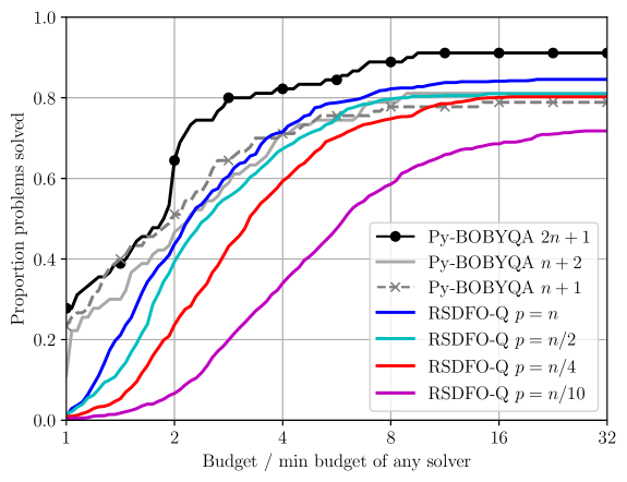
Solvers are compared using data profiles [27], showing the proportion of problem instances solved within a given number of evaluations in units of $(n+1)$ for problems in $\mathbb{R}^{n}$ (i.e. the cost of estimating a full gradient using finite differencing), and performance profiles [14], which plot the proportion of problem instances solved within a given ratio of the minimum evaluations required by any instance of any solver.

5.2 Medium-Scale Results

We first show results for medium-scale problems based on the ‘CFMR’ problem collection ( $n\approx 100$ ).⁶⁶6The 12hr runtime limit was not reached for any of these problem instances. In Figure 1, we compare Py-BOBYQA with $q\in\{n+1,n+2,2n+1\}$ interpolation points (i.e. linear or underdetermined quadratic interpolation models) against RSDFO-Q with $q=2p+1$ interpolation points, with subspace dimension $p\in\{n/10,n/4,n/2,n\}$ .

We see that the full-space method Py-BOBYQA is the best-performing algorithm, with larger numbers of interpolation points $q$ giving the best performance. Among the subspace methods, those with larger choices of $p$ achieve the best performance, aligning with the results in [9]. In particular (c.f. principles in Section 4), we see that RSDFO-Q with full blocks $p=n$ (and $q=2p+1$ interpolation points) achieves broadly comparable performance to Py-BOBYQA (worse than Py-BOBYQA with $q=2n+1$ points but better than $q=n+2$ points), while having the significant additional flexibility of working in a subspace of arbitrary dimension $p$ .

Refer to caption — (a) Data profile, $\tau=10^{-1}$ .

5.3 Large-Scale results

In Figure 2 we show the same results (based on total objective evaluations) as Figure 1, but for the large-scale test set ‘CR-large’ ( $n\approx 1000$ ). Here, we observe that Py-BOBYQA with quadratic models ( $q=2n+1$ and $q=n+2$ ) fail to solve any problems, as their significant per-iteration linear algebra costs⁷⁷7e.g. Model construction in each iteration of Py-BOBYQA with $q>n+1$ requires the solution of a $(q+n+1)\times(q+n+1)$ linear system. mean they hit the runtime limit quickly. The only Py-BOBYQA variant able to make progress uses linear models with $q=n+1$ . However, this method is outperformed by all variants of the subspace method RSDFO-Q (including with $p=n$ ). We find that medium-dimensional subspaces $p\in\{n/10,n/4\}$ (i.e. $p\approx 100$ and $p\approx 250$ ) are the best-performing variants.

For comparison, in Figure 3, we show data and performance profiles based on runtime to find a point with sufficient decrease. Among the variants of RSDFO-Q, we find that the low-dimensional variants $p\in\{n/10,n/100\}$ are the best-performing, at least initially. However, the increased robustness of the $p=n/4$ variant (accompanied by an increase in the per-iteration linear algebra cost) means it ultimately outperforms the $p=n/100$ variant.

6 Conclusion

We have provided the first second-order convergence result for a random subspace model-based DFO method, and shown that, compared to full space model-based DFO, these approaches can achieve a significant improvement in dimension dependence of the complexity bound, from $O(n^{11}\epsilon^{-3})$ evaluations to $\tilde{O}(n^{4.5}\epsilon^{-3})$ evaluations to find an $\epsilon$ -approximate second-order critical point for an $n$ -dimensional problem. This theory is relevant particularly when seeking low accuracy solutions or if the objective has low effective rank (i.e. low rank Hessians).

We then introduce a practical algorithm (RSDFO-Q) for general unconstrained model-based DFO in subspaces based on iterative construction of quadratic models in subspaces. This extends the practical method from [9], which was limited to linear models (and specialized to nonlinear least-squares problems). Numerical results compared to the state-of-the-art method Py-BOBYQA show that RSDFO-Q can solve problems of significantly higher dimension ( $n\approx 1000$ ), exploiting a significantly reduced per-iteration linear algebra cost, while RSDFO-Q with full-dimensional subspaces achieves comparable performance to Py-BOBYQA on medium-scale problems ( $n\approx 100$ ).

Interesting extensions of this approach would be to consider the case of stochastic function evaluations, similar to [16] for the first-order theory, and a practical comparison of RSDFO-Q for large language model fine-tuning problems, which typically have low effective rank [25].

Acknowledgement(s)

We acknowledge the use of the University of Oxford Advanced Research Computing (ARC) facility⁸⁸8http://dx.doi.org/10.5281/zenodo.22558 in carrying out this work.

Funding

LR was supported by the Australian Research Council Discovery Early Career Award DE240100006. CC was supported by the Hong Kong Innovation and Technology Commission (InnoHK CIMDA Project).

References

[1] S. Alarie, C. Audet, A.E. Gheribi, M. Kokkolaras, and S. Le Digabel, Two decades of blackbox optimization applications, EURO Journal on Computational Optimization 9 (2021), p. 100011.
[2] C. Audet and W. Hare, Derivative-Free and Blackbox Optimization, Springer Series in Operations Research and Financial Engineering, Springer, Cham, Switzerland, 2017.
[3] J. Blanchet, C. Cartis, M. Menickelly, and K. Scheinberg, Convergence rate analysis of a stochastic trust-region method via supermartingales, INFORMS Journal on Optimization 1 (2019), pp. 92–119.
[4] C. Cartis, J. Fiala, B. Marteau, and L. Roberts, Improving the flexibility and robustness of model-based derivative-free optimization solvers, ACM Transactions on Mathematical Software 45 (2019), pp. 1–41.
[5] C. Cartis, J. Fowkes, and Z. Shao, Randomised subspace methods for non-convex optimization, with applications to nonlinear least-squares, arXiv preprint arXiv:2211.09873 (2022).
[6] C. Cartis, X. Liang, E. Massart, and A. Otemissov, Learning the subspace of variation for global optimization of functions with low effective dimension, arXiv preprint arXiv:2401.17825 (2024).
[7] C. Cartis and A. Otemissov, A dimensionality reduction technique for unconstrained global optimization of functions with low effective dimensionality, Information and Inference: A Journal of the IMA 11 (2022), pp. 167–201.
[8] C. Cartis and L. Roberts, A derivative-free Gauss–Newton method, Mathematical Programming Computation 11 (2019), pp. 631–674.
[9] C. Cartis and L. Roberts, Scalable subspace methods for derivative-free nonlinear least-squares optimization, Mathematical Programming 199 (2023), pp. 461–524.
[10] C. Cartis, L. Roberts, and O. Sheridan-Methven, Escaping local minima with local derivative-free methods: A numerical investigation, Optimization 71 (2022), pp. 2343–2373.
[11] C. Cartis, Z. Shao, and E. Tansley, Random subspace cubic regularization methods, December (2024).
[12] Y. Chen, W. Hare, and A. Wiebe, Q-fully quadratic modeling and its application in a random subspace derivative-free method, Computational Optimization and Applications (2024).
[13] A.R. Conn, K. Scheinberg, and L.N. Vicente, Introduction to Derivative-Free Optimization, MPS-SIAM Series on Optimization, Society for Industrial and Applied Mathematics, Philadelphia, 2009.
[14] E.D. Dolan and J.J. Moré, Benchmarking optimization software with performance profiles, Mathematical Programming 91 (2002), pp. 201–213.
[15] K.J. Dzahini and S.M. Wild, Direct search for stochastic optimization in random subspaces with zeroth-, first-, and second-order convergence and expected complexity, arXiv preprint arXiv:2403.13320 (2024).
[16] K.J. Dzahini and S.M. Wild, Stochastic trust-region algorithm in random subspaces with convergence and expected complexity analyses, SIAM Journal on Optimization 34 (2024), pp. 2671–2699.
[17] M.J. Ehrhardt and L. Roberts, Inexact derivative-free optimization for bilevel learning, Journal of Mathematical Imaging and Vision 63 (2021), pp. 580–600.
[18] J. Fowkes, L. Roberts, and Á. Bűrmen, PyCUTEst: An open source Python package of optimization test problems, Journal of Open Source Software 7 (2022), p. 4377.
[19] R. Garmanjani, Trust-region methods without using derivatives: Worst case complexity and the nonsmooth case, Ph.D. diss., Universidade de Coimbra, 2015.
[20] N.I.M. Gould, D. Orban, and P.L. Toint, CUTEst: A constrained and unconstrained testing environment with safe threads for mathematical optimization, Computational Optimization and Applications 60 (2015), pp. 545–557.
[21] S. Gratton, C.W. Royer, L.N. Vicente, and Z. Zhang, Direct search based on probabilistic descent, SIAM Journal on Optimization 25 (2015), pp. 1515–1541.
[22] M. Kimiaei, A. Neumaier, and P. Faramarzi, New subspace method for unconstrained derivative-free optimization, ACM Transactions on Mathematical Software 49 (2023), pp. 1–28.
[23] D. Kozak, S. Becker, A. Doostan, and L. Tenorio, A stochastic subspace approach to gradient-free optimization in high dimensions, Computational Optimization and Applications 79 (2021), pp. 339–368.
[24] J. Larson, M. Menickelly, and S.M. Wild, Derivative-free optimization methods, Acta Numerica 28 (2019), pp. 287–404.
[25] S. Malladi, T. Gao, E. Nichani, A. Damian, J.D. Lee, D. Chen, and S. Arora, Fine-Tuning Language Models with Just Forward Passes, in 37th Conference on Neural Information Processing Systems (NeurIPS 2023). 2023.
[26] M. Menickelly, Avoiding geometry improvement in derivative-free model-based methods via randomization, arXiv preprint arXiv:2305.17336 (2023).
[27] J.J. Moré and S.M. Wild, Benchmarking derivative-free optimization algorithms, SIAM Journal on Optimization 20 (2009), pp. 172–191.
[28] M.J.D. Powell, Least Frobenius norm updating of quadratic models that satisfy interpolation conditions, Mathematical Programming 100 (2004), pp. 183–215.
[29] M.J.D. Powell, The BOBYQA algorithm for bound constrained optimization without derivatives, Tech. Rep. DAMTP 2009/NA06, University of Cambridge, 2009.
[30] L. Roberts and C.W. Royer, Direct search based on probabilistic descent in reduced spaces, SIAM Journal on Optimization 33 (2023).
[31] Z. Shao, On random embeddings and their application to optimisation, Ph.D. diss., University of Oxford, 2021.
[32] G. Ughi, V. Abrol, and J. Tanner, An empirical study of derivative-free-optimization algorithms for targeted black-box attacks in deep neural networks, Optimization and Engineering 23 (2022), pp. 1319–1346.
[33] D. van de Berg, N. Shan, and A. del Rio-Chanona, High-dimensional derivative-free optimization via trust region surrogates in linear subspaces, in Proceedings of the 34th European Symposium on Computer Aided Process Engineering / 15th International Symposium on Process Systems Engineering (ESCAPE34/PSE24). 2024.
[34] D.P. Woodruff, Sketching as a tool for numerical linear algebra, Foundations and Trends® in Theoretical Computer Science 10 (2014), pp. 1–157.
[35] P. Xie and Y.x. Yuan, A new two-dimensional model-based subspace method for large-scale unconstrained derivative-free optimization: 2D-MoSub, arXiv preprint arXiv:2309.14855 (2024).
[36] Z. Zhang, On derivative-free optimization methods, Ph.D. diss., Chinese Academy of Sciences, 2012.


$\displaystyle(1-\alpha)\\|\nabla f(\bm{x}_{k})\\|$	$\displaystyle\leq\\|P_{k}^{T}\nabla f(\bm{x}_{k})\\|\leq(1+\alpha)\\|\nabla f(\bm{x}_{k})\\|,$	(78a)
$\displaystyle(1-\alpha)\\|\bm{v}_{r}\\|$	$\displaystyle\leq\\|\hat{\bm{v}}_{r}\\|\leq(1+\alpha)\\|\bm{v}_{r}\\|,$	(78b)
$\displaystyle(1-\alpha)\\|\bm{v}_{i}+\bm{v}_{r}\\|$	$\displaystyle\leq\\|\hat{\bm{v}}_{i}+\hat{\bm{v}}_{r}\\|\leq(1+\alpha)\\|\bm{v}_{i}+\bm{v}_{r}\\|,\qquad\forall i=1,\ldots,r-1,$	(78c)
$\displaystyle(1-\alpha)\\|\bm{v}_{i}-\bm{v}_{r}\\|$	$\displaystyle\leq\\|\hat{\bm{v}}_{i}-\hat{\bm{v}}_{r}\\|\leq(1+\alpha)\\|\bm{v}_{i}-\bm{v}_{r}\\|,\qquad\forall i=1,\ldots,r-1,$	(78d)