Randomized block coordinate descent method for linear ill-posed problems

Qinian Jin Mathematical Scuences Institute, Australian National University, Canberra, ACT 2601, Australia [email protected] and Duo Liu School of Mathematics and Statistics, Beijing Jiaotong University, Beijing 100044, China [email protected]

Abstract.

Consider the linear ill-posed problems of the form $\sum_{i=1}^{b}A_{i}x_{i}=y$ , where, for each $i$ , $A_{i}$ is a bounded linear operator between two Hilbert spaces $X_{i}$ and ${\mathcal{Y}}$ . When $b$ is huge, solving the problem by an iterative method using the full gradient at each iteration step is both time-consuming and memory insufficient. Although randomized block coordinate decent (RBCD) method has been shown to be an efficient method for well-posed large-scale optimization problems with a small amount of memory, there still lacks a convergence analysis on the RBCD method for solving ill-posed problems. In this paper, we investigate the convergence property of the RBCD method with noisy data under either a priori or a posteriori stopping rules. We prove that the RBCD method combined with an a priori stopping rule yields a sequence that converges weakly to a solution of the problem almost surely. We also consider the early stopping of the RBCD method and demonstrate that the discrepancy principle can terminate the iteration after finite many steps almost surely. For a class of ill-posed problems with special tensor product form, we obtain strong convergence results on the RBCD method. Furthermore, we consider incorporating the convex regularization terms into the RBCD method to enhance the detection of solution features. To illustrate the theory and the performance of the method, numerical simulations from the imaging modalities in computed tomography and compressive temporal imaging are reported.

Key words and phrases:

linear ill-posed problems, randomized block coordinate descent method, convex regularization term, convergence, imaging

2010 Mathematics Subject Classification:

65J20, 65J22, 65J10, 94A08

1. Introduction

In this paper we consider linear ill-posed problems of the form

\sum_{i=1}^{b}A_{i}x_{i}=y,

(1)

where, for each $i=1,\cdots,b$ , $A_{i}:X_{i}\to{\mathcal{Y}}$ is a bounded linear operator between two real Hilbert spaces $X_{i}$ and ${\mathcal{Y}}$ . Ill-posed problems with such a form arise naturally from many applications in imaging. For example, coded aperture compressive temporal imaging (more details see Example 4.2 and [15]), a kind of large-scale snapshot compressive imaging [33], can be expressed by the following integral equation

(Ax)(s):=\int_{T}m(s,t)x(s,t)\mathop{}\!\mathrm{d}t=y(s),\quad s\in\Omega,

(2)

where $T=[t_{1},t_{2}]\subset[0,+\infty)$ , $\Omega$ is a bounded domains in 2-dimensional Euclidean spaces and $m$ is a bounded continuous mask function on $\Omega\times T$ , which ensures the forward operator $A$ is a bounded linear operator from $L^{2}(\Omega\times T)$ to $L^{2}(\Omega)$ . Decomposing the whole time domain $T$ into $b$ disjoint sub-domains $T_{1},\ldots,T_{b}$ , where for any $i=1,\ldots,b$ ,

T_{i}:=[\bar{t}_{i},\bar{t}_{i+1}],\quad\bar{t}_{i}:=\frac{t_{2}-t_{1}}{b}(i-1)+t_{1},

(3)

we denote the restriction of each function $x\in L^{2}(\Omega\times T)$ to $\Omega\times T_{i}$ as $x_{i}$ , i.e. $x_{i}:=x|_{\Omega\times T_{i}}$ and let

(A_{i}x_{i})(s):=\int_{T_{i}}m(s,t)x_{i}(s,t)\mathop{}\!\mathrm{d}t,\quad s\in\Omega,

(4)

then $A_{i}:L^{2}(\Omega\times T_{i})\rightarrow L^{2}(\Omega)$ is a bounded linear operator for each $i$ . Since

\int_{T}m(s,t)x(s,t)\mathop{}\!\mathrm{d}t=\sum_{i=1}^{b}\int_{T_{i}}m(s,t)x_{i}(s,t)\mathop{}\!\mathrm{d}t,

the above integral equation can be written as the form (1). For more examples, one may refer to the light field reconstruction from the focal stack [14, 32] and other imaging modalities such as spectral imaging [28] and full 3-D computed tomography [18]. In these examples, the sought solution can be separated into many films or frames naturally.

Let ${\mathcal{X}}:=X_{1}\times\cdots\times X_{b}$ be the product space of $X_{1},\cdots,X_{b}$ with the natural inner product inherited from those of $X_{i}$ and define $A:{\mathcal{X}}\to{\mathcal{Y}}$ by

Ax:=\sum_{i=1}^{b}A_{i}x_{i},\quad\forall x=(x_{1},\ldots,x_{b})\in{\mathcal{X}}.

(5)

Then, (1) can be equivalently stated as $Ax=y$ . Throughout the paper we assume that (1) has a solution, i.e. $y\in\mbox{Ran}(A)$ , the range of $A$ . In practical applications, instead of the exact data $y$ we can only acquire a noisy data $y^{\delta}$ satisfying

\|y-y^{\delta}\|\leq\delta,

where $\delta>0$ is the noise level. How to stably reconstruct an approximate solution of ill-posed problems described by (1) using noisy data $y^{\delta}$ is a central topic in computational inverse problems. In this situation, the regularization techniques should be used and various regularization methods have been developed in the literature ([6]).

In this paper we will exploit the decomposition structure of the equation (1) to develop a randomized block coordinate descent method for solving ill-posed linear problems. The researches on the block coordinate descent method in the literature mainly focus on solving large scale well-posed optimization problems ([17, 19, 22, 24, 25, 26, 27, 30]). For the unconstrained minimization problem

\displaystyle\min_{(x_{1},\cdots,x_{b})\in{\mathcal{X}}}f(x_{1},\cdots,x_{b})

(6)

with ${\mathcal{X}}=X_{1}\times\cdots\times X_{b}$ , where $f:{\mathcal{X}}\to{\mathbb{R}}$ is a continuous differentiable function, the block coordinate descent method updates $x_{k+1}:=(x_{k+1,1},\cdots,x_{k+1,b})$ from $x_{k}:=(x_{k,1},\cdots,x_{k,b})$ by selecting an index $i_{k}$ from $\{1,\cdots,b\}$ and uses the partial gradient $\nabla_{i_{k}}f(x_{k})$ of $f$ at $x_{k}$ to update the component $x_{k+1,i_{k}}$ of $x_{k+1}$ and leave other components unchanged; more precisely, we have the updating formula

x_{k+1,i}=\begin{cases}x_{k,i_{k}}-\gamma\nabla_{i_{k}}f(x_{k}),&\text{if}\ i=i_{k},\\ x_{k,i},&\text{otherwise},\end{cases}

(7)

where $\gamma$ is the step size. The index $i_{k}$ can be selected in various ways, either in a cyclic fashion or in a random manner. By applying the block coordinate descent method (7) to solve (6) with $f$ given by

\displaystyle f(x_{1},\cdots,x_{b})=\frac{1}{2}\left\|\sum_{i=1}^{b}A_{i}x_{i}-y^{\delta}\right\|^{2},

(8)

it leads to the iterative method

x_{k+1,i}^{\delta}=\begin{cases}x_{k,i_{k}}^{\delta}-\gamma A^{*}_{i_{k}}(Ax_{k}^{\delta}-y^{\delta}),&\text{if}\ i=i_{k},\\ x_{k,i}^{\delta},&\text{otherwise}\end{cases}

(9)

for solving ill-posed linear problem (1) using noisy data $y^{\delta}$ , where $A_{i}^{*}:{\mathcal{Y}}\to X_{i}$ denotes the adjoint of $A_{i}$ for each $i$ and the superscript “ $\delta$ ” on all iterates is used to indicate their dependence on the noisy data.

The method (9) can also be motivated from the Landweber iteration

x_{k+1}^{\delta}=x_{k}^{\delta}-\gamma A^{*}(Ax_{k}^{\delta}-y^{\delta}),

(10)

which is one of the most prominent regularization methods for solving ill-posed problems, where $\gamma$ is the step-size and $A^{*}:{\mathcal{Y}}\to{\mathcal{X}}$ is the adjoint of $A$ . Note that, with the operator $A$ defined by (5), we have

A^{*}z=\left(A_{1}^{*}z,\cdots,A_{b}^{*}z\right),\quad\forall z\in{\mathcal{Y}}.

Thus, updating $x_{k+1}^{\delta}$ from $x_{k}^{\delta}$ by (10) needs calculating $A_{i}^{*}(Ax_{k}^{\delta}-y^{\delta})$ for all $i=1,\cdots,b$ . If $b$ is huge, applying the method (10) to solve the equation (1) is both time-consuming and memory insufficient. To resolve these issues, it is natural to calculate only one component of $A^{*}(Ax_{k}^{\delta}-y^{\delta})$ and use it to update the corresponding component of $x_{k+1}^{\delta}$ and keep other components fixed. This leads again to the block coordinate descent method (9) for solving (1).

The block coordinate descent method and its variants for large scale well-posed optimization problems have been analyzed extensively, and all the established convergence results require either the objective function to be strongly convex or the convergence is established in terms of the objective value. However, these results are not applicable to the method (9) for ill-posed problems because the corresponding objective function (8) is not strongly convex, and moreover, due to the ill-posedness of the underlying problem, convergence on objective value does not imply any result on the iterates directly. Therefore, new analysis is required for understanding the method (9) for ill-posed problems.

In [21] the block coordinate descent method (9) was considered with the index $i_{k}$ selected in a cyclic fashion, i.e. $i_{k}=(k\ \text{mod}\ b)+1$ . The regularization property of the corresponding method was only established for a specific class of linear ill-posed problems in which the forward operator $A$ is assumed a particular tensor product form; more precisely, the ill-posed linear system of the form

\displaystyle\sum_{i=1}^{b}v_{li}Kx_{i}=y_{l},\quad l=1,\cdots,d,

(11)

was considered in [21], where $K:X\to Y$ is a bounded linear operator between two real Hilbert spaces $X$ and $Y$ and $V=(v_{li})$ is a $d\times b$ matrix with full column rank. Clearly this problem can be cast into the form (1) if we take $X_{i}=X$ for each $i$ , ${\mathcal{Y}}=Y^{d}$ , the $d$ -fold Cartesian product of $Y$ , and define $A_{i}:X\to{\mathcal{Y}}$ by

A_{i}z=(v_{1i}Kz,\cdots,v_{di}Kz),\quad z\in X

for each $i=1,\cdots,b$ . The problem formulation (11), however, seems too specific to cover interesting problems arising from practical applications. How to establish the regularization property of this cyclic block coordinate descent method for ill-posed problem (1) in its full generality remains a challenging open question.

Instead of using a deterministic cyclic order, in this paper we will consider a randomized block coordinate descent method, i.e. the method (9) with $i_{k}$ being selected from $\{1,\cdots,b\}$ uniformly at random. We will investigate the convergence behavior of the iterates for the ill-posed linear problem (1) with general forward operator $A$ . Note that in the method (9) the definition of $x_{k+1}^{\delta}$ involves $r_{k}^{\delta}:=Ax_{k}^{\delta}-y^{\delta}$ . If this quantity is required to be calculated directly at each iteration step, then the advantages of the method will be largely reduced. Fortunately, this quantity can be calculated in a simple recursive way. Indeed, by the definition of $x_{k+1}^{\delta}$ we have

	$\displaystyle r_{k+1}^{\delta}$	$\displaystyle=\sum_{i=1}^{b}A_{i}x_{k+1}^{\delta}-y^{\delta}=\sum_{i\neq i_{k}}A_{i}x_{k+1,i}^{\delta}+A_{i_{k}}x_{k+1,i_{k}}^{\delta}-y^{\delta}$
		$\displaystyle=\sum_{i\neq i_{k}}A_{i}x_{k,i}^{\delta}+A_{i_{k}}x_{k,i_{k}}^{\delta}+A_{i_{k}}(x_{k+1,i_{k}}^{\delta}-x_{k,i_{k}}^{\delta})-y^{\delta}$
		$\displaystyle=Ax_{k}^{\delta}-y^{\delta}+A_{i_{k}}(x_{k+1,i_{k}}^{\delta}-x_{k,i_{k}}^{\delta})$
		$\displaystyle=r_{k}^{\delta}+A_{i_{k}}(x_{k+1,i_{k}}^{\delta}-x_{k,i_{k}}^{\delta}).$

Therefore, we can formulate our randomized block coordinate descent (RBCD) method into the following equivalent form which is convenient for numerical implementation.

Algorithm 1 (RBCD method for ill-posed problems).

Pick an initial guess $x_{0}\in{\mathcal{X}}$ , set $x_{0}^{\delta}:=x_{0}$ and calculate $r_{0}^{\delta}:=Ax_{0}^{\delta}-y^{\delta}$ . Choose a suitable step size $\gamma>0$ . For all integers $k\geq 0$ do the following:

(i)

Pick an index $i_{k}\in\{1,\cdots,b\}$ randomly via the uniform distribution;
(ii)

Update $x_{k+1}^{\delta}$ by setting $x_{k+1,i}^{\delta}=x_{k,i}^{\delta}$ for $i\neq i_{k}$ and

$x_{k+1,i_{k}}^{\delta}=x_{k,i_{k}}^{\delta}-\gamma A_{i_{k}}^{*}r_{k}^{\delta};$
(iii)

Calculate $r_{k+1}^{\delta}=r_{k}^{\delta}+A_{i_{k}}(x_{k+1,i_{k}}^{\delta}-x_{k,i_{k}}^{\delta})$ .

In this paper we present a convergence analysis on Algorithm 1 by deriving the stability estimate and establishing the regularization property. For the equation (1) in the general form, we obtain a weak convergence result and for a particular tensor product form as studied in [21] we establish the strong convergence result. Moreover, we also consider the early stopping of Algorithm 1 and demonstrate that the discrepancy principle can terminate the iteration after finite many steps almost surely. Note that, Algorithm 1 does not incorporate a priori available information on the feature of the sought solution. In case the sought solution has some special feature, such as non-negativity, sparsity and piece-wise constancy, Algorithm 1 may not be efficient enough to produce satisfactory approximate solutions. In order to resolve this issue, we further extend Algorithm 1 by incorporating into it a convex regularization term which is selected to capture the desired feature. For a detailed description of this extended algorithm, please refer to Algorithm 3 for which we will provide a convergence analysis.

It should be pointed out that the RBCD method is essentially different from the Landweber-Kaczmarz method and its stochastic version which have been studied in [8, 10, 11, 12, 13]. The Landweber-Kaczmarz method relies on decomposing the data into many blocks of small size, while our RBCD method makes use of the block structure of the sought solutions.

This paper is organized as follows. In Section 2 we consider Algorithm 1 by proving various convergence results and investigating the discrepancy principle as an early stopping rule. In Section 3 we consider an extension of Algorithm 1 by incorporating a convex regularization term into it so that the special feature of sought solutions can be detected. Finally in Section 4 we provide numerical simulations to test the performance of our proposed methods.

2. Convergence analysis

In this section we consider Algorithm 1. We first establish a stability estimate, and prove a weak convergence result when the method is terminated by an a priori stopping rule. We then investigate the discrepancy principle and demonstrate that it can terminate the iteration in finite many steps almost surely. When the forward operator $A$ has a particular tensor product form as used in [21], we further show that strong convergence can be guaranteed.

Note that, once $x_{0}\in{\mathcal{X}}$ and $\gamma$ are fixed, the sequence $\{x_{k}^{\delta}\}$ is completely determined by the sample path $\{i_{0},i_{1},\cdots\}$ ; changing the sample path can result in a different iterative sequence and thus $\{x_{k}^{\delta}\}$ is a random sequence. Let ${\mathcal{F}}_{0}=\emptyset$ and, for each integer $k\geq 1$ , let ${\mathcal{F}}_{k}$ denote the $\sigma$ -algebra generated by the random variables $i_{l}$ for $0\leq l<k$ . Then $\{{\mathcal{F}}_{k}:k\geq 0\}$ form a filtration which is natural to Algorithm 1. Let $\mathbb{E}$ denote the expectation associated with this filtration, see [4]. The tower property of conditional expectation

\mathbb{E}[\mathbb{E}[\phi|{\mathcal{F}}_{k}]]=\mathbb{E}[\phi]\quad\mbox{ for any random variable }\phi

will be frequently used.

2.1. Stability estimate

Let $\{x_{k}\}$ denote the iterative sequence produced by Algorithm 1 with $y^{\delta}$ replaced by the exact data $y$ . By definition it is easy to see that, for any fixed integer $k\geq 0$ , along any sample path there holds $\|x_{k}^{\delta}-x_{k}\|\to 0$ as $\delta\to 0$ and hence $\mathbb{E}[\|x_{k}^{\delta}-x_{k}\|^{2}]\to 0$ as $\delta\to 0$ . The following result gives a more precise stability estimate.

Lemma 2.1.

Consider Algorithm 1 and assume $0<\gamma\leq 2/\|A\|^{2}$ . Then, along any sample path there holds

\displaystyle\|A(x_{k}^{\delta}-x_{k})-y^{\delta}+y\|\leq\delta

(12)

for all integers $k\geq 0$ . Furthermore

\displaystyle\mathbb{E}[\|x_{k}^{\delta}-x_{k}\|^{2}]\leq\frac{2\gamma}{b}k\delta^{2}

(13)

for all $k\geq 0$ .

Proof.

Let $u_{k}^{\delta}:=x_{k}^{\delta}-x_{k}$ for all integers $k\geq 0$ . It follows from the definition of $x_{k+1}^{\delta}$ and $x_{k+1}$ that

\displaystyle u_{k+1,i}^{\delta}=\left\{\begin{array}[]{lll}u_{k,i}^{\delta}&\mbox{ if }i\neq i_{k},\\[4.73611pt] u_{k,i_{k}}^{\delta}-\gamma A_{i_{k}}^{*}(Au_{k}^{\delta}-y^{\delta}+y)&\mbox{ if }i=i_{k}.\end{array}\right.

Thus

	$\displaystyle Au_{k+1}^{\delta}-y^{\delta}+y$	$\displaystyle=\sum_{i\neq i_{k}}A_{i}u_{k+1,i}^{\delta}+A_{i_{k}}u_{k+1,i_{k}}^{\delta}-y^{\delta}+y$
		$\displaystyle=\sum_{i=1}^{b}A_{i}u_{k,i}^{\delta}-\gamma A_{i_{k}}A_{i_{k}}^{*}(Au_{k}^{\delta}-y^{\delta}+y)-y^{\delta}+y$
		$\displaystyle=(I-\gamma A_{i_{k}}A_{i_{k}}^{*})(Au_{k}^{\delta}-y^{\delta}+y).$

Since $\|A_{i_{k}}\|\leq\|A\|$ and $0<\gamma\leq 2/\|A\|^{2}$ , we have $\|I-\gamma A_{i_{k}}A_{i_{k}}^{*}\|\leq 1$ and thus

\|Au_{k+1}^{\delta}-y^{\delta}+y\|\leq\|I-\gamma A_{i_{k}}A_{i_{k}}^{*}\|\|Au_{k}^{\delta}-y^{\delta}+y\|\leq\|Au_{k}^{\delta}-y^{\delta}+y\|.

Consequently

\displaystyle\|Au_{k+1}^{\delta}-y^{\delta}+y\|\leq\|Au_{0}^{\delta}-y^{\delta}+y\|=\|y^{\delta}-y\|\leq\delta

which shows (12).

To derive (13), we note that

	$\displaystyle\\|u_{k+1}^{\delta}\\|^{2}$	$\displaystyle=\sum_{i\neq i_{k}}\\|u_{k+1,i}^{\delta}\\|^{2}+\\|u_{k+1,i_{k}}^{\delta}\\|^{2}$
		$\displaystyle=\sum_{i\neq i_{k}}\\|u_{k,i}^{\delta}\\|^{2}+\\|u_{k,i_{k}}^{\delta}-\gamma A_{i_{k}}^{*}(Au_{k}^{\delta}-y^{\delta}+y)\\|^{2}$
		$\displaystyle=\sum_{i\neq i_{k}}\\|u_{k,i}^{\delta}\\|^{2}+\\|u_{k,i_{k}}^{\delta}\\|^{2}+\gamma^{2}\\|A_{i_{k}}^{*}(Au_{k}^{\delta}-y^{\delta}+y)\\|^{2}$
		$\displaystyle\quad\,-2\gamma\langle u_{k,i_{k}}^{\delta},A_{i_{k}}^{*}(Au_{k}^{\delta}-y^{\delta}+y)\rangle$
		$\displaystyle=\\|u_{k}^{\delta}\\|^{2}+\gamma^{2}\\|A_{i_{k}}^{*}(Au_{k}^{\delta}-y^{\delta}+y)\\|^{2}$
		$\displaystyle\quad\,-2\gamma\langle A_{i_{k}}u_{k,i_{k}}^{\delta},Au_{k}^{\delta}-y^{\delta}+y\rangle.$

Taking the conditional expectation gives

	$\displaystyle\mathbb{E}[\\|u_{k+1}^{\delta}\\|^{2}\|{\mathcal{F}}_{k}]$
	$\displaystyle=\\|u_{k}^{\delta}\\|^{2}+\frac{\gamma^{2}}{b}\sum_{i=1}^{b}\\|A_{i}^{*}(Au_{k}^{\delta}-y^{\delta}+y)\\|^{2}-\frac{2\gamma}{b}\left\langle\sum_{i=1}^{b}A_{i}u_{k,i}^{\delta},Au_{k}^{\delta}-y^{\delta}+y\right\rangle$
	$\displaystyle=\\|u_{k}^{\delta}\\|^{2}+\frac{\gamma^{2}}{b}\\|A^{*}(Au_{k}^{\delta}-y^{\delta}+y)\\|^{2}-\frac{2\gamma}{b}\left\langle Au_{k}^{\delta},Au_{k}^{\delta}-y^{\delta}+y\right\rangle$
	$\displaystyle\leq\\|u_{k}^{\delta}\\|^{2}+\frac{\gamma^{2}\\|A\\|^{2}}{b}\\|Au_{k}^{\delta}-y^{\delta}+y\\|^{2}-\frac{2\gamma}{b}\\|Au_{k}^{\delta}-y^{\delta}+y\\|^{2}$
	$\displaystyle\quad\,-\frac{2\gamma}{b}\langle y^{\delta}-y,Au_{k}^{\delta}-y^{\delta}+y\rangle$
	$\displaystyle\leq\\|u_{k}^{\delta}\\|^{2}-\frac{1}{b}(2-\gamma\\|A\\|^{2})\gamma\\|Au_{k}^{\delta}-y^{\delta}+y\\|^{2}+\frac{2\gamma}{b}\delta\\|Au_{k}^{\delta}-y^{\delta}+y\\|.$

By using $0<\gamma\leq 2/\|A\|^{2}$ and (12), we further obtain

\displaystyle\mathbb{E}[\|u_{k+1}^{\delta}\|^{2}|{\mathcal{F}}_{k}]\leq\|u_{k}^{\delta}\|^{2}+\frac{2\gamma}{b}\delta\|Au_{k}^{\delta}-y^{\delta}+y\|\leq\|u_{k}^{\delta}\|^{2}+\frac{2\gamma}{b}\delta^{2}.

Consequently, by taking the full expectation and using the tower property of conditional expectation, we can obtain

\displaystyle\mathbb{E}\left[\|u_{k+1}^{\delta}\|^{2}\right]=\mathbb{E}\left[\mathbb{E}\left[\|u_{k+1}^{\delta}\|^{2}|{\mathcal{F}}_{k}\right]\right]\leq\mathbb{E}\left[\|u_{k}^{\delta}\|^{2}\right]+\frac{2\gamma\delta^{2}}{b}.

Based on this inequality and the fact $u_{0}^{\delta}=0$ , we can use an induction argument to complete the proof of (13) immediately. ∎

2.2. Weak convergence

Our goal is to investigate the approximation behavior of $x_{k}^{\delta}$ to a solution of $Ax=y$ . Because of Lemma 2.1, we now focus our consideration on the sequence $\{x_{k}\}$ defined by Algorithm 1 using exact data.

Lemma 2.2.

Assume $0<\gamma<2/\|A\|^{2}$ . Then for any solution $\bar{x}$ of (1) there holds

\displaystyle\mathbb{E}[\|x_{k+1}-\bar{x}\|^{2}|{\mathcal{F}}_{k}]\leq\|x_{k}-\bar{x}\|^{2}-c_{0}\|Ax_{k}-y\|^{2}

(14)

for all integers $k\geq 0$ , where $c_{0}:=(2-\gamma\|A\|^{2})\gamma/b>0$ .

Proof.

Let $\bar{x}_{i}$ denote the $i$ -th component of $\bar{x}$ , i.e. $\bar{x}=(\bar{x}_{1},\cdots,\bar{x}_{b})$ . By the definition of $x_{k+1}$ and the polarization identity, we have

	$\displaystyle\\|x_{k+1}-\bar{x}\\|^{2}$	$\displaystyle=\sum_{i\neq i_{k}}\\|x_{k+1,i}-\bar{x}_{i}\\|^{2}+\\|x_{k+1,i_{k}}-\bar{x}_{i_{k}}\\|^{2}$
		$\displaystyle=\sum_{i\neq i_{k}}\\|x_{k,i}-\bar{x}_{i}\\|^{2}+\\|x_{k,i_{k}}-\bar{x}_{i_{k}}-\gamma A_{i_{k}}^{*}(Ax_{k}-y)\\|^{2}$
		$\displaystyle=\sum_{i\neq i_{k}}\\|x_{k,i}-\bar{x}_{i}\\|^{2}+\\|x_{k,i_{k}}-\bar{x}_{i_{k}}\\|^{2}+\gamma^{2}\\|A_{i_{k}}^{*}(Ax_{k}-y)\\|^{2}$
		$\displaystyle\quad\,-2\gamma\langle x_{k,i_{k}}-\bar{x}_{i_{k}},A_{i_{k}}^{*}(Ax_{k}-y)\rangle$
		$\displaystyle=\\|x_{k}-\bar{x}\\|^{2}+\gamma^{2}\\|A_{i_{k}}^{*}(Ax_{k}-y)\\|^{2}$
		$\displaystyle\quad\,-2\gamma\langle A_{i_{k}}(x_{k,i_{k}}-\bar{x}_{i_{k}}),Ax_{k}-y\rangle.$

Taking the conditional expectation and using $A\bar{x}=y$ , we can obtain

	$\displaystyle\mathbb{E}[\\|x_{k+1}-\bar{x}\\|^{2}\|{\mathcal{F}}_{k}]$
	$\displaystyle=\\|x_{k}-\bar{x}\\|^{2}+\frac{\gamma^{2}}{b}\sum_{i=1}^{b}\\|A_{i}^{*}(Ax_{k}-y)\\|^{2}-\frac{2\gamma}{b}\sum_{i=1}^{b}\langle A_{i}(x_{k,i}-\bar{x}_{i}),Ax_{k}-y\rangle$
	$\displaystyle=\\|x_{k}-\bar{x}\\|^{2}+\frac{\gamma^{2}}{b}\\|A^{*}(Ax_{k}-y)\\|^{2}-\frac{2\gamma}{b}\langle A(x_{k}-\bar{x}),Ax_{k}-y\rangle$
	$\displaystyle\leq\\|x_{k}-\bar{x}\\|^{2}+\frac{\gamma^{2}\\|A\\|^{2}}{b}\\|Ax_{k}-y\\|^{2}-\frac{2\gamma}{b}\\|Ax_{k}-y\\|^{2}$

which shows (14). ∎

To proceed further, we need the following Doob’s martingale convergence theorem ([4]).

Proposition 2.3.

Let $\{U_{k}\}$ be a sequence of nonnegative random variables in a probability space that is a supermartingale with respect to a filtration $\{{\mathcal{F}}_{k}\}$ , i.e.

\mathbb{E}[U_{k+1}|{\mathcal{F}}_{k}]\leq U_{k},\quad\forall k.

Then $\{U_{k}\}$ converges almost surely to a nonnegative random variable $U$ with finite expectation.

Based on Proposition 2.3, we next prove the almost sure weak convergence of $\{x_{k}\}$ . We need ${\mathcal{X}}$ to be separable in the sense that ${\mathcal{X}}$ has a countable dense subset.

Theorem 2.4.

Consider the sequence $\{x_{k}\}$ defined by Algorithm 1 using exact data. Assume that ${\mathcal{X}}$ is separable and $0<\gamma<2/\|A\|^{2}$ , then $\{x_{k}\}$ converges weakly to a random solution $\bar{x}$ of (1) almost surely.

Proof.

Let $S$ denote the set of solutions of (1). According to Lemma 2.2, we have for any solution $z\in S$ that

\mathbb{E}[\|x_{k+1}-z\|^{2}|{\mathcal{F}}_{k}]\leq\|x_{k}-z\|^{2},\quad\forall k

which means $\{\|x_{k}-z\|^{2}\}$ is a supermartingale. Thus, we may use Proposition 2.3 to conclude that the event

\Omega_{z}:=\left\{\lim_{k\to\infty}\|x_{k}-z\|\mbox{ exists and is finite}\right\}

has probability one. We now strengthen this result by showing that there is an event $\Omega_{1}$ of probability one such that, for any $\tilde{z}\in S$ and any sample path $\omega\in\Omega_{1}$ , the limit $\lim_{k\to\infty}\|x_{k}(\omega)-\tilde{z}\|$ exists. We adapt the arguments in [2, 5]. By the separability of ${\mathcal{X}}$ , we can find a countable set $C\subset S$ such that $C$ is dense in $S$ . Let

\Omega_{1}:=\bigcap_{z\in C}\Omega_{z}.

Since $\mathbb{P}(\Omega_{z})=1$ for each $z\in C$ and $C$ is countable, we have $\mathbb{P}(\Omega_{1})=1$ . Let $\tilde{z}\in S$ be any point. Then there is a sequence $\{z_{l}\}\subset C$ such that $z_{l}\to\tilde{z}$ as $l\to\infty$ . For any sample path $\omega\in\Omega_{1}$ we have by the triangle inequality that

-\|z_{l}-\tilde{z}\|\leq\|x_{k}(\omega)-\tilde{z}\|-\|x_{k}(\omega)-z_{l}\|\leq\|z_{l}-\tilde{z}\|.

Thus

	$\displaystyle-\\|z_{l}-\tilde{z}\\|$	$\displaystyle\leq\liminf_{k\to\infty}\left\{\\|x_{k}(\omega)-\tilde{z}\\|-\\|x_{k}(\omega)-z_{l}\\|\right\}$
		$\displaystyle\leq\limsup_{k\to\infty}\left\{\\|x_{k}(\omega)-\tilde{z}\\|-\\|x_{k}(\omega)-z_{l}\\|\right\}$
		$\displaystyle\leq\\|z_{l}-\tilde{z}\\|.$

Since $\omega\in\Omega_{1}\subset\Omega_{z_{l}}$ , $\lim_{k\to\infty}\|x_{k}(\omega)-z_{l}\|$ exists. Thus, by the properties of $\liminf$ and $\limsup$ we have

	$\displaystyle-\\|z_{l}-\tilde{z}\\|$	$\displaystyle\leq\liminf_{k\to\infty}\\|x_{k}(\omega)-\tilde{z}\\|-\lim_{k\to\infty}\\|x_{k}(\omega)-z_{l}\\|$
		$\displaystyle\leq\limsup_{k\to\infty}\\|x_{k}(\omega)-\tilde{z}\\|-\lim_{k\to\infty}\\|x_{k}(\omega)-z_{l}\\|$
		$\displaystyle\leq\\|z_{l}-\tilde{z}\\|.$

This implies that both $\liminf_{k\to\infty}\|x_{k}(\omega)-\tilde{z}\|$ and $\limsup_{k\to\infty}\|x_{k}(\omega)-\tilde{z}\|$ are finite with

0\leq\limsup_{k\to\infty}\|x_{k}(\omega)-\tilde{z}\|-\liminf_{k\to\infty}\|x_{k}(\omega)-\tilde{z}\|\leq 2\|z_{l}-\tilde{z}\|.

Letting $l\to\infty$ shows that

\liminf_{k\to\infty}\|x_{k}(\omega)-\tilde{z}\|=\limsup_{k\to\infty}\|x_{k}(\omega)-\tilde{z}\|

and hence $\lim_{k\to\infty}\|x_{k}(\omega)-\tilde{z}\|$ exists and is finite for every $\omega\in\Omega_{1}$ and $\tilde{z}\in S$ .

Next we use Lemma 2.2 again to obtain for any $z\in S$ that

\mathbb{E}[\|x_{k+1}-z\|^{2}]\leq\mathbb{E}[\|x_{k}-z\|^{2}]-c_{0}\mathbb{E}[\|Ax_{k}-y\|^{2}]

which implies that

\mathbb{E}\left[\sum_{k=0}^{\infty}\|Ax_{k}-y\|^{2}\right]=\sum_{k=0}^{\infty}\mathbb{E}[\|Ax_{k}-y\|^{2}]\leq\frac{\|x_{0}-z\|^{2}}{c_{0}}<\infty.

Consequently, the event

\displaystyle\Omega_{2}:=\left\{\sum_{k=0}^{\infty}\|Ax_{k}-y\|^{2}<\infty\right\}

(15)

has probability one. Let $\Omega_{0}:=\Omega_{1}\cap\Omega_{2}$ . Then $\mathbb{P}(\Omega_{0})=1$ . Note that along any sample path in $\Omega_{0}$ we have $\{\|x_{k}-z\|\}$ is convergent for any $z\in S$ and

\sum_{k=0}^{\infty}\|Ax_{k}-y\|^{2}<\infty

which implies $\|Ax_{k}-y\|\to 0$ as $k\to\infty$ . The convergence of $\{\|x_{k}-z\|\}$ implies that $\{x_{k}\}$ is bounded and hence it has a weakly convergent subsequence $\{x_{k_{l}}\}$ such that $x_{k_{l}}\rightharpoonup\bar{x}$ as $l\to\infty$ for some $\bar{x}\in{\mathcal{X}}$ , where “ $\rightharpoonup$ ” denotes the weak convergence. Since $Ax_{k}\to y$ , we must have $A\bar{x}=y$ , i.e. $\bar{x}\in S$ and consequently $\|x_{k}-\bar{x}\|$ converges. We now show that $x_{k}\rightharpoonup\bar{x}$ for the whole sequence $\{x_{k}\}$ . It suffices to show that $\bar{x}$ is the unique weak cluster point of $\{x_{k}\}$ . Let $x^{*}$ be any cluster point of $\{x_{k}\}$ . Then there is another subsequence $\{x_{n_{l}}\}$ of $\{x_{k}\}$ such that $x_{n_{l}}\rightharpoonup x^{*}$ . From the above argument we also have $x^{*}\in S$ and thus $\{\|x_{k}-x^{*}\|\}$ is convergent. Noting the identity

\langle x_{k},x^{*}-\bar{x}\rangle=\|x_{k}-\bar{x}\|^{2}-\|x_{k}-x^{*}\|^{2}-\|\bar{x}\|^{2}+\|x^{*}\|^{2}.

Since both $\{\|x_{k}-\bar{x}\|\}$ and $\{\|x_{k}-x^{*}\|\}$ are convergent, we can conclude that $\lim_{k\to\infty}\langle x_{k},x^{*}-\bar{x}\rangle$ exists. Therefore

	$\displaystyle\lim_{k\to\infty}\langle x_{k},x^{*}-\bar{x}\rangle$	$\displaystyle=\lim_{l\to\infty}\langle x_{k_{l}},x^{}-\bar{x}\rangle=\langle\bar{x},x^{}-\bar{x}\rangle,$
	$\displaystyle\lim_{k\to\infty}\langle x_{k},x^{*}-\bar{x}\rangle$	$\displaystyle=\lim_{l\to\infty}\langle x_{n_{l}},x^{}-\bar{x}\rangle=\langle x^{},x^{*}-\bar{x}\rangle$

and thus $\langle\bar{x},x^{*}-\bar{x}\rangle=\langle x^{*},x^{*}-\bar{x}\rangle$ , i.e. $\|x^{*}-\bar{x}\|^{2}=0$ and hence $x^{*}=\bar{x}$ . The proof is complete. ∎

Remark 2.5.

Theorem 2.4 shows that there is an event $\Omega_{0}$ of probability one and a random vector $\bar{x}$ such that $A\bar{x}=y$ almost surely and $x_{k}\rightharpoonup\bar{x}$ along every sample path in $\Omega_{0}$ . Let $x^{\dagger}$ denote the unique $x_{0}$ -minimum-norm solution of $Ax=y$ . We would like to point out that $\bar{x}=x^{\dagger}$ almost surely if $\{x_{k}\}$ is uniformly bounded in the sense that

\displaystyle\mbox{there is a constant }C\mbox{ such that }\|x_{k}\|\leq C\mbox{ for all }k\mbox{ almost surely}.

(16)

To see this, we first claim that

\displaystyle\mathbb{E}[\langle x_{k}-x_{0},\bar{x}-x^{\dagger}\rangle]=0,\quad\forall k.

(17)

Indeed this is trivial for $k=0$ . Assume it is true for some $k\geq 0$ . Then, by the definition of $x_{k+1}$ , we have

	$\displaystyle\langle x_{k+1}-x_{0},\bar{x}-x^{\dagger}\rangle$	$\displaystyle=\langle x_{k}-x_{0},\bar{x}-x^{\dagger}\rangle-\gamma\langle A_{i_{k}}^{*}(Ax_{k}-y),\bar{x}_{i_{k}}-x_{i_{k}}^{\dagger}\rangle$
		$\displaystyle=\langle x_{k}-x_{0},\bar{x}-x^{\dagger}\rangle-\gamma\langle Ax_{k}-y,A_{i_{k}}(\bar{x}_{i_{k}}-x_{i_{k}}^{\dagger})\rangle.$

Thus

	$\displaystyle\mathbb{E}[\langle x_{k+1}-x_{0},\bar{x}-x^{\dagger}\rangle\|{\mathcal{F}}_{k}]$	$\displaystyle=\langle x_{k}-x_{0},\bar{x}-x^{\dagger}\rangle-\frac{\gamma}{b}\left\langle Ax_{k}-y,\sum_{i=1}^{b}A_{i}(\bar{x}_{i}-x_{i}^{\dagger})\right\rangle$
		$\displaystyle=\langle x_{k}-x_{0},\bar{x}-x^{\dagger}\rangle-\frac{\gamma}{b}\langle Ax_{k}-y,A(\bar{x}-x^{\dagger})\rangle$
		$\displaystyle=\langle x_{k}-x_{0},\bar{x}-x^{\dagger}\rangle$

because $A\bar{x}=y=Ax^{\dagger}$ almost surely. Consequently, by taking the full expectation and using the induction hypothesis we can obtain $\mathbb{E}[\langle x_{k+1}-x_{0},\bar{x}-x^{\dagger}\rangle]=0$ and the claim (17) is proved.

Under the condition (16), we have

|\langle x_{k}-x_{0},\bar{x}-x^{\dagger}\rangle|\leq\|x_{k}-x_{0}\|\|\bar{x}-x^{\dagger}\|\leq(C+\|x_{0}\|)\|\bar{x}-x^{\dagger}\|.

Since $x_{k}\rightharpoonup\bar{x}$ almost surely, by using the weak lower semi-continuity of norms and the Fatou lemma we can obtain from Lemma 2.2 that

	$\displaystyle\mathbb{E}[\\|\bar{x}-x^{\dagger}\\|^{2}]$	$\displaystyle\leq\mathbb{E}\left[\liminf_{k\to\infty}\\|x_{k}-x^{\dagger}\\|^{2}\right]\leq\liminf_{k\to\infty}\mathbb{E}[\\|x_{k}-x^{\dagger}\\|^{2}]$
		$\displaystyle\leq\\|x_{0}-x^{\dagger}\\|^{2}<\infty$

and thus

\mathbb{E}[\|\bar{x}-x^{\dagger}\|]\leq\left(\mathbb{E}[\|\bar{x}-x^{\dagger}\|^{2}]\right)^{1/2}\leq\|x_{0}-x^{\dagger}\|<\infty.

Therefore, we may use the dominated convergence theorem, $\langle x_{k},\bar{x}-x^{\dagger}\rangle\to\langle\bar{x},\bar{x}-x^{\dagger}\rangle$ and (17) to conclude

\mathbb{E}[\langle\bar{x}-x_{0},\bar{x}-x^{\dagger}\rangle]=\lim_{k\to\infty}\mathbb{E}[\langle x_{k}-x_{0},\bar{x}-x^{\dagger}\rangle]=0.

Since $\langle x^{\dagger}-x_{0},\bar{x}-x^{\dagger}\rangle=0$ always holds as $x^{\dagger}$ is the $x_{0}$ -minimum-norm solution, we thus obtain $\mathbb{E}[\|\bar{x}-x^{\dagger}\|^{2}]=0$ which implies that $\bar{x}=x^{\dagger}$ almost surely.

It should be emphasized that the above characterization of $\bar{x}$ depends crucially on the condition (16). We haven’t yet verified it for general forward operator $A$ . However, for the operator $A$ with a particular tensor product form as studied in [21], we will show that (16) holds in subsection 2.4.

By using Lemma 2.1 and Theorem 2.4, now we are ready to prove the following weak convergence result on Algorithm 1 under an a priori stopping rule.

Theorem 2.6.

For any sequence $\{y^{\delta_{n}}\}$ of noisy data satisfying $\|y^{\delta_{n}}-y\|\leq\delta_{n}$ with $\delta_{n}\to 0$ as $n\to\infty$ , let $\{x_{k}^{\delta_{n}}\}$ be the iterative sequence produced by Algorithm 1 with $y^{\delta}$ replaced by $y^{\delta_{n}}$ , where $0<\gamma<2/\|A\|^{2}$ . Let the integer $k_{n}$ be chosen such that $k_{n}\to\infty$ and $k_{n}\delta_{n}^{2}\to 0$ as $n\to\infty$ . Then, by taking a subsequence of $\{x_{k_{n}}^{\delta_{n}}\}$ if necessary, there holds $x_{k_{n}}^{\delta_{n}}\rightharpoonup\bar{x}$ as $n\to\infty$ almost surely, where $\bar{x}$ denotes the random solution of $Ax=y$ determined in Theorem 2.4.

Proof.

According to Lemma 2.1 and $k_{n}\delta_{n}^{2}\to 0$ we have

\mathbb{E}\left[\|x_{k_{n}}^{\delta_{n}}-x_{k_{n}}\|^{2}\right]\leq\frac{2\gamma}{b}k_{n}\delta_{n}^{2}\to 0\quad\mbox{as }n\to\infty.

Therefore, by taking a subsequence of $\{x_{k_{n}}^{\delta_{n}}\}$ if necessary, we can find an event $\Omega_{3}$ with ${\mathbb{P}}(\Omega_{3})=1$ such that $x_{k_{n}}^{\delta_{n}}-x_{k_{n}}\to 0$ along every sample path in $\Omega_{3}$ . According to Theorem 2.4 and $k_{n}\to\infty$ , there is an event $\Omega_{4}$ of probability one such that $x_{k_{n}}\rightharpoonup\bar{x}$ as $n\to\infty$ along every sample path in $\Omega_{4}$ . Let $\Omega:=\Omega_{3}\cap\Omega_{4}$ . Then ${\mathbb{P}}(\Omega)=1$ and for any $x\in{\mathcal{X}}$ there holds

\displaystyle\langle x_{k_{n}}^{\delta_{n}}-\bar{x},x\rangle=\langle x_{k_{n}}^{\delta_{n}}-x_{k_{n}},x\rangle+\langle x_{k_{n}}-\bar{x},x\rangle\to 0

as $n\to\infty$ along every sample path in $\Omega$ . The proof is thus complete. ∎

2.3. The discrepancy principle

The above weak convergence result on Algorithm 1 is established under an a priori stopping rule. In applications, we usually expect to terminate the iteration by a posteriori rules. Note that $r_{k}^{\delta}:=Ax_{k}^{\delta}-y^{\delta}$ is involved in the algorithm, it is natural to consider terminating the iteration by the discrepancy principle which determines $k_{\delta}$ to be the first integer such that $\|r_{k}^{\delta}\|\leq\tau\delta$ , where $\tau>1$ is a given number. Incorporating the discrepancy principle into Algorithm 1 leads to the following algorithm.

Algorithm 2 (RBCD method with the discrepancy principle).

Pick an initial guess $x_{0}\in{\mathcal{X}}$ , set $x_{0}^{\delta}:=x_{0}$ and calculate $r_{0}^{\delta}:=Ax_{0}^{\delta}-y^{\delta}$ . Choose $\tau>1$ and $\gamma>0$ . For all integers $k\geq 0$ do the following:

(i)

Set the step size $\gamma_{k}$ by

\displaystyle\gamma_{k}:=\left\{\begin{array}[]{lll}\gamma&\mbox{ if }\|r_{k}^{\delta}\|>\tau\delta,\\ 0&\mbox{ if }\|r_{k}^{\delta}\|\leq\tau\delta;\end{array}\right.

(ii)

Pick an index $i_{k}\in\{1,\cdots,b\}$ randomly via the uniform distribution;
(iii)

Update $x_{k+1}^{\delta}$ by setting $x_{k+1,i}^{\delta}=x_{k,i}^{\delta}$ for $i\neq i_{k}$ and

$x_{k+1,i_{k}}^{\delta}=x_{k,i_{k}}^{\delta}-\gamma_{k}A_{i_{k}}^{*}r_{k}^{\delta};$
(iv)

Calculate $r_{k+1}^{\delta}=r_{k}^{\delta}+A_{i_{k}}(x_{k+1,i_{k}}^{\delta}-x_{k,i_{k}}^{\delta})$ .

Algorithm 2 is formulated in the way that it incorporates the discrepancy principle to define an infinite sequence $\{x_{k}^{\delta}\}$ , which is convenient for the analysis below. In numerical simulations, the iteration should be terminated as long as $\|r_{k}^{\delta}\|\leq\tau\delta$ is satisfied because the iterates are no longer updated. It should be highlighted that the stopping index depends crucially on the sample path and thus is a random integer. Note also that the step size $\gamma_{k}$ in Algorithm 2 is a random number; this sharply contrasts to the step size $\gamma$ in Algorithm 1 which is deterministic.

Proposition 2.7.

Consider Algorithm 2 with $\gamma=\mu/\|A\|^{2}$ for some $0<\mu<2$ . Then the iteration must terminate in finite many steps almost surely. If in addition $0<\mu<2-2/\tau$ , then for any solution $\bar{x}$ of (1) there holds

\displaystyle\mathbb{E}[\|x_{k+1}^{\delta}-\bar{x}\|^{2}]\leq\mathbb{E}[\|x_{k}^{\delta}-\bar{x}\|^{2}]-c_{1}\mathbb{E}\left[\gamma_{k}\|Ax_{k}^{\delta}-y^{\delta}\|^{2}\right]

(18)

for all integers $k\geq 0$ , where $c_{1}:=(2-2/\tau-\mu)/b>0$ .

Proof.

By virtue of (12) in Lemma 2.1 we have along any sample path that

\|Ax_{k}^{\delta}-y^{\delta}\|\leq\|Ax_{k}-y\|+\|A(x_{k}^{\delta}-x_{k})-y^{\delta}+y\|\leq\|Ax_{k}-y\|+\delta.

In the proof of Theorem 2.4 we have shown that

\mathbb{P}\left(\lim_{k\to\infty}\|Ax_{k}-y\|=0\right)=1.

Therefore, as $\tau>1$ , it follows that

\displaystyle\limsup_{k\to\infty}\|Ax_{k}^{\delta}-y^{\delta}\|\leq\delta<\tau\delta\quad\mbox{almost surely}

which means that $\|Ax_{k}^{\delta}-y^{\delta}\|<\tau\delta$ for some finite integer $k$ almost surely, i.e. Algorithm 2 must terminate in finite many steps almost surely.

Next we show (18) under the additional condition $0<\mu<2-2/\tau$ . By following the proof of Lemma 2.2 we can obtain

	$\displaystyle\\|x_{k+1}^{\delta}-\bar{x}\\|^{2}$	$\displaystyle=\\|x_{k}^{\delta}-\bar{x}\\|^{2}+\gamma_{k}^{2}\\|A_{i_{k}}^{*}(Ax_{k}^{\delta}-y^{\delta})\\|^{2}$
		$\displaystyle\quad\,-2\gamma_{k}\langle A_{i_{k}}(x_{k,i_{k}}^{\delta}-\bar{x}_{i_{k}}),Ax_{k}^{\delta}-y^{\delta}\rangle.$

By taking the conditional expectation on ${\mathcal{F}}_{k}$ and noting that $\gamma_{k}$ is ${\mathcal{F}}_{k}$ -measurable, we have

	$\displaystyle\mathbb{E}[\\|x_{k+1}^{\delta}-\bar{x}\\|^{2}\|{\mathcal{F}}_{k}]$
	$\displaystyle=\\|x_{k}^{\delta}-\bar{x}\\|^{2}+\frac{\gamma_{k}^{2}}{b}\sum_{i=1}^{b}\\|A_{i}^{*}(Ax_{k}^{\delta}-y^{\delta})\\|^{2}-\frac{2\gamma_{k}}{b}\left\langle\sum_{i=1}^{b}A_{i}(x_{k,i}^{\delta}-\bar{x}_{i}),Ax_{k}^{\delta}-y^{\delta}\right\rangle$
	$\displaystyle=\\|x_{k}^{\delta}-\bar{x}\\|^{2}+\frac{\gamma_{k}^{2}}{b}\\|A^{*}(Ax_{k}^{\delta}-y^{\delta})\\|^{2}-\frac{2\gamma_{k}}{b}\langle A(x_{k}^{\delta}-\bar{x}),Ax_{k}^{\delta}-y^{\delta}\rangle$
	$\displaystyle\leq\\|x_{k}^{\delta}-\bar{x}\\|^{2}+\frac{\gamma_{k}^{2}\\|A\\|^{2}}{b}\\|Ax_{k}^{\delta}-y^{\delta}\\|^{2}-\frac{2\gamma_{k}}{b}\\|Ax_{k}^{\delta}-y^{\delta}\\|^{2}+\frac{2\gamma_{k}\delta}{b}\\|Ax_{k}^{\delta}-y^{\delta}\\|.$

By the definition of $\gamma_{k}$ we have $\gamma_{k}\delta\leq\frac{\gamma_{k}}{\tau}\|Ax_{k}^{\delta}-y^{\delta}\|$ . Therefore

	$\displaystyle\mathbb{E}[\\|x_{k+1}^{\delta}-\bar{x}\\|^{2}\|{\mathcal{F}}_{k}]$	$\displaystyle\leq\\|x_{k}^{\delta}-\bar{x}\\|^{2}-\frac{1}{b}\left(2-\frac{2}{\tau}-\gamma_{k}\\|A\\|^{2}\right)\gamma_{k}\\|Ax_{k}^{\delta}-y^{\delta}\\|^{2}$
		$\displaystyle\leq\\|x_{k}^{\delta}-\bar{x}\\|^{2}-\frac{1}{b}\left(2-\frac{2}{\tau}-\mu\right)\gamma_{k}\\|Ax_{k}^{\delta}-y^{\delta}\\|^{2}.$

Taking the full expectation gives (18). ∎

2.4. Strong convergence

In Subsection 2.2, we obtained weak convergence result on Algorithm 1. In this section, we will show that, for a special case studied in [21], a strong convergence result can be derived. To start with, let $V=(v_{ij})$ be a $d\times b$ matrix and let $K:X\to Y$ be a bounded linear operator. We will consider the problem (11) which can be written as $Ax=y$ by setting $y:=(y_{1},\cdots,y_{d})\in Y^{d}$ and define $A:X^{b}\to Y^{d}$ as

Ax:=\left(\sum_{i=1}^{b}v_{li}Kx_{i}\right)_{l=1}^{d},\quad\forall x=(x_{i})_{i=1}^{b}\in X^{b}.

It is easy to see that (11) is a special case of (1) with $X_{i}=X$ for each $i$ , ${\mathcal{Y}}=Y^{d}$ , and

A_{i}z:=\left(v_{li}Kz\right)_{l=1}^{d},\quad\forall z\in X.

Note that $A^{*}_{i}:Y^{d}\to X$ , the adjoint of $A_{i}$ , has the following form

A^{*}_{i}\tilde{y}=\sum_{l=1}^{d}v_{li}K^{*}\tilde{y}_{l},\quad\forall\tilde{y}=(\tilde{y}_{l})_{l=1}^{d}\in Y^{d}.

Thus, when our randomized block coordinate descent method, i.e. Algorithm 1, is used to solve (11) with the exact data, the iteration scheme becomes $x_{k+1,i}=x_{k,i}$ if $i\neq i_{k}$ and

\displaystyle x_{k+1,i_{k}}=x_{k,i_{k}}-\gamma A_{i_{k}}^{*}(Ax_{k}-y)=x_{k,i_{k}}-\gamma\sum_{l=1}^{d}v_{li_{k}}K^{*}(Ax_{k}-y)_{l},

where $(Ax_{k}-y)_{l}$ denotes the $l$ -th component of $Ax_{k}-y$ . In order to give a convergence analysis, we introduce $\theta_{k}=(\theta_{k,l})_{l=1}^{d}$ with

\theta_{k,l}=\sum_{i=1}^{b}v_{li}x_{k,i},\quad l=1,\cdots,d

and for any solution $\hat{x}$ of (11) we set $\hat{\theta}=(\hat{\theta}_{l})_{l=1}^{d}$ with

\hat{\theta}_{l}=\sum_{i=1}^{b}v_{li}\hat{x}_{i},\quad l=1,\cdots,d.

Then, we have

	$\displaystyle\theta_{k+1,l}$	$\displaystyle=\sum_{i\neq i_{k}}v_{li}x_{k+1,i}+v_{li_{k}}x_{k+1,i_{k}}$
		$\displaystyle=\sum_{i\neq i_{k}}v_{li}x_{k,i}+v_{li_{k}}x_{k,i_{k}}-\gamma v_{li_{k}}\sum_{l^{\prime}=1}^{d}v_{l^{\prime}i_{k}}K^{*}(Ax_{k}-y)_{l^{\prime}}$
		$\displaystyle=\theta_{k,l}-\gamma v_{li_{k}}\sum_{l^{\prime}=1}^{d}v_{l^{\prime}i_{k}}K^{*}(Ax_{k}-y)_{l^{\prime}}.$

Consequently,

	$\displaystyle\\|\theta_{k+1}-\hat{\theta}\\|^{2}$	$\displaystyle=\sum_{l=1}^{d}\\|\theta_{k+1,l}-\hat{\theta}_{l}\\|^{2}=\sum_{l=1}^{d}\left\\|\theta_{k,l}-\hat{\theta}_{l}-\gamma v_{li_{k}}\sum_{l^{\prime}=1}^{d}v_{l^{\prime}i_{k}}K^{*}(Ax_{k}-y)_{l^{\prime}}\right\\|^{2}$
		$\displaystyle=\sum_{l=1}^{d}\\|\theta_{k,l}-\hat{\theta}_{l}\\|^{2}-2\gamma\Delta_{1}+\gamma^{2}\Delta_{2},$		(19)

where

	$\displaystyle\Delta_{1}$	$\displaystyle=\sum_{l=1}^{d}\left\langle\theta_{k,l}-\hat{\theta}_{l},v_{li_{k}}\sum_{l^{\prime}=1}^{d}v_{l^{\prime}i_{k}}K^{*}(Ax_{k}-y)_{l^{\prime}}\right\rangle,$
	$\displaystyle\Delta_{2}$	$\displaystyle=\sum_{l=1}^{d}\left\\|v_{li_{k}}\sum_{l^{\prime}=1}^{d}v_{l^{\prime}i_{k}}K^{*}(Ax_{k}-y)_{l^{\prime}}\right\\|^{2}.$

By straightforward calculation, we can obtain

	$\displaystyle\Delta_{1}$	$\displaystyle=\sum_{l=1}^{d}\sum_{i=1}^{b}v_{li}\left\langle x_{k,i}-\hat{x}_{i},v_{li_{k}}\sum_{l^{\prime}=1}^{d}v_{l^{\prime}i_{k}}K^{*}(Ax_{k}-y)_{l^{\prime}}\right\rangle$
		$\displaystyle=\sum_{l=1}^{d}\sum_{l^{\prime}=1}^{d}v_{li_{k}}v_{l^{\prime}i_{k}}\left<\sum_{i=1}^{b}v_{li}K(x_{k,i}-\hat{x}_{i}),(Ax_{k}-y)_{l^{\prime}}\right>$
		$\displaystyle=\sum_{l=1}^{d}\sum_{l^{\prime}=1}^{d}v_{li_{k}}v_{l^{\prime}i_{k}}\left<(Ax_{k}-y)_{l},(Ax_{k}-y)_{l^{\prime}}\right>$
		$\displaystyle=\left\\|\sum_{l=1}^{d}v_{li_{k}}(Ax_{k}-y)_{l}\right\\|^{2}$

and

\displaystyle\Delta_{2}

\displaystyle\leq\sum_{l=1}^{d}|v_{li_{k}}|^{2}\|K\|^{2}\left\|\sum_{l^{\prime}=1}^{d}v_{l^{\prime}i_{k}}(Ax_{k}-y)_{l^{\prime}}\right\|^{2}=\|v_{i_{k}}\|^{2}\|K\|^{2}\left\|\sum_{l=1}^{d}v_{li_{k}}(Ax_{k}-y)_{l}\right\|^{2},

where, for each $i$ , we use $v_{i}$ to denote the $i$ -th column of $V$ . Combining these two equations with (19) gives

\|\theta_{k+1}-\hat{\theta}\|^{2}\leq\|\theta_{k}-\hat{\theta}\|^{2}-(2-\gamma\|v_{i_{k}}\|^{2}\|K\|^{2})\gamma\left\|\sum_{l=1}^{d}v_{li_{k}}(Ax_{k}-y)_{l}\right\|^{2}

which shows the following result.

Lemma 2.8.

Consider Algorithm 1 for solving (11) with the exact data. Let $v^{*}=\max\{\|v_{i}\|^{2}:i=1,\cdots,b\}$ . If $0<\gamma<2/(v^{*}\|K\|^{2})$ , then

\|\theta_{k+1}-\hat{\theta}\|^{2}\leq\|\theta_{k}-\hat{\theta}\|^{2}-c_{2}\left\|\sum_{l=1}^{d}v_{li_{k}}(Ax_{k}-y)_{l}\right\|^{2}

for all $k\geq 0$ , where $c_{2}:=(2-\gamma v^{*}\|K\|^{2})\gamma>0$ . Consequently, $\{\|\theta_{k}-\hat{\theta}\|^{2}\}$ is monotonically decreasing.

Based on Lemma 2.8, now we show the almost sure strong convergence of $\{x_{k}\}$ under the assumption that $V=(v_{li})$ is of full column rank.

Theorem 2.9.

Consider Algorithm 1 for solving (11) with the exact data. Assume that $V=(v_{li})$ is of full column rank and let $v^{*}$ be defined as in Lemma 2.8. If $0<\gamma<2/(v^{*}\|K\|^{2})$ , then $\|x_{k}-x^{\dagger}\|\to 0$ almost surely and $\mathbb{E}[\|x_{k}-x^{\dagger}\|^{2}]\to 0$ as $k\to\infty$ , where $x^{\dagger}$ denotes the unique $x_{0}$ -minimum-norm solution of (11).

Proof.

Consider the event $\Omega_{2}$ defined in (15). It is known that $\mathbb{P}(\Omega_{2})=1$ . We now fix an arbitrary sample path $\{i_{k}:k=0,1,\cdots\}$ in $\Omega_{2}$ and show that, along this sample path, $\{\theta_{k}\}$ is a Cauchy sequence. Recall that

\displaystyle\sum_{k=0}^{\infty}\|Ax_{k}-y\|^{2}<\infty

(20)

and hence $\|Ax_{k}-y\|\to 0$ as $k\to\infty$ . Given any two positive integers $p\leq q$ , let $k^{*}$ be an integer such that $p\leq k^{*}\leq q$ and

\displaystyle\|Ax_{k^{*}}-y\|=\min\left\{\|Ax_{k}-y\|:p\leq k\leq q\right\}.

(21)

Then

\|\theta_{p}-\theta_{q}\|^{2}\leq 2\left(\|\theta_{p}-\theta_{k^{*}}\|^{2}+\|\theta_{q}-\theta_{k^{*}}\|^{2}\right).

We now show that $\|\theta_{p}-\theta_{k^{*}}\|^{2}\rightarrow 0$ and $\|\theta_{q}-\theta_{k^{*}}\|^{2}\rightarrow 0$ as $p\to\infty$ . To show the first assertion, we note that

\|\theta_{p}-\theta_{k^{*}}\|^{2}=\|\theta_{p}-\hat{\theta}\|^{2}-\|\theta_{k^{*}}-\hat{\theta}\|^{2}+2\left<\theta_{k^{*}}-\theta_{p},\theta_{k^{*}}-\hat{\theta}\right>.

Since, by Lemma 2.8, $\{\|\theta_{p}-\hat{\theta}\|\}$ is monotonically decreasing, $\lim_{p\to\infty}\|\theta_{p}-\hat{\theta}\|$ exists and thus $\|\theta_{p}-\hat{\theta}\|^{2}-\|\theta_{k^{*}}-\hat{\theta}\|^{2}\to 0$ as $p\to\infty$ . To estimate $\langle\theta_{k^{*}}-\theta_{p},\theta_{k^{*}}-\hat{\theta}\rangle$ , we first write

\displaystyle\left\langle\theta_{k^{*}}-\theta_{p},\theta_{k^{*}}-\hat{\theta}\right\rangle=\sum_{k=p}^{k^{*}-1}\left\langle\theta_{k+1}-\theta_{k},\theta_{k^{*}}-\hat{\theta}\right\rangle.

By the definition of $\theta_{k+1}$ and $\hat{\theta}$ , we have

	$\displaystyle\left\langle\theta_{k^{}}-\theta_{p},\theta_{k^{}}-\hat{\theta}\right\rangle$	$\displaystyle=\sum_{k=p}^{k^{}-1}\sum_{l=1}^{d}\left\langle\theta_{k+1,l}-\theta_{k,l},\theta_{k^{},l}-\hat{\theta}_{l}\right\rangle$
		$\displaystyle=\sum_{k=p}^{k^{}-1}\sum_{l=1}^{d}\left\langle\sum_{i=1}^{b}v_{li}(x_{k+1,i}-x_{k,i}),\sum_{i^{\prime}=1}^{b}v_{li^{\prime}}(x_{k^{},i^{\prime}}-\hat{x}_{i^{\prime}})\right\rangle$
		$\displaystyle=\sum_{k=p}^{k^{}-1}\sum_{l=1}^{d}\left<v_{li_{k}}(x_{k+1,i_{k}}-x_{k,i_{k}}),\sum_{i^{\prime}=1}^{b}v_{li^{\prime}}(x_{k^{},i^{\prime}}-\hat{x}_{i^{\prime}})\right>$
		$\displaystyle=-\gamma\sum_{k=p}^{k^{}-1}\sum_{l=1}^{d}\left<v_{li_{k}}A_{i_{k}}^{}(Ax_{k}-y),\sum_{i^{\prime}=1}^{b}v_{li^{\prime}}(x_{k^{*},i^{\prime}}-\hat{x}_{i^{\prime}})\right>$
		$\displaystyle=-\gamma\sum_{k=p}^{k^{}-1}\sum_{l=1}^{d}\sum_{i^{\prime}=1}^{b}v_{li_{k}}v_{li^{\prime}}\left\langle Ax_{k}-y,A_{i_{k}}(x_{k^{},i^{\prime}}-\hat{x}_{i^{\prime}})\right\rangle.$

Using the definition of $A_{i_{k}}$ we further have

	$\displaystyle\left\langle\theta_{k^{}}-\theta_{p},\theta_{k^{}}-\hat{\theta}\right\rangle$	$\displaystyle=-\gamma\sum_{k=p}^{k^{}-1}\sum_{l=1}^{d}\sum_{i^{\prime}=1}^{b}v_{li_{k}}v_{li^{\prime}}\left<Ax_{k}-y,\left(v_{l^{\prime}i_{k}}K(x_{k^{},i^{\prime}}-\hat{x}_{i^{\prime}})\right)_{l^{\prime}=1}^{d}\right>$
		$\displaystyle=-\gamma\sum_{k=p}^{k^{}-1}\sum_{l,l^{\prime}=1}^{d}\sum_{i^{\prime}=1}^{b}v_{li_{k}}v_{l^{\prime}i_{k}}v_{li^{\prime}}\left<(Ax_{k}-y)_{l^{\prime}},K(x_{k^{},i^{\prime}}-\hat{x}_{i^{\prime}})\right>$
		$\displaystyle=-\gamma\sum_{k=p}^{k^{}-1}\sum_{l,l^{\prime}=1}^{d}v_{li_{k}}v_{l^{\prime}i_{k}}\left<(Ax_{k}-y)_{l^{\prime}},(Ax_{k^{}}-y)_{l}\right>$
		$\displaystyle=-\gamma\sum_{k=p}^{k^{}-1}\left<\sum_{l^{\prime}=1}^{d}v_{l^{\prime}i_{k}}(Ax_{k}-y)_{l^{\prime}},\sum_{l=1}^{d}v_{li_{k}}(Ax_{k^{}}-y)_{l}\right>.$

By virtue of the Cauchy-Schwarz inequality, we then obtain

	$\displaystyle\left\|\left\langle\theta_{k^{}}-\theta_{p},\theta_{k^{}}-\hat{\theta}\right\rangle\right\|$	$\displaystyle\leq\gamma\sum_{k=p}^{k^{}-1}\left\\|\sum_{l^{\prime}=1}^{d}v_{l^{\prime}i_{k}}(Ax_{k}-y)_{l^{\prime}}\right\\|\left\\|\sum_{l=1}^{d}v_{li_{k}}(Ax_{k^{}}-y)_{l}\right\\|$
		$\displaystyle\leq\gamma\sum_{k=p}^{k^{}-1}\sum_{l^{\prime}=1}^{d}\|v_{l^{\prime}i_{k}}\|\\|(Ax_{k}-y)_{l^{\prime}}\\|\sum_{l=1}^{d}\|v_{li_{k}}\|\\|(Ax_{k^{}}-y)_{l}\\|$
		$\displaystyle\leq\gamma\sum_{k=p}^{k^{}-1}\\|v_{i_{k}}\\|^{2}\\|Ax_{k}-y\\|\\|Ax_{k^{}}-y\\|$
		$\displaystyle\leq\gamma v^{}\sum_{k=p}^{k^{}-1}\\|Ax_{k}-y\\|\\|Ax_{k^{*}}-y\\|.$

With the help of (21) and (20) we further obtain

\displaystyle\left|\left\langle\theta_{k^{*}}-\theta_{p},\theta_{k^{*}}-\hat{\theta}\right\rangle\right|

\displaystyle\leq\gamma v^{*}\sum_{k=p}^{k^{*}-1}\|Ax_{k}-y\|^{2}\to 0

as $p\rightarrow\infty$ . Thus $\|\theta_{p}-\theta_{k^{*}}\|\rightarrow 0$ as $p\to\infty$ . Similarly, we can also obtain $\|\theta_{q}-\theta_{k^{*}}\|\rightarrow 0$ as $p\rightarrow\infty$ . Therefore, $\{\theta_{k}\}$ is a Cauchy sequence.

Recall that $V$ is assumed to be of full column rank. Thus we can find a $b\times d$ matrix $U=(u_{il})$ such that $UV=I_{b}$ , where $I_{b}$ is the $b\times b$ identity matrix. Then

\displaystyle\sum_{l=1}^{d}u_{il}\theta_{k,l}

\displaystyle=\sum_{l=1}^{d}u_{il}\sum_{i^{\prime}=1}^{b}v_{li^{\prime}}x_{k,i^{\prime}}=\sum_{i^{\prime}=1}^{b}\left(\sum_{l=1}^{d}u_{il}v_{li^{\prime}}\right)x_{k,i^{\prime}}=\sum_{i^{\prime}=1}^{b}\delta_{ii^{\prime}}x_{k,i^{\prime}}=x_{k,i}

for $i=1,\cdots,b$ . Hence we can recover $x_{k}$ from $\xi_{k}$ . Let $\|U\|_{F}$ denote the Frobenius norm of $U$ . Then by the Cauchy-Schwarz inequality we can obtain

	$\displaystyle\\|x_{p}-x_{q}\\|^{2}$	$\displaystyle=\sum_{i=1}^{b}\left\\|\sum_{l=1}^{d}u_{il}(\theta_{p,l}-\theta_{q,l})\right\\|^{2}\leq\sum_{i=1}^{b}\left(\sum_{l=1}^{d}\|u_{il}\|\\|\theta_{p,l}-\theta_{q,l}\\|\right)^{2}$
		$\displaystyle\leq\left(\sum_{i=1}^{b}\sum_{l=1}^{d}\|u_{il}\|^{2}\right)\left(\sum_{l=1}^{d}\\|\theta_{p,l}-\theta_{q,l}\\|^{2}\right)$
		$\displaystyle\leq\\|U\\|_{F}^{2}\\|\theta_{p}-\theta_{q}\\|^{2}$

which implies that $\{x_{k}\}$ is also a Cauchy sequence and hence $x_{k}\to x^{*}$ as $k\to\infty$ for some $x^{*}\in X^{b}$ . Since $\|Ax_{k}-y\|\to 0$ as $k\to\infty$ , we can conclude $\|Ax^{*}-y\|=0$ , i.e. $x^{*}$ is a solution of $Ax=y$ .

The above argument actually shows that there is a random solution $x^{*}$ of $Ax=y$ such that $x_{k}\to x^{*}$ as $k\to\infty$ along any sample path in $\Omega_{2}$ . Since $\mathbb{P}(\Omega_{2})=1$ , we have $x_{k}\to x^{*}$ as $k\to\infty$ almost surely. Note that Lemma 2.8 implies $\|\theta_{k}-\hat{\theta}\|\leq\|\theta_{0}-\hat{\theta}\|$ , we can conclude that

\displaystyle\|x_{k}-\hat{x}\|^{2}\leq\|U\|_{F}^{2}\|\theta_{k}-\hat{\theta}\|^{2}\leq\|U\|_{F}^{2}\|\theta_{0}-\hat{\theta}\|^{2}

which implies that $\{x_{k}\}$ is uniformly bounded in the sense of (16). Thus we may use Remark 2.5 to conclude that $x^{*}=x^{\dagger}$ almost surely and hence $x_{k}\to x^{\dagger}$ as $k\to\infty$ almost surely. Furthermore, by the dominated convergence theorem we can further obtain $\mathbb{E}[\|x_{k}-x^{\dagger}\|^{2}]\to 0$ as $k\to\infty$ . The proof is therefore complete. ∎

Remark 2.10.

In their exploration of the cyclic block coordinate descent method detailed in [21] for solving the ill-posed problem (11), the authors established the convergence of the generated sequence $\{x_{k}\}$ to a point $x^{*}\in{\mathcal{X}}$ satisfying

\sum_{l=1}^{d}v_{li}(Ax^{*}-y)_{l}=0,\quad i=1,\cdots,b

They then concluded that the full column rank property of $V$ implies $Ax^{*}=y$ . However, this condition on $V$ is not sufficient for drawing such a conclusion when $d>b$ . We circumvented this issue for our RBCD method by leveraging Lemma 2.2. Furthermore, when classifying the limit $x^{*}$ , the authors in [21] inferred that $x^{*}$ is the unique $x_{0}$ -minimum-norm solution of (11) by asserting that $x_{k+1}-x_{k}\in\mbox{Ran}(A^{*})$ for all $k$ . Regrettably, this assertion is inaccurate. Actually

x_{k+1}-x_{k}\in\mbox{Ran}(A_{1}^{*})\otimes\cdots\otimes\mbox{Ran}(A_{b}^{*})

which is considerably larger than $\mbox{Ran}(A^{*})$ . We demonstrated that the limit of our method is the $x_{0}$ -minimum-norm solution by using Remark 2.5.

Theorem 2.11.

Consider Algorithm 1 for solving (11) with noisy data. Assume $V=(v_{li})$ is of full column rank and define $v^{*}$ as in Lemma 2.8. Assume $0<\gamma<2/(v^{*}\|K\|^{2})$ and let $x^{\dagger}$ denote the unique $x_{0}$ -minimum-norm solution of (11). If the integer $k_{\delta}$ is chosen such that $k_{\delta}\to\infty$ and $\delta^{2}k_{\delta}\to 0$ as $\delta\to 0$ , then $\mathbb{E}[\|x_{k_{\delta}}^{\delta}-x^{\dagger}\|^{2}]\to 0$ as $\delta\to 0$ .

Proof.

By virtue of the inequality $\|a+b\|^{2}\leq 2(\|a\|^{2}+\|b\|^{2})$ and Lemma 2.1, we have

	$\displaystyle\mathbb{E}[\\|x_{k_{\delta}}^{\delta}-x^{\dagger}\\|^{2}]$	$\displaystyle\leq 2\mathbb{E}[\\|x_{k_{\delta}}^{\delta}-x_{k_{\delta}}\\|^{2}]+2\mathbb{E}[\\|x_{k_{\delta}}-x^{\dagger}\\|^{2}]$
		$\displaystyle\leq\frac{2\gamma}{b}\delta^{2}k_{\delta}+2\mathbb{E}[\\|x_{k_{\delta}}-x^{\dagger}\\|^{2}].$

Thus, we may use the choice of $k_{\delta}$ and Theorem 2.9 to conclude the proof. ∎

The above theorem provides a convergence result on Algorithm 1 under an a priori stopping rule when it is used to solve (11). We can also apply Algorithm 2 to solve (11). Correspondingly we have the following convergence result.

Theorem 2.12.

Consider Algorithm 2 for solving (11) with noisy data. Assume $V=(v_{li})$ is of full column rank and define $v^{*}$ as in Lemma 2.8. Assume

0<\gamma<\min\{2/(v^{*}\|K\|^{2}),(2-2/\tau)/\|A\|^{2}\}

and let $x^{\dagger}$ denote the unique $x_{0}$ -minimum-norm solution of (11). If the integer $k_{\delta}$ is chosen such that $k_{\delta}\to\infty$ as $\delta\to 0$ , then $\mathbb{E}[\|x_{k_{\delta}}^{\delta}-x^{\dagger}\|^{2}]\to 0$ as $\delta\to 0$ .

Proof.

Let $k\geq 0$ be any integer. Since $k_{\delta}\to\infty$ , we have $k_{\delta}>k$ for small $\delta>0$ . According to (18) in Propositon 2.7 we have

\mathbb{E}[\|x_{k_{\delta}}^{\delta}-x^{\dagger}\|^{2}]\leq\mathbb{E}[\|x_{k}^{\delta}-x^{\dagger}\|^{2}]\leq 2\mathbb{E}[\|x_{k}^{\delta}-x_{k}\|^{2}]+2\mathbb{E}[\|x_{k}-x^{\dagger}\|^{2}].

By virtue of (13) in Lemma 2.1, we then obtain

\mathbb{E}[\|x_{k_{\delta}}^{\delta}-x^{\dagger}\|^{2}]\leq\frac{4\gamma}{b}k\delta^{2}+2\mathbb{E}[\|x_{k}-x^{\dagger}\|^{2}].

Therefore

\limsup_{\delta\to 0}\mathbb{E}[\|x_{k_{\delta}}^{\delta}-x^{\dagger}\|^{2}]\leq 2\mathbb{E}[\|x_{k}-x^{\dagger}\|^{2}].

Letting $k\to\infty$ and using Theorem 2.9, we can conclude $\limsup_{\delta\to 0}\mathbb{E}[\|x_{k_{\delta}}^{\delta}-x^{\dagger}\|^{2}]\leq 0$ and hence $\mathbb{E}[\|x_{k_{\delta}}^{\delta}-x^{\dagger}\|^{2}]\to 0$ as $\delta\to 0$ . ∎

3. Extension

In Algorithm 1 we proposed a randomized block coordinate descent method for solving linear ill-posed problem (1) and provided convergence analysis on the method which demonstrates that the iterates in general converge to the $x_{0}$ -minimal norm solution. In many applications, however, we are interested in reconstructing solutions with other features, such as non-negativity, sparsity, and piece-wise constancy. Incorporating such feature information into algorithm design can significantly improve the reconstruction accuracy. Assume the feature of the sought solution can be detected by a convex function ${\mathcal{R}}:{\mathcal{X}}\to(-\infty,\infty]$ . We may consider determining a solution $x^{\dagger}$ of (1) such that

\displaystyle{\mathcal{R}}(x^{\dagger})=\min\left\{{\mathcal{R}}(x):\sum_{i=1}^{b}A_{i}x_{i}=y\right\}.

(22)

We assume the following condition on ${\mathcal{R}}$ .

Assumption 3.1.

${\mathcal{R}}:{\mathcal{X}}\to(-\infty,\infty]$ is proper, lower semi-continuous and strongly convex in the sense that there is a constant $\kappa>0$ such that

\displaystyle{\mathcal{R}}(tx+(1-t)\bar{x})+\kappa t(1-t)\|x-\bar{x}\|^{2}\leq t{\mathcal{R}}(x)+(1-t){\mathcal{R}}(\bar{x})

for all $x,\bar{x}\in\emph{dom}({\mathcal{R}})$ and $0\leq t\leq 1$ . Moreover, ${\mathcal{R}}$ has the separable structure

{\mathcal{R}}(x):=\sum_{i=1}^{b}{\mathcal{R}}_{i}(x_{i}),\qquad\forall x=(x_{1},\cdots,x_{b})\in{\mathcal{X}},

where each ${\mathcal{R}}_{i}$ is a function from $X_{i}$ to $(-\infty,\infty]$ .

Under Assumption 3.1, it is easy to see that each ${\mathcal{R}}_{i}$ is proper, lower semi-continuous, and strong convex from $X_{i}$ to $(-\infty,\infty]$ . Furthermore, let $\partial{\mathcal{R}}$ denote the subdifferential of ${\mathcal{R}}$ , then the following facts on ${\mathcal{R}}$ hold (see [12, 34]):

(i)

For any $x\in{\mathcal{X}}$ with $\partial{\mathcal{R}}(x)\neq\emptyset$ and $\xi\in\partial{\mathcal{R}}(x)$ there holds

\displaystyle D_{\mathcal{R}}^{\xi}(\bar{x},x)\geq\kappa\|\bar{x}-x\|^{2},\quad\forall\bar{x}\in{\mathcal{X}},

(23)

where

\displaystyle D_{\mathcal{R}}^{\xi}(\bar{x},x):={\mathcal{R}}(\bar{x})-{\mathcal{R}}(x)-\langle\xi,\bar{x}-x\rangle,\quad\bar{x}\in{\mathcal{X}}

is the Bregman distance induced by ${\mathcal{R}}$ at $x$ in the direction $\xi$ .

(ii)

For any $x,\bar{x}\in{\mathcal{X}}$ , $\xi\in\partial{\mathcal{R}}(x)$ and $\bar{\xi}\in\partial{\mathcal{R}}(\bar{x})$ there holds

$\langle\xi-\bar{\xi},x-\bar{x}\rangle\geq 2\kappa\|x-\bar{x}\|^{2}.$
(iii)

For all $x,\bar{x}\in{\mathcal{X}}$ , $\xi\in\partial{\mathcal{R}}(x)$ and $\bar{\xi}\in\partial{\mathcal{R}}(\bar{x})$ there holds

$\displaystyle D_{\mathcal{R}}^{\xi}(\bar{x},x)\leq\frac{1}{4\kappa}\|\bar{\xi}-\xi\|^{2}$ (24)

Let us elucidate how to extend the method (9) to solve (1) so that the convex function ${\mathcal{R}}$ can be incorporated to detect the solution feature. By introducing $g_{k}^{\delta}:=(g_{k,1}^{\delta},\cdots,g_{k,b}^{\delta})\in{\mathcal{X}}$ with

g_{k,i}^{\delta}=\left\{\begin{array}[]{lll}A_{i_{k}}^{*}(Ax_{k}^{\delta}-y^{\delta}),&\mbox{ if }i=i_{k},\\ 0,&\mbox{ otherwise}\end{array}\right.

we can rewrite (9) as

	$\displaystyle x_{k+1}^{\delta}$	$\displaystyle=x_{k}^{\delta}-\gamma g_{k}^{\delta}=\arg\min_{x\in{\mathcal{X}}}\left\{\frac{1}{2}\\|x-(x_{k}^{\delta}-\gamma g_{k}^{\delta})\\|^{2}\right\}$
		$\displaystyle=\arg\min_{x\in{\mathcal{X}}}\left\{\frac{1}{2}\\|x-x_{k}^{\delta}\\|^{2}+\gamma\langle g_{k}^{\delta},x\rangle\right\}.$

Assume $\partial{\mathcal{R}}(x_{k}^{\delta})\neq\emptyset$ and take $\xi_{k}^{\delta}\in\partial{\mathcal{R}}(x_{k}^{\delta})$ , we may use the Bregman distance $D_{\mathcal{R}}^{\xi_{k}^{\delta}}(x,x_{k}^{\delta})$ to replace $\frac{1}{2}\|x-x_{k}^{\delta}\|^{2}$ in the above equation to obtain the new updating formula

\displaystyle x_{k+1}^{\delta}

\displaystyle=\arg\min_{x\in{\mathcal{X}}}\left\{D_{\mathcal{R}}^{\xi_{k}^{\delta}}(x,x_{k}^{\delta})+\gamma\langle g_{k}^{\delta},x\rangle\right\}=\arg\min_{x\in{\mathcal{X}}}\left\{{\mathcal{R}}(x)-\langle\xi_{k}^{\delta}-\gamma g_{k}^{\delta},x\rangle\right\}.

Letting $\xi_{k+1}^{\delta}:=\xi_{k}^{\delta}-\gamma g_{k}^{\delta}$ , then we have

x_{k+1}^{\delta}=\arg\min_{x\in{\mathcal{X}}}\left\{{\mathcal{R}}(x)-\langle\xi_{k+1}^{\delta},x\rangle\right\}.

Recall the definition of $g_{k}^{\delta}$ , we can see that $\xi_{k+1}^{\delta}=(\xi_{k+1,1}^{\delta},\cdots,\xi_{k+1,b}^{\delta})$ with

\displaystyle\xi_{k+1,i}^{\delta}=\left\{\begin{array}[]{lll}\xi_{k,i_{k}}^{\delta}-\gamma A_{i_{k}}^{*}(Ax_{k}^{\delta}-y^{\delta}),&\mbox{ if }i=i_{k},\\ \xi_{k,i}^{\delta}&\mbox{ otherwise}.\end{array}\right.

(27)

Under Assumption 3.1, it is known that $x_{k+1}^{\delta}$ is uniquely defined and $\xi_{k+1}^{\delta}\in\partial{\mathcal{R}}(x_{k+1}^{\delta})$ . According to the separable structure of ${\mathcal{R}}$ , it is easy to see that $x_{k+1}^{\delta}=(x_{k+1,1}^{\delta},\cdots,x_{k+1,b}^{\delta})$ with

\displaystyle x_{k+1,i}^{\delta}=\left\{\begin{array}[]{lll}\displaystyle{\arg\min_{z\in X_{i_{k}}}\left\{{\mathcal{R}}_{i_{k}}(z)-\langle\xi_{k+1,i_{k}}^{\delta},z\rangle\right\}},&\mbox{ if }i=i_{k},\\ x_{k,i}^{\delta},&\mbox{ otherwise}.\end{array}\right.

(30)

Since $\xi_{k+1}^{\delta}\in\partial{\mathcal{R}}(x_{k+1}^{\delta})$ , we may repeat the above procedure. This leads us to propose the following algorithm.

Algorithm 3 (RBCD method with convex regularization function).

Let $\xi_{0}=0\in{\mathcal{X}}$ and define $x_{0}:=\arg\min_{x\in{\mathcal{X}}}{\mathcal{R}}(x)$ as an initial guess. Set $\xi_{0}^{\delta}:=\xi_{0}$ , $x_{0}^{\delta}:=x_{0}$ and calculate $r_{0}^{\delta}:=Ax_{0}^{\delta}-y^{\delta}$ . Choose a suitable step size $\gamma>0$ . For all integers $k\geq 0$ do the following:

(i)

Pick an index $i_{k}\in\{1,\cdots,b\}$ randomly via the uniform distribution;
(ii)

Update $\xi_{k+1}^{\delta}$ by the equation (27), i.e. setting $\xi_{k+1,i}^{\delta}=\xi_{k,i}^{\delta}$ for $i\neq i_{k}$ and

$\xi_{k+1,i_{k}}^{\delta}=\xi_{k,i_{k}}^{\delta}-\gamma A_{i_{k}}^{*}r_{k}^{\delta};$
(iii)

Update $x_{k+1}^{\delta}$ by the equation (30);
(iv)

Calculate $r_{k+1}^{\delta}=r_{k}^{\delta}+A_{i_{k}}(x_{k+1,i_{k}}^{\delta}-x_{k,i_{k}}^{\delta})$ .

The analysis on Algorithm 3 is rather challenging. In the following we will prove some results which support the use of Algorithm 3 to solve ill-posed problems. We start with the following lemma.

Lemma 3.2.

Let Assumption 3.1 hold and consider Algorithm 3. Then for any solution $\hat{x}$ of (1) in $\emph{dom}({\mathcal{R}})$ there holds

\displaystyle\mathbb{E}\left[D_{\mathcal{R}}^{\xi_{k+1}^{\delta}}(\hat{x},x_{k+1}^{\delta})\Big{|}{\mathcal{F}}_{k}\right]-D_{\mathcal{R}}^{\xi_{k}^{\delta}}(\hat{x},x_{k}^{\delta})

\displaystyle\leq-c_{3}\frac{\gamma}{b}\|Ax_{k}^{\delta}-y^{\delta}\|^{2}+\frac{\gamma}{b}\delta\|Ax_{k}^{\delta}-y^{\delta}\|

for all integers $k\geq 0$ , where $c_{3}:=1-\gamma\|A\|^{2}/(4\kappa)$ .

Proof.

For any solution $\hat{x}$ of (1) in $\mbox{dom}({\mathcal{R}})$ let $\Delta_{k}^{\delta}:=D_{\mathcal{R}}^{\xi_{k}^{\delta}}(\hat{x},x_{k}^{\delta})$ for all integers $k$ . Then, by using (24) and the definition of $\xi_{k+1}^{\delta}$ , we have

	$\displaystyle\Delta_{k+1}^{\delta}-\Delta_{k}^{\delta}$	$\displaystyle=D_{\mathcal{R}}^{\xi_{k+1}^{\delta}}(x_{k}^{\delta},x_{k+1}^{\delta})+\langle\xi_{k+1}^{\delta}-\xi_{k}^{\delta},x_{k}^{\delta}-\hat{x}\rangle$
		$\displaystyle\leq\frac{1}{4\kappa}\\|\xi_{k+1}^{\delta}-\xi_{k}^{\delta}\\|^{2}+\langle\xi_{k+1}^{\delta}-\xi_{k}^{\delta},x_{k}^{\delta}-\hat{x}\rangle$
		$\displaystyle=\frac{1}{4\kappa}\\|\xi_{k+1,i_{k}}^{\delta}-\xi_{k,i_{k}}^{\delta}\\|^{2}+\langle\xi_{k+1,i_{k}}^{\delta}-\xi_{k,i_{k}}^{\delta},x_{k,i_{k}}^{\delta}-\hat{x}_{i_{k}}\rangle$
		$\displaystyle=\frac{\gamma^{2}}{4\kappa}\\|A_{i_{k}}^{*}(Ax_{k}^{\delta}-y^{\delta})\\|^{2}-\gamma\langle Ax_{k}^{\delta}-y^{\delta},A_{i_{k}}(x_{k,i_{k}}^{\delta}-\hat{x}_{i_{k}}^{\delta})\rangle.$

By taking the conditional expectation on ${\mathcal{F}}_{k}$ and using $\|y^{\delta}-y\|\leq\delta$ we can obtain

	$\displaystyle\mathbb{E}[\Delta_{k+1}^{\delta}\|{\mathcal{F}}_{k}]-\Delta_{k}^{\delta}$	$\displaystyle\leq\frac{\gamma^{2}}{4\kappa b}\sum_{i=1}^{b}\\|A_{i}^{*}(Ax_{k}^{\delta}-y^{\delta})\\|^{2}-\frac{\gamma}{b}\langle Ax_{k}^{\delta}-y^{\delta},Ax_{k}^{\delta}-y\rangle$
		$\displaystyle=\frac{\gamma^{2}}{4\kappa b}\\|A^{*}(Ax_{k}^{\delta}-y^{\delta})\\|^{2}-\frac{\gamma}{b}\\|Ax_{k}^{\delta}-y^{\delta}\\|^{2}-\frac{\gamma}{b}\langle Ax_{k}^{\delta}-y^{\delta},y^{\delta}-y\rangle$
		$\displaystyle\leq-\left(1-\frac{\gamma\\|A\\|^{2}}{4\kappa}\right)\frac{\gamma}{b}\\|Ax_{k}^{\delta}-y^{\delta}\\|^{2}+\frac{\gamma}{b}\delta\\|Ax_{k}^{\delta}-y^{\delta}\\|.$

The proof is therefore complete. ∎

Theorem 3.3.

Let ${\mathcal{X}}$ be finite dimensional and let ${\mathcal{R}}:{\mathcal{X}}\to{\mathbb{R}}$ satisfy Assumption 3.1. Consider Algorithm 3 with the exact data. If $0<\gamma<4\kappa/\|A\|^{2}$ , then $\{x_{k}\}$ converges to a random solution $\bar{x}$ of (1) almost surely.

Proof.

Since ${\mathcal{X}}$ is finite dimensional and ${\mathcal{R}}$ maps ${\mathcal{X}}$ to ${\mathbb{R}}$ , the convex function ${\mathcal{R}}$ is Lipschitz continuous on bounded sets and $\partial{\mathcal{R}}(x)\neq\emptyset$ for all $x\in{\mathcal{X}}$ ; moreover, for any bounded set $K\subset{\mathcal{X}}$ there is a constant $C_{K}$ such that $\|\xi\|\leq C_{K}$ for all $\xi\in\partial{\mathcal{R}}(x)$ and $x\in K$ .

In the following we will use the similar argument in the proof of Theorem 2.4 to show the almost sure convergence of $\{x_{k}\}$ . Let $S$ denote the set of solutions of (1) in $\mbox{dom}({\mathcal{R}})$ . By using Lemma 3.2 with exact data and Proposition 2.3 we can conclude for any $z\in S$ that the event

\tilde{\Omega}_{z}:=\left\{\lim_{k\to\infty}D_{\mathcal{R}}^{\xi_{k}}(z,x_{k})\mbox{ exists and is finite}\right\}

has probability one. Since ${\mathcal{X}}$ is separable, we can find a countable set $D\subset S$ such that $D$ is dense in $S$ . Let

\tilde{\Omega}_{1}:=\bigcap_{z\in D}\tilde{\Omega}_{z}.

Then $\mathbb{P}(\tilde{\Omega}_{1})=1$ . We now show that, for any $\tilde{z}\in S$ , along any sample path in $\tilde{\Omega}_{1}$ the sequence $\{D_{\mathcal{R}}^{\xi_{k}}(\tilde{z},x_{k})\}$ is convergent. To see this, we take a sequence $\{z_{l}\}\subset D$ such that $z_{l}\to\tilde{z}$ as $l\to\infty$ . For any sample path $\omega\in\tilde{\Omega}_{1}$ we have

D_{\mathcal{R}}^{\xi_{k}(\omega)}(\tilde{z},x_{k}(\omega))-D_{\mathcal{R}}^{\xi_{k}(\omega)}(z_{l},x_{k}(\omega))={\mathcal{R}}(\tilde{z})-{\mathcal{R}}(z_{l})-\langle\xi_{k}(\omega),\tilde{z}-z_{l}\rangle.

Since $\{D_{\mathcal{R}}^{\xi_{k}(\omega)}(z_{l},x_{k}(\omega))\}$ , for a fixed $l$ , is convergent, it is bounded. By (23), $\{x_{k}(\omega)\}$ is then bounded and hence we can find a constant $M$ such that $\|\xi_{k}(\omega)\|\leq M$ for all $k$ . Therefore

	$\displaystyle{\mathcal{R}}(\tilde{z})-{\mathcal{R}}(z_{l})-M\\|\tilde{z}-z_{l}\\|$	$\displaystyle\leq D_{\mathcal{R}}^{\xi_{k}(\omega)}(\tilde{z},x_{k}(\omega))-D_{\mathcal{R}}^{\xi_{k}(\omega)}(z_{l},x_{k}(\omega))$
		$\displaystyle\leq{\mathcal{R}}(\tilde{z})-{\mathcal{R}}(z_{l})+M\\|\tilde{z}-z_{l}\\|.$

This together with the existence of $\lim_{k\to\infty}D_{\mathcal{R}}^{\xi_{k}(\omega)}(z_{l},x_{k}(\omega))$ implies

0\leq\limsup_{k\to\infty}D_{\mathcal{R}}^{\xi_{k}(\omega)}(\tilde{z},x_{k}(\omega))-\liminf_{k\to\infty}D_{\mathcal{R}}^{\xi_{k}(\omega)}(\tilde{z},x_{k}(\omega))\leq 2M\|z_{l}-\tilde{z}\|.

Letting $l\to\infty$ then shows that $\lim_{k\to\infty}D_{\mathcal{R}}^{\xi_{k}(\omega)}(\tilde{z},x_{k}(\omega))$ exists and is finite for every $\omega\in\tilde{\Omega}_{1}$ and $\tilde{z}\in S$ .

Next we show the almost sure convergence of $\{x_{k}\}$ . By using Lemma 3.2 with exact data we can conclude the event

\displaystyle\tilde{\Omega}_{2}:=\left\{\sum_{k=0}^{\infty}\|Ax_{k}-y\|^{2}<\infty\right\}

has probability one. Let $\tilde{\Omega}_{0}:=\tilde{\Omega}_{1}\cap\tilde{\Omega}_{2}$ . Then $\mathbb{P}(\tilde{\Omega}_{0})=1$ . Note that, along any sample path in $\tilde{\Omega}_{0}$ , $\{D_{\mathcal{R}}^{\xi_{k}}(z,x_{k})\}$ is convergent for any $z\in S$ and thus $\{x_{k}\}$ and $\{\xi_{k}\}$ are bounded. Thus, we can find a subsequence $\{k_{l}\}$ of positive integers such that $x_{k_{l}}\to\bar{x}$ and $\xi_{k_{l}}\to\bar{\xi}$ as $l\to\infty$ . Because $\xi_{k_{l}}\in\partial{\mathcal{R}}(x_{k_{l}})$ , we have $\bar{\xi}\in\partial{\mathcal{R}}(\bar{x})$ . Since $\|Ax_{k}-y\|\to 0$ as $k\to\infty$ , we can obtain $A\bar{x}=y$ , i.e. $\bar{x}\in S$ . Consequently $\{D_{\mathcal{R}}^{\xi_{k}}(\bar{x},x_{k})\}$ is convergent. To show $x_{k}\to\bar{x}$ , it suffices to show that $\bar{x}$ is the unique cluster point of $\{x_{k}\}$ . Let $x^{*}$ be any cluster point of $\{x_{k}\}$ . Then, by using the boundedness of $\{\xi_{k}\}$ , there is another subsequence $\{n_{l}\}$ of positive integers such that $x_{n_{l}}\to x^{*}$ and $\xi_{n_{l}}\to\xi^{*}$ as $l\to\infty$ . Then $\xi^{*}\in\partial{\mathcal{R}}(x^{*})$ , $x^{*}\in S$ and thus $\{D_{\mathcal{R}}^{\xi_{k}}(x^{*},x_{k})\}$ is convergent. Noting the identity

\langle\xi_{k},x^{*}-\bar{x}\rangle=D_{\mathcal{R}}^{\xi_{k}}(\bar{x},x_{k})-D_{\mathcal{R}}^{\xi_{k}}(x^{*},x_{k})+{\mathcal{R}}(x^{*})-{\mathcal{R}}(\bar{x}),

we can conclude that $\lim_{k\to\infty}\langle\xi_{k},x^{*}-\bar{x}\rangle$ exists. Therefore

	$\displaystyle\lim_{k\to\infty}\langle\xi_{k},x^{*}-\bar{x}\rangle$	$\displaystyle=\lim_{l\to\infty}\langle\xi_{k_{l}},x^{}-\bar{x}\rangle=\langle\bar{\xi},x^{}-\bar{x}\rangle,$
	$\displaystyle\lim_{k\to\infty}\langle\xi_{k},x^{*}-\bar{x}\rangle$	$\displaystyle=\lim_{l\to\infty}\langle\xi_{n_{l}},x^{}-\bar{x}\rangle=\langle\xi^{},x^{*}-\bar{x}\rangle$

and thus $\langle\xi^{*}-\bar{\xi},x^{*}-\bar{x}\rangle=0$ . Since $\bar{\xi}\in\partial{\mathcal{R}}(\bar{x})$ and $\xi^{*}\in\partial{\mathcal{R}}(x^{*})$ , we may use the strong convexity of ${\mathcal{R}}$ to conclude $x^{*}=\bar{x}$ . The proof is complete. ∎

For Algorithm 3 with noisy data, we have the following convergence result under an a priori stopping rule.

Theorem 3.4.

Let ${\mathcal{X}}$ be finite dimensional and let ${\mathcal{R}}:{\mathcal{X}}\to{\mathbb{R}}$ satisfy Assumption 3.1. Consider Algorithm 3 with $0<\gamma<4\kappa/\|A\|^{2}$ . Let $\{x_{k}\}$ be the random sequence determined by Algorithm 3 with the exact data. If $\{x_{k}\}$ is uniformly bounded in the sense of (16) and if the integer $k_{\delta}$ is chosen such that $k_{\delta}\to\infty$ and $\delta^{2}k_{\delta}\to 0$ as $\delta\to 0$ , then

\mathbb{E}\left[\|x_{k_{\delta}}^{\delta}-x^{\dagger}\|^{2}\right]\to 0

as $\delta\to 0$ , where $x^{\dagger}$ denotes the unique solution of (1) satisfying (22).

Proof.

According to Theorem 3.3, there is a random solution $\bar{x}$ of (1) such that $x_{k}\to\bar{x}$ as $k\to\infty$ almost surely. Since $\{x_{k}\}$ is assumed to satisfy (16), we can use the dominated convergence theorem to conclude $\mathbb{E}[\|x_{k}-\bar{x}\|^{2}]\to 0$ as $k\to\infty$ . Based on this, we will show

\displaystyle\lim_{k\to\infty}\mathbb{E}[\|x_{k}-x^{\dagger}\|^{2}]=0.

(31)

Indeed, by using a similar argument in Remark 2.5 and noting $\xi_{0}=0$ we can conclude that

\displaystyle\mathbb{E}[\langle\xi_{k},\bar{x}-x^{\dagger}\rangle]=0,\quad\forall k.

(32)

According to the definition of $x^{\dagger}$ , the convex function $\varphi(t):={\mathcal{R}}(x^{\dagger}+t(\bar{x}-x^{\dagger}))$ on ${\mathbb{R}}$ achieves its minimum at $t=0$ and thus $0\in\partial\varphi(0)$ . Note that

\partial\varphi(0)=\{\langle\xi,\bar{x}-x^{\dagger}\rangle:\xi\in\partial{\mathcal{R}}(x^{\dagger})\}.

Consequently, there exists $\xi^{\dagger}\in\partial{\mathcal{R}}(x^{\dagger})$ such that $\langle\xi^{\dagger},\bar{x}-x^{\dagger}\rangle=0$ . This $\xi^{\dagger}$ depends on $\bar{x}$ and hence it is a random element in $\partial{\mathcal{R}}(x^{\dagger})$ . Nevertheless, $\mathbb{E}[\langle\xi^{\dagger},\bar{x}-x^{\dagger}\rangle]=0$ . Combining this with (32) gives

0=\mathbb{E}[\langle\xi_{k}-\xi^{\dagger},\bar{x}-x^{\dagger}\rangle]=\mathbb{E}[\langle\xi_{k}-\xi^{\dagger},x_{k}-x^{\dagger}\rangle]+\mathbb{E}[\langle\xi_{k}-\xi^{\dagger},\bar{x}-x_{k}\rangle]

for all integers $k\geq 0$ . Since $\{x_{k}\}$ is uniformly bounded in the sense of (16) and ${\mathcal{R}}$ is Lipschitz continuous on bounded sets, we can find a constant $M$ such that $\|\xi^{\dagger}\|\leq M$ and $\|\xi_{k}\|\leq M$ for all $k$ almost surely. Thus

\displaystyle\left|\mathbb{E}[\langle\xi_{k}-\xi^{\dagger},\bar{x}-x_{k}\rangle]\right|\leq 2M\mathbb{E}[\|\bar{x}-x_{k}\|]\leq 2M(\mathbb{E}[\|x_{k}-\bar{x}\|^{2}])^{1/2}\to 0

as $k\to\infty$ . Consequently

\lim_{k\to\infty}\mathbb{E}[|\langle\xi_{k}-\xi^{\dagger},x_{k}-x^{\dagger}\rangle|=0.

By the strong convexity of ${\mathcal{R}}$ , we have $\langle\xi_{k}-\xi^{\dagger},x_{k}-x^{\dagger}\rangle\geq 2\kappa\|x_{k}-x^{\dagger}\|^{2}$ . Therefore $\lim_{k\to\infty}\mathbb{E}[\|x_{k}-x^{\dagger}\|^{2}]=0$ which shows (31).

Next, by using the definition of $\xi_{k}^{\delta},x_{k}^{\delta}$ and $\xi_{k},x_{k}$ , it is easy to show by an induction argument that, along any sample path there holds

\displaystyle\xi_{k}^{\delta}\to\xi_{k}\quad\mbox{and}\quad x_{k}^{\delta}\to x_{k}\quad\mbox{as }\delta\to 0

(33)

for every integer $k\geq 0$ .

Finally, we show $\mathbb{E}[\|x_{k_{\delta}}^{\delta}-x^{\dagger}\|^{2}]\to 0$ as $\delta\to 0$ if $k_{\delta}$ is chosen such that $k_{\delta}\to\infty$ and $\delta^{2}k_{\delta}\to 0$ as $\delta\to 0$ . To see this, let $\Delta_{k}^{\delta}:=D_{\mathcal{R}}^{\xi_{k}^{\delta}}(x^{\dagger},x_{k}^{\delta})$ for all $k\geq 0$ . From Lemma 3.2 it follows that

\displaystyle\mathbb{E}[\Delta_{k+1}^{\delta}]\leq\mathbb{E}[\Delta_{k}^{\delta}]+\frac{\gamma}{4bc_{3}}\delta^{2},\quad\forall k\geq 0.

Let $k\geq 0$ be any fixed integer. Since $k_{\delta}\to\infty$ , we have $k_{\delta}>k$ for small $\delta>0$ . Consequently, by virtue of the above inequality, we can obtain

\displaystyle\mathbb{E}[\Delta_{k_{\delta}}^{\delta}]\leq\mathbb{E}[\Delta_{k}^{\delta}]+\frac{\gamma}{4bc_{3}}(k_{\delta}-k)\delta^{2}\leq\mathbb{E}[\Delta_{k}^{\delta}]+\frac{\gamma}{4bc_{3}}k_{\delta}\delta^{2}

Since $\delta^{2}k_{\delta}\to 0$ as $\delta\to 0$ , we may use (33) and the continuity of ${\mathcal{R}}$ to further obtain

\displaystyle\limsup_{\delta\to 0}\mathbb{E}[\Delta_{k_{\delta}}^{\delta}]\leq\limsup_{\delta\to 0}\mathbb{E}[\Delta_{k}^{\delta}]=\mathbb{E}\left[D_{\mathcal{R}}^{\xi_{k}}(x^{\dagger},x_{k})\right].

Since $\{x_{k}\}$ satisfies (16) and ${\mathcal{R}}$ is Lipschitz continuous on bounded sets, there is a constant $L$ such that

	$\displaystyle D_{\mathcal{R}}^{\xi_{k}}(x^{\dagger},x_{k})$	$\displaystyle={\mathcal{R}}(x^{\dagger})-{\mathcal{R}}(x_{k})-\langle\xi_{k},x^{\dagger}-x_{k}\rangle$
		$\displaystyle\leq\|{\mathcal{R}}(x^{\dagger})-{\mathcal{R}}(x_{k})\|+\\|\xi_{k}\\|\\|x^{\dagger}-x_{k}\\|$
		$\displaystyle\leq(L+M)\\|x^{\dagger}-x_{k}\\|$

Therefore

\displaystyle\limsup_{\delta\to 0}\mathbb{E}[\Delta_{k_{\delta}}^{\delta}]\leq(L+M)\mathbb{E}[\|x_{k}-x^{\dagger}\|]\leq(L+M)(\mathbb{E}[\|x_{k}-x^{\dagger}\|^{2}])^{1/2}

for all $k\geq 0$ . By taking $k\to\infty$ and using (31) we thus have $\limsup_{\delta\to 0}\mathbb{E}[\Delta_{k_{\delta}}^{\delta}]\leq 0$ which implies $\mathbb{E}[\Delta_{k_{\delta}}^{\delta}]\to 0$ as $\delta\to 0$ . Consequently, it follows from the strong convexity of ${\mathcal{R}}$ that $\mathbb{E}[\|x_{k_{\delta}}^{\delta}-x^{\dagger}\|^{2}]\to 0$ as $\delta\to 0$ . ∎

In the above results we considered Algorithm 3 by terminating the iterations via a priori stopping rules. Analogous to Algorithm 2, we may consider incorporating the discrepancy principle into Algorithm 3. This leads to the following algorithm.

Algorithm 4.

Let $\xi_{0}=0\in{\mathcal{X}}$ and define $x_{0}:=\arg\min_{x\in{\mathcal{X}}}{\mathcal{R}}(x)$ as an initial guess. Set $\xi_{0}^{\delta}:=\xi_{0}$ , $x_{0}^{\delta}:=x_{0}$ and calculate $r_{0}^{\delta}:=Ax_{0}^{\delta}-y^{\delta}$ . Choose $\tau>1$ and $\gamma>0$ . For all integers $k\geq 0$ do the following:

(i)

Set the step-size $\gamma_{k}$ by

\displaystyle\gamma_{k}:=\left\{\begin{array}[]{lll}\gamma&\mbox{ if }\|r_{k}^{\delta}\|>\tau\delta,\\ 0&\mbox{ if }\|r_{k}^{\delta}\|\leq\tau\delta;\end{array}\right.

(ii)

Pick an index $i_{k}\in\{1,\cdots,b\}$ randomly via the uniform distribution;
(iii)

Update $\xi_{k+1}^{\delta}$ by the equation (27), i.e. setting $\xi_{k+1,i}^{\delta}=\xi_{k,i}^{\delta}$ for $i\neq i_{k}$ and

$\xi_{k+1,i_{k}}^{\delta}=\xi_{k,i_{k}}^{\delta}-\gamma_{k}A_{i_{k}}^{*}r_{k}^{\delta};$
(iv)

Update $x_{k+1}^{\delta}$ by the equation (30);
(v)

Calculate $r_{k+1}^{\delta}=r_{k}^{\delta}+A_{i_{k}}(x_{k+1,i_{k}}^{\delta}-x_{k,i_{k}}^{\delta})$ .

For Algorithm 4 we have the following result which in particular shows that the iteration must terminate in finite many steps almost surely, i.e. there is an event of probability one such that, along any sample path in this event, $\gamma_{k}=0$ for sufficiently large $k$ .

Theorem 3.5.

Let Assumption 3.1 hold and consider Algorithm 4 with $\gamma=\mu/\|A\|^{2}$ for some $0<\mu<4\kappa(1-1/\tau)$ . Then the iteration must terminate in finite many steps almost surely. If, in addition, all the conditions in Theorem 3.4 hold, then for any integer $k_{\delta}$ with $k_{\delta}\to\infty$ as $\delta\to 0$ there holds

\displaystyle\lim_{\delta\to 0}\mathbb{E}[\|x_{k_{\delta}}^{\delta}-x^{\dagger}\|^{2}]=0,

(34)

where $x^{\dagger}$ denotes the unique solution of (1) satisfying (22).

Proof.

For any integer $k\geq 0$ let $\Delta_{k}^{\delta}:=D_{\mathcal{R}}^{\xi_{k}^{\delta}}(x^{\dagger},x_{k}^{\delta})$ . By noting that $\gamma_{k}$ is ${\mathcal{F}}_{k}$ -measurable, we may use the similar argument in the proof of Lemma 3.2 to obtain

\displaystyle\mathbb{E}[\Delta_{k+1}^{\delta}|{\mathcal{F}}_{k}]-\Delta_{k}^{\delta}

\displaystyle\leq-\frac{1}{b}\left(1-\frac{\gamma_{k}\|A\|^{2}}{4\kappa}\right)\gamma_{k}\|Ax_{k}^{\delta}-y^{\delta}\|^{2}+\frac{\gamma_{k}}{b}\delta\|Ax_{k}^{\delta}-y^{\delta}\|.

According to the definition of $\gamma_{k}$ , we have $\gamma_{k}\leq\gamma$ and $\gamma_{k}\delta\leq\frac{\gamma_{k}}{\tau}\|Ax_{k}^{\delta}-y^{\delta}\|$ . Therefore

	$\displaystyle\mathbb{E}[\Delta_{k+1}^{\delta}\|{\mathcal{F}}_{k}]-\Delta_{k}^{\delta}$	$\displaystyle\leq-\frac{1}{b}\left(1-\frac{1}{\tau}-\frac{\gamma_{k}\\|A\\|^{2}}{4\kappa}\right)\gamma_{k}\\|Ax_{k}^{\delta}-y^{\delta}\\|^{2}$
		$\displaystyle\leq-\frac{1}{b}\left(1-\frac{1}{\tau}-\frac{\mu}{4\kappa}\right)\gamma_{k}\\|Ax_{k}^{\delta}-y^{\delta}\\|^{2}$

Taking the full expectation then gives

\displaystyle\mathbb{E}[\Delta_{k+1}^{\delta}]\leq\mathbb{E}[\Delta_{k}^{\delta}]-c_{4}\mathbb{E}\left[\gamma_{k}\|Ax_{k}^{\delta}-y^{\delta}\|^{2}\right]

(35)

for all $k\geq 0$ , where $c_{4}:=(1-1/\tau-\mu/(4\kappa))/b>0$ .

Based on (35) we now show that the method must terminate after finite many steps almost surely. To see this, consider the event

{\mathcal{E}}:=\left\{\|Ax_{k}^{\delta}-y^{\delta}\|>\tau\delta\mbox{ for all integers }k\geq 0\right\}

It suffices to show $\mathbb{P}({\mathcal{E}})=0$ . By virtue of (35) we have

\displaystyle c_{4}\mathbb{E}\left[\gamma_{k}\|Ax_{k}^{\delta}-y^{\delta}\|^{2}\right]\leq\mathbb{E}[\Delta_{k}^{\delta}]-\mathbb{E}[\Delta_{k+1}^{\delta}]

and hence for any integer $n\geq 0$ that

\displaystyle c_{4}\sum_{k=0}^{n}\mathbb{E}\left[\gamma_{k}\|Ax_{k}^{\delta}-y^{\delta}\|^{2}\right]\leq\mathbb{E}[\Delta_{0}^{\delta}]={\mathcal{R}}(\bar{x})-{\mathcal{R}}(x_{0})<\infty.

(36)

Let $\chi_{\mathcal{E}}$ denote the characteristic function of ${\mathcal{E}}$ , i.e. $\chi_{\mathcal{E}}(\omega)=1$ if $\omega\in{\mathcal{E}}$ and $0$ otherwise. Then

\displaystyle\mathbb{E}\left[\gamma_{k}\|Ax_{k}^{\delta}-y^{\delta}\|^{2}\right]\geq\mathbb{E}\left[\gamma_{k}\|Ax_{k}^{\delta}-y^{\delta}\|^{2}\chi_{\mathcal{E}}\right]\geq\gamma\tau^{2}\delta^{2}\mathbb{E}[\chi_{\mathcal{E}}]=\gamma\tau^{2}\delta^{2}\mathbb{P}({\mathcal{E}}).

Combining this with (36) gives

c_{4}\gamma\tau^{2}\delta^{2}(n+1)\mathbb{P}({\mathcal{E}})\leq{\mathcal{R}}(\bar{x})-{\mathcal{R}}(x_{0})

for all $n\geq 0$ and hence $\mathbb{P}({\mathcal{E}})\leq({\mathcal{R}}(\bar{x})-{\mathcal{R}}(x_{0}))/(c_{4}\gamma\tau^{2}\delta^{2}(n+1))\to 0$ as $n\to\infty$ . Thus $\mathbb{P}({\mathcal{E}})=0$ .

Next we show (34) under the conditions given in Theorem 3.4. Let $k\geq 0$ be any integer. Since $k_{\delta}\to\infty$ , we have $k_{\delta}>k$ for small $\delta>0$ . By virtue of (35) and analogous to the proof of Theorem 3.4 we can obtain

\displaystyle\limsup_{\delta\to 0}\mathbb{E}[\Delta_{k_{\delta}}^{\delta}]\leq\mathbb{E}\left[D_{\mathcal{R}}^{\xi_{k}}(x^{\dagger},x_{k})\right]\leq C\left(\mathbb{E}[\|x_{k}-x^{\dagger}\|^{2}]\right)^{1/2},

where $C$ is a generic constant independent of $k$ . Letting $k\to\infty$ and using (31) we thus obtain $\mathbb{E}[\Delta_{k_{\delta}}^{\delta}]\to 0$ as $\delta\to 0$ which together with the strong convexity of ${\mathcal{R}}$ implies (34). The proof is therefore complete. ∎

4. Numerical results

In this section, we present numerical simulations to verify the theoretical results and test the performance of the RBCD method for solving some specific linear ill-posed problems that arise from two imaging modalities, including X-ray computed tomography (CT) and coded aperture compressive temporal imaging. In all simulations, the noisy data $y^{\delta}$ is generated from the exact data $y$ by

y^{\delta}=y+\delta_{\text{rel}}\|y\|\xi,

where $\delta_{\text{rel}}$ is the relative noise level and $\xi$ is a normalized random noise obeying the standard Gaussian distribution (i.e., $\|\xi\|=1$ ), then the noisy level $\delta=\delta_{\text{rel}}\|y\|$ . The experiments are carried out by MATLAB 2021a on a laptop computer (1.80Hz Intel Core i7 processor with 16GB random access memory).

4.1. Computed tomography

As the first testing example, we consider the standard 2D parallel beam X-ray CT from stimulated tomographic data to illustrate the performance of the RBCD method in this classical imaging task. The process in this modality consists of reconstructing a slice through the patient’s body by collecting the attenuation of X-ray dose as they pass through the biological issues, which can be mathematically expressed as finding a compactly supported function from its line integrals, the so-called Radon transform.

In this example, we discretize the sought image into a 256×256 pixel grid and use the function paralleltomo from the package AIR TOOLS [9] in MATLAB to generate the discrete model. The true images we used in our experiments are the Shepp-Logan phantom and real chest CT image (see Figure 1). The real chest CT image is provided by the dataset chestVolume in MATLAB. If we consider the reconstruction from the tomographic data with $p$ projections and 367 X-ray lines per projection, it leads to a linear system $Ax=y$ where $A$ is a coefficient matrix with the size $(367\times p)\times 65536$ . Let $x^{\dagger}$ be the true image vector by stacking all the columns of the original image matrix and $y^{\dagger}=Ax^{\dagger}$ be the exact data. We divide the true solution $x^{\dagger}$ into $b$ blocks equally, and then the coefficient matrix $A$ also can be divided into $b$ blocks by column correspondingly.

Refer to caption — Figure 1. The Sheep-Logan phantom (left) and a real CT image (right).

Assuming the image to be reconstructed is the Shepp-Logan phantom, we compare the RBCD method with the cyclic block coordinate descent (CBCD) method studied in [21] for solving the full angle CT problem from the exact tomographic data with 90 projection angles evenly distributed between 1 and 180 degrees. In theory, the inversion problem with the complete tomographic data is mildly ill-posed. To make a fair comparison, we run both the RBCD method (Algorithm 1) and the CBCD method 4000 iteration steps with the common parameters $b=8$ , $\gamma=\mu/\|A\|^{2}$ with $\mu=0.5$ , and the intial guess $x_{0}=0$ . The reconstruction results are reported in the left and middle figures of Figure 2, which shows two methods produce similar results by the noiseless tomographic data. To clarify the difference of two methods, we also plot the relative square errors $\|x_{n}-x^{\dagger}\|_{L^{2}}^{2}/\|x^{\dagger}\|_{L^{2}}^{2}$ of CBCD method with 500 iterations and the relative mean square errors $\mathbb{E}[\|x_{n}-x^{\dagger}\|_{L^{2}}^{2}/\|x^{\dagger}\|_{L^{2}}^{2}]$ which are calculated approximately by the average of 100 independent runs of the RBCD method with 500 iterations in the right figure of Figure 2. To the best of our knowledge, for the general linear ill-posed problems (1) by using the CBCD method, the convergence result by noiseless data and regularization property by noisy data have not been established so far.

block number	1	2	4	8	16
iteration number	202	205	424	870	1819
Time (s)	9.4262	4.9443	5.1250	5.5956	6.5644

Table 1. The reconstruction results by the Algorithm 1 with different block numbers from the exact full angle tomographic data of the Shepp-Logan phantom.

To further compare the RBCD method with the Landweber iteration, we consider Algorithm 1 for various block numbers $b=1,2,4,8,16$ to solve the above same problem using the same exact tomographic data. Note that Landweber iteration can be seen as the special case of Algorithm 1 with $b=1$ . To give a fair comparison, for all experiments with different block numbers we use the same step-size choose $\gamma=\mu/\|A\|^{2}$ with $\mu=1.99$ and terminate the algorithm when the relative errors satisfy $\|x_{k}^{\delta}-x^{\dagger}\|_{L^{2}}^{2}/\|x^{\dagger}\|_{L^{2}}^{2}<0.05$ for the first time. We perform 100 independent runs and calculate the average of the required iteration number and computational time. The results of these experiments are recorded in Table 1 which show that to get the same relative error, larger iteration number is required if a larger block number is applied; however, the computational times of the RBCD method with $b=2,4,8,16$ are less than that of Landweber iteration (i.e., $b=1$ ).

It is well-known that if the tomographic data is not complete (here, we only consider the collection for the angular variable of the Radon transform is incomplete), the computed tomography problem is severely ill-posed [16]. To test the performance on the ill-posed imaging problem, we use the RBCD method for solving the CT problem by the incomplete view (including limited angle and sparse view cases) tomographic data with distinct three relative noise levels $\delta_{\text{rel}}=0.01,0.02$ and $0.03$ . The original images here are chosen as the Shepp-Logan phantom and a real chest CT image in Figure 1. We consider the stimulated spare view tomographic data with 60 projection angles evenly distributed between 1 and 180 degrees and simulated limited angle tomographic data with 160 projection angles within the angular range of $[10^{\circ},170^{\circ})$ with $1^{\circ}$ steps, respectively. In these experiments, we use the Algorithm 2 with the block number $b=4$ , $\mu=0.18$ and $\tau=1.1$ , and plot the reconstruction results of the sparse view tomography and limited angle tomography in Figure 3 and Figure 4, respectively. It can be shown in Figure 3 and 4 that Algorithm 2 can always terminate within a suitable iteration time and thus reconstruct a valid image from the incomplete view tomographic data with relatively small noise (i.e., $\delta_{\text{rel}}$ no more than 0.02 for the Shepp-Logan phantom and 0.01 for the real chest CT image). For the reconstruction results of limited angle tomography, we can observe that the boundary of the image which is tangent to the missing angle in data is hard to recover, and there exists streak artifacts in the reconstruction result. The theoretical reason for these phenomena can be found in [3, 7, 20].

4.2. Compressive temporal imaging

In this example, the RBCD method is applied to an application of the video reconstruction, the so-called codedaperture compressive temporal imaging [15]. In this imaging modality, one uses a 2D detector to capture the 3D video data in only one snapshot measurement by a time-varying mask stack and then reconstructs the video from the coded compressed data using the appropriate algorithm.

As described in (2), (3), and (4) in the introduction, the coded aperture compressive temporal imaging in the continuous case can be formulated as the general problem (1). To numerically implement this application, we need to discretize the continuous model appropriately.

Let $T_{i}$ be $i$ -th temporal interval defined in (3) such that $|T_{i}|=1$ for $i=1,\ldots,b$ . If $b$ is large enough so that the length of each interval $T_{i}$ is short enough relative to the total interval length $|T|$ , we may assume that the functions $x_{i}(s,t)$ and $m_{i}(s,t)$ only depend on the spatial variable $s\in\Omega$ , i.e. they are time-invariant. Thus, for any $s=(s_{1},s_{2})\in\Omega$ ,

m_{i}(s,t)\equiv m_{i}^{T_{i}}(s_{1},s_{2}),\quad x_{i}(s,t)\equiv x_{i}^{T_{i}}(s_{1},s_{2}).

Denote the video to be reconstructed by $\{x_{i}^{T_{i}}\}_{i=1}^{b}$ , where $x_{i}^{T_{i}}$ is the frame within $i$ -th time interval and the snapshot measurement by $y$ , and suppose the mask stack $\{m_{i}^{T_{i}}\}_{i=1}^{b}$ is known. Then the mathematical problem in the semi-discrete scheme is to solve the following equation given the measurement $y$ and known $m_{i}^{T_{i}}$ :

\sum_{i=1}^{b}m_{i}^{T_{i}}(s_{1},s_{2})x_{i}^{T_{i}}(s_{1},s_{2})=y(s_{1},s_{2}).

(37)

Next, we discretize the spatial domain $\Omega$ into a $256\times 256$ pixel grid. The video, mask stack, and snapshot measurement are represented by the matrices $\{X_{i}(m,n)\}_{i=1}^{b}$ , $\{M_{i}(m,n)\}_{i=1}^{b}$ , and $Y(m,n)$ , $m,n=1,\ldots,256$ , respectively. Let $\texttt{x}_{i}\in\mathbb{R}^{256^{2}\times 1}$ and $\texttt{y}\in\mathbb{R}^{256^{2}\times 1}$ be the vectors obtained by stacking all columns of the matrices $X_{i}(m,n)$ and $Y(m,n)$ . Define $\texttt{M}_{i}:=\texttt{Diag}(M_{i})\in\mathbb{R}^{256^{2}\times 256^{2}}$ by arranging all the elements of $M_{i}$ on the diagonal of the matrix $\texttt{M}_{i}$ correspondingly. Therefore, equation (37) is transferred into the fully discrete linear equations

\sum_{i=1}^{b}\texttt{M}_{i}\texttt{x}_{i}=\texttt{y}.

(38)

In practice, the number of frames $b$ in the video can naturally be chosen as the block number for numerical experiments.

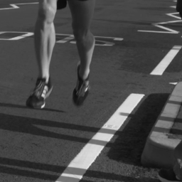
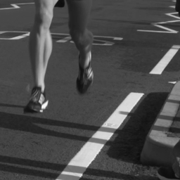
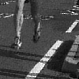
We assume that the true videos are chosen from the datasets Runner [23] and Kobe [31] with $b=8$ as shown in Figures 5 and 6. The mask in the stack $\{M_{i}(m,n)\}_{i=1}^{b}$ is selected as shifting random binary matrices in which the first mask is simulated by a random binary atrix with elements drawn from a Bernoulli distribution with parameter $0.5$ and the subsequent masks shift one pixel horizontally in order [31]. Let $\texttt{x}^{\dagger}=(\texttt{x}_{1}^{\dagger},\ldots,\texttt{x}_{b}^{\dagger})$ be the true solution and $\texttt{M}=(\texttt{M}_{1},\ldots,\texttt{M}_{b})$ be the forward matrix with $\|\texttt{M}\|^{2}=b$ . The exact snapshot measurements of the datasets Runner and Kobe are given by $\texttt{y}^{\dagger}:=\sum_{i=1}^{b}\texttt{M}_{i}\texttt{x}_{i}^{\dagger}$ as shown in Figure 7. In this application, we need to recover $\texttt{x}^{\dagger}\in\mathbb{R}^{(b\times 256^{2})\times 1}$ from the noisy measurement $\texttt{y}^{\delta}\in\mathbb{R}^{256^{2}\times 1}$ with a relative noise level $\delta_{\text{rel}}=0.01$ . This implies that the linear system (38) is under-determined due to the compression between different frames. Additionally, it is important to note that a significant amount of useful information in each frame of the original videos will be lost since nearly half of the elements in every mask are zero.

To solve this ill-posed video reconstruction problem, we incorporate the piece-wise constancy feature of the video into our proposed method, Algorithm 3. To this end, we take

\displaystyle{\mathcal{R}}(\texttt{x})=\sum_{i=1}^{b}{\mathcal{R}}_{i}(\texttt{x}_{i})\quad\mbox{with }{\mathcal{R}}_{i}(\texttt{x}_{i}):=\frac{1}{2}\|\texttt{x}_{i}\|^{2}+\lambda|\texttt{x}_{i}|_{TV},

(39)

where $\lambda>0$ is a positive constant and $|\texttt{x}_{i}|_{TV}$ denotes the 2-dimensional isotropic total variation of $\texttt{x}_{i}$ for each frame; see [1]. It is clear that ${\mathcal{R}}$ satisfies Assumption 3.1 with $\kappa=1/2$ . In order to implement Algorithm 3, we need to update $\texttt{x}_{k+1,i_{k}}^{\delta}$ from $\xi_{k+1,i_{k}}^{\delta}$ which requires to solving a total variation denoising problem of the form

\texttt{x}_{k+1,i_{k}}^{\delta}=\arg\min_{z}\left\{{\mathcal{R}}_{i_{k}}(z)-\langle\xi_{k+1,i_{k}}^{\delta},z\rangle\right\}=\arg\min_{z}\left\{\lambda|z|_{TV}+\frac{1}{2}\|z-\xi_{k+1,i_{k}}^{\delta}\|^{2}\right\}.

In the experiment, this sub-problem is solved by the iterative clipping algorithm [1]. When executing Algorithm 3, we use $\xi_{0}=0$ and $\gamma=2\kappa\mu/b$ with $\mu=1.99$ and for the datasets Runner and Kobe we use $\lambda=15$ and $30$ respectively. We run the algorithm for $1500$ iteration steps and report the reconstruction results in Figure 8 and 9. The detailed numerical results of the above experiments are recorded in Table 2, including the computational time, the peak signal-to-noise ratio (PSNR), the structural similarity index measure (SSIM) [29], and the relative error. These results demonstarte that, with a TV denoiser in the domain of prime variable, Algorithm 3 can recover a great deal of missing information from the compressed snapshot measurement and thus reconstruct a good approximation of the original video within an acceptable amount of time even if the data is corrupted by noise.

	Time (s)	PSNR (db)	SSIM	relative error
Runner	23.5595	27.8292	0.8012	0.0154
Kobe	23.6561	28.3153	0.8883	0.0216

Table 2. Numerical results of Algorithm 3 with

{\mathcal{R}}

given by (39) for the datasets Runner and Kobe using the noisy snapshot measurement with the relative noise level

\delta_{\text{rel}}=0.01

Considering the same problem for Runner and Kobe using the noisy data with $\delta_{\text{rel}}=0.01$ , we run the Algorithm 4 with $\tau=2$ , $\mu=1.99$ , and ${\mathcal{R}}$ given by (39).We use $\lambda=15$ for the datasets Runner and $\lambda=30$ for the dataset Kobe. This algorithm terminates the iteration based on the a posteriori discrepancy principle. The reconstruction results are shown in Figures 10 and 11. We also record the stopping index $k_{\delta}$ , PSNR, SSIM, and relative error of the reconstructions in Table 3. It can be observed that Algorithm 4 consistently terminates the iterations within a finite number of steps and provides efficient reconstructions of the true videos, even when the data is corrupted by noise. Therefore, Algorithm 4 effectively meets the key requirement of automatic stopping for this large-scale video reconstruction in practice.

	$k_{\delta}$	PSNR (db)	SSIM	relative error
Runner	1306	27.5785	0.7983	0.0163
Kobe	2611	28.4458	0.8842	0.0209

Table 3. Numerical results of Algorithm 4 with

{\mathcal{R}}

gicen by (39) for the datasets Runner and Kobe using the noisy snapshot measurement with the relative noise level

\delta_{\text{rel}}=0.01

5. Conclusions

In this paper, we addressed linear ill-posed inverse problems of the separable form $\sum_{i=1}^{b}A_{i}x_{i}=y$ in Hilbert spaces and proposed a randomized block coordinate descent (RBCD) method for solving such problems. Although the RBCD method has been extensively studied for well-posed convex optimization problems, there has been a lack of convergence analysis for ill-posed problems. In this work, we investigated the convergence properties of the RBCD method with noisy data under both a priori and a posteriori stopping rules. We proved that the RBCD method, when combined with an a priori stopping rule, serves as a convergent regularization method in the sense of weak convergence almost surely. Additionally, we explored the early stopping of the RBCD method, demonstrating that the discrepancy principle can terminate the iteration after a finite number of steps almost surely. Furthermore, we developed a strategy to incorporate convex regularization terms into the RBCD method to enhance the detection of solution features. To validate the performance of our proposed method, we conducted numerical simulations, demonstrating its effectiveness.

It should be noted that when the sought solution is smooth and decomposed into many small blocks artificially, the numerical results obtained by the RBCD method, which are not reported here, may not meet expectations due to the mismatch between adjacent blocks. Therefore, there is significant interest in developing novel strategies to overcome this mismatch between adjacent blocks, thereby improving the performance of the RBCD method. However, in cases where the object to be reconstructed naturally consists of many separate frames, such as the coded aperture compressive temporal imaging, the RBCD method demonstrates its effectiveness and yields satisfactory results.

Acknowledgement

The work of Q. Jin is partially supported by the Future Fellowship of the Australian Research Council (FT170100231). The work of D. Liu is supported by the China Scholarship Council program (Project ID: 202307090070).

References

[1] A. Beck and M. Teboulle, Fast gradient-based algorithms for constrained total variation image denoising and deblurring problems, IEEE Trans. Image Process., 18 (2009), pp.2419–2434.
[2] D. P. Bertsekas, Incremental proximal methods for large scale convex optimization, Math. Program., 129 (2011), pp. 163–195.
[3] L. Borg, J. Frikel, J. S. Jørgensen and E. T. Quinto, Analyzing reconstruction artifacts from arbitrary incomplete X-ray CT data, SIAM J. Imaging Sci., 11 (2018), pp. 2786–2814.
[4] P. Brémaud, Probability theory and stochastic processes, Universitext, Springer, Cham, 2020.
[5] P. L. Combettes and J.-C. Pesquet, Stochastic quasi-Fejér block-coordinate fixed point iterations with random sweeping, SIAM J. Optim., 25 (2015), pp. 1221–1248.
[6] H. W. Engl, M. Hanke and A. Neubauer, Regularization of Inverse Problems, Dordrecht, Kluwer, 1996.
[7] J. Frikel and E. T. Quinto, Characterization and reduction of artifacts in limited angle tomography, Inverse Problems, 29 (2013), 125007.
[8] M. Haltmeier, A. Leitão and O. Scherzer, Kaczmarz methods for regularizing nonlinear ill-posedequations. I. Convergence analysis, Inverse Probl. Imaging, 1 (2007), pp. 289–298.
[9] P. C. Hansen and M. Saxild-Hansen, AIR tools—a MATLAB package of algebraic iterative reconstruction methods, J. Comput. Appl. Math., 236 (2012), pp. 2167–2178.
[10] Q. Jin, Landweber-Kaczmarz method in Banach spaces with inexact inner solvers, Inverse Problems, 32 (2016), 104005.
[11] Q. Jin, X. Lu and L. Zhang, Stochastic mirror descent method for linear ill-posed in Banach spaces, Inverse Problems, 39 (2023), 065010.
[12] Q. Jin and W. Wang, Landweber iteration of Kaczmarz type with general non-smooth convex penalty functionals, Inverse Problems, 29 (2013), no. 8, 085011, 22 pp.
[13] R. Kowar and O. Scherzer, Convergence analysis of a Landweber-Kaczmarz method for solving nonlinear ill-posed problems, Ill-posed and inverse problems, 253–270, VSP, Zeist, 2002.
[14] C. Liu, J. Qiu, and M. Jiang, Light field reconstruction from projection modeling of focal stack, Opt. Express, 25 (2017), pp. 11377–11388.
[15] P. Llull, X. Liao, X. Yuan, J. Yang, D. Kittle, L. Carin, G. Sapiro, and D. J. Brady, Coded aperture compressive temporal imaging, Opt. Express, 21 (2013), pp. 10526–10545.
[16] A. K. Louis, Incomplete data problems in X-ray computerized tomography. I. singular value decomposition of the limited angle transform, Numer. Math., 48 (1986), pp. 251–262.
[17] Z. Lu and L. Xiao, On the complexity analysis of randomized block-coordinate descent methods, Math. Program., 152 (2015), 615–642.
[18] F. Natterer, The Mathematics of Computerized Tomography, SIAM, Philadelphia, 2001.
[19] Y. Nesterov, Efficiency of coordinate descent methods on huge-scale optimization problems, SIAM J. Optim., 22 (2012), no. 2, pp. 341–362.
[20] E. T. Quinto, Singularities of the X-ray transform and limited data tomography in $\mathbb{R}^{2}$ and $\mathbb{R}^{3}$ , SIAM J. Appl. Math., 24 (1993), pp. 1215–1225.
[21] S. Rabanser, L. Neumann and M. Haltmeier, Analysis of the block coordinate descent method for linear ill-posed problems, SIAM J. Imaging Sci., 12 (2019), no. 4, pp. 1808–1832.
[22] P. Richtárik and M. Takác, Iteration complexity of randomized block-coordinate descent methods for minimizing a composite function, Math. Program., 144 (2014), 1–38.
[23] Runner data, https://www.videvo.net/video/elite-runner-slow-motion/4541/.
[24] A. Saha and A. Tewari, On the nonasymptotic convergence of cyclic coordinate descent methods, SIAM J. Optim., 23 (2013), pp. 576–601.
[25] P. Tseng, Convergence of a block coordinate descent method for nondifferentiable minimization, J. Optim. Theory Appl., 109 (2001), 475–494.
[26] P. Tseng and S. Yun, Block-coordinate gradient descent method for linearly constrained nonsmooth separable optimization, J. Optim. Theory Appl. 140 (2009), 513–535.
[27] P. Tseng and S. Yun, A coordinate gradient descent method for nonsmooth separable minimization, Math. Program., 117 (2009), 387–423.
[28] A. Wagadarikar, R. John, R. Willett and D. J. Brady, Single disperser design for coded aperture snapshot spectral imaging, Appl. Opt., 47 (2008), pp. B44–B51.
[29] Z. Wang, A. C. Bovik, H. R. Sheikh and E. P. Simoncelli, Image quality assessment: from error visibility to structural similarity, IEEE Trans. Image Process., 13 (2004), pp. 600–612.
[30] S. J. Wright, Coordinate descent algorithms, Math. Program., 151 (2015), pp. 3–34.
[31] J. Yang, X. Yuan, X. Liao, P. Llull, G. Sapiro, D. J. Brady and L. Carin, Video compressive sensing using Gaussian mixture models, IEEE Trans. Image Process., 23 (2014), pp. 4863–4878.
[32] X. Yin, G. Wang, W. Li and Q. Liao, Iteratively reconstructing 4D light fields from focal stacks, Appl. Opt., 55 (2016), pp. 8457–8463.
[33] X. Yuan, D. J. Brady and A. K. Katsaggelos, Snapshot compressive imaging: theory, algorithms, and applications, IEEE Signal Process. Mag., 38 (2021), pp.65–88.
[34] C. Zălinscu, Convex Analysis in General Vector Spaces, World Scientific Publishing Co., Inc., River Edge, New Jersey, 2002.

	$\displaystyle\\|u_{k+1}^{\delta}\\|^{2}$	$\displaystyle=\sum_{i\neq i_{k}}\\|u_{k+1,i}^{\delta}\\|^{2}+\\|u_{k+1,i_{k}}^{\delta}\\|^{2}$
		$\displaystyle=\sum_{i\neq i_{k}}\\|u_{k,i}^{\delta}\\|^{2}+\\|u_{k,i_{k}}^{\delta}-\gamma A_{i_{k}}^{*}(Au_{k}^{\delta}-y^{\delta}+y)\\|^{2}$
		$\displaystyle=\sum_{i\neq i_{k}}\\|u_{k,i}^{\delta}\\|^{2}+\\|u_{k,i_{k}}^{\delta}\\|^{2}+\gamma^{2}\\|A_{i_{k}}^{*}(Au_{k}^{\delta}-y^{\delta}+y)\\|^{2}$
		$\displaystyle\quad\,-2\gamma\langle u_{k,i_{k}}^{\delta},A_{i_{k}}^{*}(Au_{k}^{\delta}-y^{\delta}+y)\rangle$
		$\displaystyle=\\|u_{k}^{\delta}\\|^{2}+\gamma^{2}\\|A_{i_{k}}^{*}(Au_{k}^{\delta}-y^{\delta}+y)\\|^{2}$
		$\displaystyle\quad\,-2\gamma\langle A_{i_{k}}u_{k,i_{k}}^{\delta},Au_{k}^{\delta}-y^{\delta}+y\rangle.$

	$\displaystyle\mathbb{E}[\\|u_{k+1}^{\delta}\\|^{2}\|{\mathcal{F}}_{k}]$
	$\displaystyle=\\|u_{k}^{\delta}\\|^{2}+\frac{\gamma^{2}}{b}\sum_{i=1}^{b}\\|A_{i}^{*}(Au_{k}^{\delta}-y^{\delta}+y)\\|^{2}-\frac{2\gamma}{b}\left\langle\sum_{i=1}^{b}A_{i}u_{k,i}^{\delta},Au_{k}^{\delta}-y^{\delta}+y\right\rangle$
	$\displaystyle=\\|u_{k}^{\delta}\\|^{2}+\frac{\gamma^{2}}{b}\\|A^{*}(Au_{k}^{\delta}-y^{\delta}+y)\\|^{2}-\frac{2\gamma}{b}\left\langle Au_{k}^{\delta},Au_{k}^{\delta}-y^{\delta}+y\right\rangle$
	$\displaystyle\leq\\|u_{k}^{\delta}\\|^{2}+\frac{\gamma^{2}\\|A\\|^{2}}{b}\\|Au_{k}^{\delta}-y^{\delta}+y\\|^{2}-\frac{2\gamma}{b}\\|Au_{k}^{\delta}-y^{\delta}+y\\|^{2}$
	$\displaystyle\quad\,-\frac{2\gamma}{b}\langle y^{\delta}-y,Au_{k}^{\delta}-y^{\delta}+y\rangle$
	$\displaystyle\leq\\|u_{k}^{\delta}\\|^{2}-\frac{1}{b}(2-\gamma\\|A\\|^{2})\gamma\\|Au_{k}^{\delta}-y^{\delta}+y\\|^{2}+\frac{2\gamma}{b}\delta\\|Au_{k}^{\delta}-y^{\delta}+y\\|.$

	$\displaystyle\\|x_{k+1}-\bar{x}\\|^{2}$	$\displaystyle=\sum_{i\neq i_{k}}\\|x_{k+1,i}-\bar{x}_{i}\\|^{2}+\\|x_{k+1,i_{k}}-\bar{x}_{i_{k}}\\|^{2}$
		$\displaystyle=\sum_{i\neq i_{k}}\\|x_{k,i}-\bar{x}_{i}\\|^{2}+\\|x_{k,i_{k}}-\bar{x}_{i_{k}}-\gamma A_{i_{k}}^{*}(Ax_{k}-y)\\|^{2}$
		$\displaystyle=\sum_{i\neq i_{k}}\\|x_{k,i}-\bar{x}_{i}\\|^{2}+\\|x_{k,i_{k}}-\bar{x}_{i_{k}}\\|^{2}+\gamma^{2}\\|A_{i_{k}}^{*}(Ax_{k}-y)\\|^{2}$
		$\displaystyle\quad\,-2\gamma\langle x_{k,i_{k}}-\bar{x}_{i_{k}},A_{i_{k}}^{*}(Ax_{k}-y)\rangle$
		$\displaystyle=\\|x_{k}-\bar{x}\\|^{2}+\gamma^{2}\\|A_{i_{k}}^{*}(Ax_{k}-y)\\|^{2}$
		$\displaystyle\quad\,-2\gamma\langle A_{i_{k}}(x_{k,i_{k}}-\bar{x}_{i_{k}}),Ax_{k}-y\rangle.$

	$\displaystyle\mathbb{E}[\\|x_{k+1}-\bar{x}\\|^{2}\|{\mathcal{F}}_{k}]$
	$\displaystyle=\\|x_{k}-\bar{x}\\|^{2}+\frac{\gamma^{2}}{b}\sum_{i=1}^{b}\\|A_{i}^{*}(Ax_{k}-y)\\|^{2}-\frac{2\gamma}{b}\sum_{i=1}^{b}\langle A_{i}(x_{k,i}-\bar{x}_{i}),Ax_{k}-y\rangle$
	$\displaystyle=\\|x_{k}-\bar{x}\\|^{2}+\frac{\gamma^{2}}{b}\\|A^{*}(Ax_{k}-y)\\|^{2}-\frac{2\gamma}{b}\langle A(x_{k}-\bar{x}),Ax_{k}-y\rangle$
	$\displaystyle\leq\\|x_{k}-\bar{x}\\|^{2}+\frac{\gamma^{2}\\|A\\|^{2}}{b}\\|Ax_{k}-y\\|^{2}-\frac{2\gamma}{b}\\|Ax_{k}-y\\|^{2}$

	$\displaystyle-\\|z_{l}-\tilde{z}\\|$	$\displaystyle\leq\liminf_{k\to\infty}\left\{\\|x_{k}(\omega)-\tilde{z}\\|-\\|x_{k}(\omega)-z_{l}\\|\right\}$
		$\displaystyle\leq\limsup_{k\to\infty}\left\{\\|x_{k}(\omega)-\tilde{z}\\|-\\|x_{k}(\omega)-z_{l}\\|\right\}$
		$\displaystyle\leq\\|z_{l}-\tilde{z}\\|.$