Randomised Gaussian Process Upper Confidence Bound for Bayesian Optimisation
Abstract
In order to improve the performance of Bayesian optimisation, we develop a modified Gaussian process upper confidence bound (GP-UCB) acquisition function. This is done by sampling the exploration-exploitation trade-off parameter from a distribution. We prove that this allows the expected trade-off parameter to be altered to better suit the problem without compromising a bound on the function’s Bayesian regret. We also provide results showing that our method achieves better performance than GP-UCB in a range of real-world and synthetic problems.
1 Introduction
Global optimisation is a cornerstone of modern scientific innovation. Optimisation of alloys and other materials has allowed us to create massive vehicles that are both strong and light enough to fly. Optimisation in medical science has seen us live longer and healthier lives than previously thought possible. This optimisation usually involves a trial-and-error approach of repeated experiments with different inputs to determine which input produces the most desirable output. Unfortunately, many system are expensive to sample, and the heuristic methods commonly used to select inputs are not sample-efficient. This can lead to these optimisation experiments being prohibitively costly. As such, methods that can select inputs in a sample-efficient manner can lead to faster and cheaper innovation in a wide range of fields.
Bayesian optimisation is one of the most sample efficient methods for optimising expensive, noisy systems. It has shown excellent performance on a range of practical problems, including problems in biomedical science Turgeon et al. (2016); Gonzalez et al. (2015), materials science Li et al. (2017); Ju et al. (2017), and machine learning Snoek et al. (2012); Klein et al. (2017); Xia et al. (2017). It does so by using the data from previous samples to generate a statistical model of the system. This model is then used to suggest the next input through an acquisition function. The design of the acquisition function is non-trivial; and is critically important to the algorithms performance. It must balance selecting points with the goal of improving the statistical model (exploration), and selecting points with the goal of utilising the improved statistical model to find the global optima (exploitation). In addition to this, the costly nature of these problems means that it is desirable to have a theoretical guarantee of the algorithm’s performance.
There are a large range of acquisition functions, all with different balances of exploration and exploitation, but we focus on Gaussian process upper confidence bound (GP-UCB) Srinivas et al. (2010) in this work. This controls its exploration-exploitation trade-off with a single hyperparameter, . It has strong theoretical guarantees on the overall convergence rate, but the bound they give is fairly loose. This causes the value of to be too large, causing significant over-exploration and hence poor practical performance. In practice, the theoretical guarantees need to be weakened by selecting a far smaller .
We introduce a novel modification to the GP-UCB acquisition function that significantly improves its exploration-exploitation balance while still having a strong convergence guarantee. This is done by sampling its trade-off parameter with a distribution that allows for a range of exploration factors. However, the distribution is chosen such that convergence is guaranteed to be sub-linear while the sampled is generally smaller than the traditional GP-UCB. This reduction leads to a direct improvement on the convergence efficiency in practice. We demonstrate this improved performance over the standard GP-UCB implementation in a range of both synthetic benchmark functions and real-world applications.
In summary, our contributions are:
-
•
The development of a modified acquisition function: RGP-UCB.
-
•
A convergence analysis of Bayesian optimisation using RGP-UCB.
-
•
The demonstration of the performance of our method on a range of synthetic and real-world problems.
2 Background
In this section, we provide a brief overview of Bayesian optimisation, with an emphasis on acquisition functions and regret bounds. For a more in-depth overview of Bayesian optimisation, we refer readers to Rasmussen and Williams (2006) and Brochu et al. (2010).
2.1 Bayesian Optimisation
Bayesian optimisation is a method for optimising expensive, noisy black-box functions. It represents the system being optimised as an unknown function, . As this is black-box, it is impossible to directly observe. However, we can sample it with an input variable, , to obtain a noisy output, , where is the random noise corrupting the measurement. Bayesian optimisation seeks to efficiently find the optimal input for such systems over a bounded search space, :
| (1) |
To do this, it creates a statistical model of using all previously sampled input-output pairs, . This statistical model is usually a Gaussian process, but other models can be used. The statistical model is then used to create an acquisition function, . This is essentially a map of our belief of how useful a given input will be for optimising the system. As such, it can be used to suggest ; the next input with which to sample the system. This input and its corresponding output can then be added to the previous data, . This process can be iterated, with the Gaussian process improving with each iteration, until a stopping condition has been met. As Bayesian optimisation is generally used on expensive systems, this stopping condition is often a maximum number of experiments, .
2.2 Gaussian Process
The Gaussian process is the most common statistical model used in Bayesian optimisation. It models each point in as a Gaussian random variable. As such, it is completely characterised by a mean function, , and a variance function, . However, in order to model sensibly behaved functions there must be correlation between neighbouring points. This is done by conditioning the distribution on the data via a kernel function. There are many viable kernel functions, but one of the simplest and most popular is the squared exponential kernel as it only depends on a single hyperparameter, the lengthscale . This is given by
| (2) |
Using a kernel such as this, a predictive distribution, , can be obtained by conditioning the Gaussian process on the data, :
| (3) | |||||
where is the kernel matrix, , and . Here is the identity matrix with the same dimensions as , and is the output noise standard deviation.
2.3 Acquisition Functions
Once the Gaussian process has been generated, it must then be used to create an acquisition function. This is chosen such that its global maxima in will be the best next point to sample:
| (4) |
However, the design of such a function is non-trivial. It must first suggest points spread over the search space to improve the Gaussian process. This is called exploration. Once the Gaussian process has been improved enough, it must then transition to suggesting points in regions that have a high probability of containing the global optima. This is called exploitation. If an acquisition function does not explore enough, it may get stuck exploiting sub-optimal regions and never find the global optima. However, if it explores too much, it may waste costly evaluations improving an already adequate Gaussian process. This makes balancing exploration and exploitation vital. There is a wide range of common acquisition functions, all of which have different balances of exploration and exploitation. These include entropy search (ES) by Hennig and Schuler (2012), predictive entropy search (PES) by Hernández-Lobato et al. (2014), knowledge gradient (KG) by Scott et al. (2011), and others. However, we will only consider the Gaussian process upper confidence bound (GP-UCB) by Srinivas et al. (2010), Thompson sampling by Russo and Van Roy (2014), and expected improvement (EI) by Jones et al. (1998), with the latter two only being used as baselines.
2.3.1 GP-UCB
GP-UCB Srinivas et al. (2010) is one of the most intuitive acquisition functions. It balances exploration and exploitation through a single hyperparameter, :
| (5) |
Increasing makes the acquisition function favour points with high variance, causing more exploration. Decreasing will make the acquisition function favour points with high mean, causing more exploitation. However, the selection of is not done to optimally balance exploitation and exploration, but is done such that the cumulative regret is bounded. It has been proved that, assuming the chosen kernel satisfies
| (6) |
for some constants , then with probability , the algorithm will have sub-linear regret if
| (7) |
While the regret bound provided by this choice of is desirable, it unfortunately is far larger than needed. This leads to sub-optimal real world performance due to over-exploration. In their own paper, the authors divided the suggested by a factor of 5 to achieve better performance Srinivas et al. (2010).
3 Proposed Method
In this section we describe our improved GP-UCB acquisition function, randomised Gaussian process upper confidence bound (RGP-UCB), and prove that it has a sub-linear regret bound.
3.1 RGP-UCB
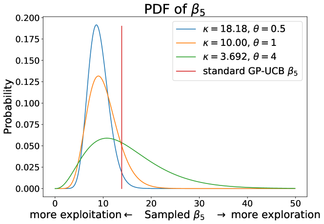
While the standard GP-UCB method has a desirable regret bound, it has relatively poor performance. This is due to the used to satisfy this bound being far too large, forcing significant over-exploration. As such, a method for selecting a smaller while maintaining a regret bound is desirable. We show that this can be done by sampling from a distribution, and as such, we call our method randomised Gaussian process upper confidence bound (RGP-UCB). Doing so means that we bound the Bayesian regret instead of the regret, but it allows for far greater freedom in selecting , letting it be set far smaller while still maintaining convergence guarantees. However, we require since a negative will punish exploration. We also do not want our distribution to suggest a very large as that will cause over-exploration. As such, we draw from a distribution. Examples of this distribution can be seen in Figure 1 and the complete algorithm is shown in Algorithm 1. Much like with standard GP-UCB, the parameters of this distribution are chosen to satisfy a regret bound, as per Theorem 3. However, we show that we only need to set one of the two distribution parameters for the bound to hold. Unlike the standard GP-UCB, this allows us to tune to substantially improve our methods performance without compromising its theoretical guarantees.
Input:, scale parameter, , # Iterations , Kernel lengthscale
3.2 Theoretical Analysis
Bayesian optimisation is commonly used in high value problems. As such, theoretical measures of its convergence are desirable. The cumulative regret is one such measure, and is the cornerstone of GP-UCB Srinivas et al. (2010). Regret is simply the difference between the current sampled value and the global optima. The cumulative regret is the sum of the regret over all iterations:
| (8) |
As RGP-UCB is probabilistic, we instead need to use the Bayesain regret by Russo et al Russo and Van Roy (2014):
| (9) |
However, their proof was for Gaussian processes with a finite search space, i.e. . As such, we follow a method similar to Srinivas et al. (2010) and Kandasamy et al. (2017) and introduce a discretisation of our search space into an grid of equally spaced points, . We denote as the closest point to in .
With this, we can begin bounding the Bayesian regret of our algorithm by decomposing it into components that are easier to bound.
Lemma 1.
The Bayesian regret of a probabilistic RGP-UCB algorithm, , over iterations can be decomposed as
| (10) | |||||
Proof.
This simply follows from the fact that, as , we have that . ∎
With this decomposition, we simply need to find a bound for each term to bound the Bayesian regret. We will start with the second term.
Theorem 1.
Assuming that is drawn from a distribution with , the following bound holds
| (11) | |||||
Proof.
As the posterior distribution of at iteration is , the distribution of , is simply ,). Hence
| (12) | |||||
We note that the exponential term is simply the moment generating function of , which has a closed form for a gamma distribution. This lets us express our inequality as
| (13) | |||||
As we want this to decay at a sub-linear rate, we need
| (14) |
Setting to satisfy this, equation is bounded by the following:
| (15) | |||||
∎
Next, we attempt to bound the first component.
Theorem 2.
Assuming that is drawn from a distribution, the following bound holds
| (16) | |||||
Proof.
Using Jensen’s Inequality we have
| (17) | |||||
We can then use the Cauchy-Schwartz inequality to get
| (18) | |||||
As is a gamma distribution with shape parameter and scale parameter , its maximum is given by
| (19) |
where is the Euler-Mascheroni constant and is the inverse CDF of . This finally gives us the following bound:
| (20) | |||||
∎
Finally, we need to bound components and . For these, we can use lemma 10 from Kandasamy et al. (2017).
Lemma 2.
At step , for all , .
This means that we have that
| (21) | |||||
With this we can finally find our Bayesian regret bound.
Theorem 3.
If is sampled from a distribution with
| (22) |
then the RGP-UCB acquisition function has its Bayesian regret bounded by
| (23) | |||||
where is the Euler-Mascheroni constant and is the inverse CDF of
Proof.
The result follows simply by combining the bounds for the various components. ∎
4 Results
In this section we present results that demonstrate the performance of RGP-UCB in comparison to other common acquisition functions. We also demonstrate the impact of varying the parameter of the gamma distribution used to sample . The Python code used for this paper can be found at https://github.com/jmaberk/RGPUCB.
4.1 Experimental Setup
We test our method against a selection of common acquisition functions on a range of Bayesian optimisations problems. These include a range of synthetic benchmark functions and real-world optimisation problems. In each case, the experiment was run for iterations and repeated 10 times with different initial points. The initial points are chosen randomly with a Latin hypercube sample scheme Jones (2001). The methods being tested are:
-
•
Our randomised Gaussian process upper confidence bound with (RGP-UCB ).
-
•
Our randomised Gaussian process upper confidence bound with (RGP-UCB ).
-
•
Our randomised Gaussian process upper confidence bound with (RGP-UCB ).
-
•
Standard Gaussian process upper confidence bound (GP-UCB) Srinivas et al. (2010).
-
•
Expected improvement (EI) Jones et al. (1998).
-
•
Thompson sampling (Thompson) Russo and Van Roy (2014).
Note that we turn all functions that are traditionally minimised into maximisation problems by taking their negative for consistency. As such, higher results are always better.
4.2 Selection of the Trade-off Parameter
An advantage of our method is that it can change its exploration-exploitation balance without compromising its convergence guarantee. This is done by changing the parameter in the distribution. Increasing will increase the expected , increasing exploration.
As different problems favour different exploration-exploration balances, we tested a range of values on a range of different problems. In Figure 2, we show the performance of a range of values on an exploitation favouring problem, the Alpine 2 (5D) function, and an exploration favouring problem, the Dropwave (2D) function.
| Dropwave (2D) | Alpine 2 (5D) | |
|---|---|---|
| 0.738 6.7e-2 | 78.912.4 | |
| 0.755 5.0e-2 | 92.112.2 | |
| 0.754 6.9e-2 | 77.812.7 | |
| 0.727 8.6e-2 | 77.512.5 | |
| 0.847 5.7e-2 | 71.513.6 | |
| 0.848 3.3e-2 | 43.49.84 | |
| 0.814 6.2e-2 | 45.410.0 |
It was found that gives good performance on both the above exploration-favouring problem and other similar problems tested. Likewise, is a good choice for exploitation favouring problems. We also note that has decent performance on both problems, making it a good choice for problems where the required exploration-exploitation balance is completely unknown.
4.3 Synthetic Benchmark Functions
The first demonstration of our methods performance is the optimisation of several common synthetic benchmark functions. These are the Dropwave (2D), Sphere (4D), Alpine 2 (5D), and Ackley (5D) functions222All benchmark functions use the recommended parameters from https://www.sfu.ca/~ssurjano/optimization.html. Results for these are shown in Figure 3.


Here we can see that RGP-UCB has competitive performance in all of the above cases. In general, it does significantly better than the standard GP-UCB and the Thompson sampling acquisition functions. EI has better early performance in many cases, as it starts exploiting earlier. However, RGP-UCB tends to have better exploration and therefore often able to beat it in the long-term.
The leftmost functions were chosen to be pathological cases which disproportionately favours exploration (Dropwave 2D) and exploitation (Sphere 4D). These can be seen as best-case examples for GP-UCB and EI respectively. However, RGP-UCB is able to out-perform them even on these if its parameter is chosen properly, and does so while maintaining its convergence guarantee. This formulation of EI does not have a known regret bound as it follows the standard implementation and hence doesn’t satisfy the assumptions required by the current bounds Bull (2011); Ryzhov (2016); Wang and de Freitas (2014); Nguyen et al. (2017).
In the middle two plots, RGP-UCB is superior even with the conservative parametrisation of .
4.4 Machine Learning Hyperparameter Tuning
Our first demonstration of the real-world performance of RGP-UCB is the hyperparameter tuning of a support vector regression (SVR) Drucker et al. (1997) algorithm. This is the support vector machine classification algorithm extended to work on regression problems, with performance measured in root mean squared error (RMSE). It has three hyperparameters, the threshold, , the kernel parameter, , and a soft margin parameter, . All experiments are done with the public Space GA scale dataset 333 Dataset can be found at https://www.csie.ntu.edu.tw~cjlin/libsvmtools/datasets/regression.html. The results are shown in Figure 3.
We can see that the final performance of all three variants of our method exceeds that of standard GP-UCB. The high exploitation and balanced variants are competitive with EI, with the former achieving higher final performance. As with many real-world problems, SVR is known to favour higher exploitation, and is therefore an example of when the user would know to try a smaller .
4.5 Materials Science Application: Alloy Heat Treatment
The second demonstration of RGP-UCB’s performance is the optimisation of a Aluminium-Scandium alloy heat treatment simulation Robson et al. (2003). The goal of the simulation is to optimise the resulting alloys hardness, measured in MPa. The hardening process is controlled through multiple cooking stages, each with two hyperparametrs, the duration and a temperature. As we use a two-stage cooking simulation, there is a total of four hyperparameters to optimise through Bayesian optimisation. The results are shown in Figure 3.
The results are very similar to the previous SVR example, with the high-exploitation method having the best performance and the balance method being competitive with EI.
4.6 Conclusion
We have developed a modified UCB based acquisition function that has substantially improved performance while maintaining a sub-linear regret bound. We have proved that this bound holds in terms of Bayesian regret while allowing for some flexibility in the selection of its parameters. We have also demonstrated the impact of said parameters on the performance. Moreover, we have shown that its performance is competitive or greater than existing methods in a range of synthetic and real-world applications.
Acknowledgements
This research was supported by an Australian Government Research Training Program (RTP) Scholarship awarded to JMA Berk, and was partially funded by the Australian Government through the Australian Research Council (ARC). Prof Venkatesh is the recipient of an ARC Australian Laureate Fellowship (FL170100006).
References
- Brochu et al. [2010] Eric Brochu, Vlad M Cora, and Nando De Freitas. A tutorial on bayesian optimization of expensive cost functions, with application to active user modeling and hierarchical reinforcement learning. arXiv preprint arXiv:1012.2599, 2010.
- Bull [2011] Adam D Bull. Convergence rates of efficient global optimization algorithms. Journal of Machine Learning Research, 12(Oct):2879–2904, 2011.
- Drucker et al. [1997] Harris Drucker, Christopher JC Burges, Linda Kaufman, Alex J Smola, and Vladimir Vapnik. Support vector regression machines. In Advances in neural information processing systems, pages 155–161, 1997.
- Gonzalez et al. [2015] Javier Gonzalez, Joseph Longworth, David C James, and Neil D Lawrence. Bayesian optimization for synthetic gene design. arXiv preprint arXiv:1505.01627, 2015.
- Hennig and Schuler [2012] Philipp Hennig and Christian J Schuler. Entropy search for information-efficient global optimization. Journal of Machine Learning Research, 13(Jun):1809–1837, 2012.
- Hernández-Lobato et al. [2014] José Miguel Hernández-Lobato, Matthew W Hoffman, and Zoubin Ghahramani. Predictive entropy search for efficient global optimization of black-box functions. In Advances in neural information processing systems, pages 918–926, 2014.
- Jones et al. [1998] Donald R Jones, Matthias Schonlau, and William J Welch. Efficient global optimization of expensive black-box functions. Journal of Global optimization, 13(4):455–492, 1998.
- Jones [2001] D. R Jones. A taxonomy of global optimization methods based on response surfaces. Journal of global optimization, 21(4):345–383, 2001.
- Ju et al. [2017] Shenghong Ju, Takuma Shiga, Lei Feng, Zhufeng Hou, Koji Tsuda, and Junichiro Shiomi. Designing nanostructures for phonon transport via bayesian optimization. Physical Review X, 7(2):021024, 2017.
- Kandasamy et al. [2017] Kirthevasan Kandasamy, Akshay Krishnamurthy, Jeff Schneider, and Barnabás Póczos. Asynchronous parallel bayesian optimisation via thompson sampling. arXiv preprint arXiv:1705.09236, 2017.
- Klein et al. [2017] Aaron Klein, Stefan Falkner, Simon Bartels, Philipp Hennig, and Frank Hutter. Fast bayesian optimization of machine learning hyperparameters on large datasets. In International Conference on Artificial Intelligence and Statistics (AISTATS 2017), pages 528–536. PMLR, 2017.
- Li et al. [2017] Cheng Li, David Rubín de Celis Leal, Santu Rana, Sunil Gupta, Alessandra Sutti, Stewart Greenhill, Teo Slezak, Murray Height, and Svetha Venkatesh. Rapid bayesian optimisation for synthesis of short polymer fiber materials. Scientific reports, 7(1):1–10, 2017.
- Nguyen et al. [2017] Vu Nguyen, Sunil Gupta, Santu Rana, Cheng Li, and Svetha Venkatesh. Regret for expected improvement over the best-observed value and stopping condition. In Asian Conference on Machine Learning, pages 279–294, 2017.
- Rasmussen and Williams [2006] Carl Edward Rasmussen and Christopher KI Williams. Gaussian Processes for Machine Learning. MIT Press, 2006.
- Robson et al. [2003] JD Robson, MJ Jones, and PB Prangnell. Extension of the n-model to predict competing homogeneous and heterogeneous precipitation in al-sc alloys. Acta Materialia, 51(5):1453–1468, 2003.
- Russo and Van Roy [2014] Daniel Russo and Benjamin Van Roy. Learning to optimize via posterior sampling. Mathematics of Operations Research, 39(4):1221–1243, 2014.
- Ryzhov [2016] Ilya O Ryzhov. On the convergence rates of expected improvement methods. Operations Research, 64(6):1515–1528, 2016.
- Scott et al. [2011] Warren Scott, Peter Frazier, and Warren Powell. The correlated knowledge gradient for simulation optimization of continuous parameters using gaussian process regression. SIAM Journal on Optimization, 21(3):996–1026, 2011.
- Snoek et al. [2012] Jasper Snoek, Hugo Larochelle, and Ryan P Adams. Practical bayesian optimization of machine learning algorithms. In Advances in neural information processing systems, pages 2951–2959, 2012.
- Srinivas et al. [2010] Niranjan Srinivas, Andreas Krause, Sham M Kakade, and Matthias Seeger. Gaussian process optimization in the bandit setting: no regret and experimental design. In Proceedings of the 27th International Conference on Machine Learning, pages 1015–1022, 2010.
- Turgeon et al. [2016] Martine Turgeon, Cindy Lustig, and Warren H Meck. Cognitive aging and time perception: roles of bayesian optimization and degeneracy. Frontiers in aging neuroscience, 8:102, 2016.
- Wang and de Freitas [2014] Ziyu Wang and Nando de Freitas. Theoretical analysis of bayesian optimisation with unknown gaussian process hyper-parameters. NIPS Workshop on Bayesian Optimization, 2014.
- Xia et al. [2017] Yufei Xia, Chuanzhe Liu, YuYing Li, and Nana Liu. A boosted decision tree approach using bayesian hyper-parameter optimization for credit scoring. Expert Systems with Applications, 78:225–241, 2017.